Electrophoresis of Charged Macromolecules

Electrophoresis of Charged Macromolecules

Christian Holm

Institut für Computerphysik, Universität Stuttgart Stuttgart, Germany

Charge stabilized Colloids!

The analytical description of charged colloidal suspensions is problematic:!

n 

Long ranged interactions: electrostatics/

hydrodynamics!

n 

Inhomogeneous/asymmetrical systems!

n 

Many-body interactions!

!

!

Alternative: the relevant microscopic degrees of freedom are simulated via Molecular Dynamics!

● Explicit particles (ions) with charges

● Implicit solvent approach, but hydrodynamic interactions of the solvent are included via a Lattice-Boltzmann algorithm

ε

Test of LB implementation for Poiseuille!

Simulation box of size 80x40x10.

Velocity profile for a Poiseuille flow in a channel, which is tilted by 45◦ relative to the Lattice-Boltzmann node mesh.

Computed using ESPResSo.

Profile of the absolute fluid velocity of the Poiseuille flow in the 45◦ tilted channel. Red crosses represent simulation data, the blue line is the theoretical result and the dashed blue line represents the theoretical result, using the channel width as a fit

parameter

EOF in a Slit Pore!

4!

Simulation results for a water system. Solid lines denote simulation results, the dotted lines show the analytical results for comparison. Red stands for ion density in particles per nm³, blue stands for the fluid velocity in x-direction, green denotes the particle velocity. All quantities in simulation units.

Colloidal Electrophoresis!

F_E

Electric field E

E Z

F

=

ν

eff eff

µ γ

E v = Observable: mobilty µ =

µ πη

µ

= 6 

Zeff

−

T k e

B ⁴πε length

Bjerrum

2

 =

viscosity η

local force balance F_E = F_Drag leads to stationary state

SEM (O‘Brien, White 1978)!

€

Z ˜ = Zl

/ R

D_i: collective diffusion coefficient

€

κ² = 4π^l_B

∑

€

f_i = c_i / z²_jc _j

i

#

∑

$ % &

' (

Dimensional Analysis

1622 E L E C T R O P H O R E T I C MOBILITY OF A C O L L O I D A L P A R T I C L E

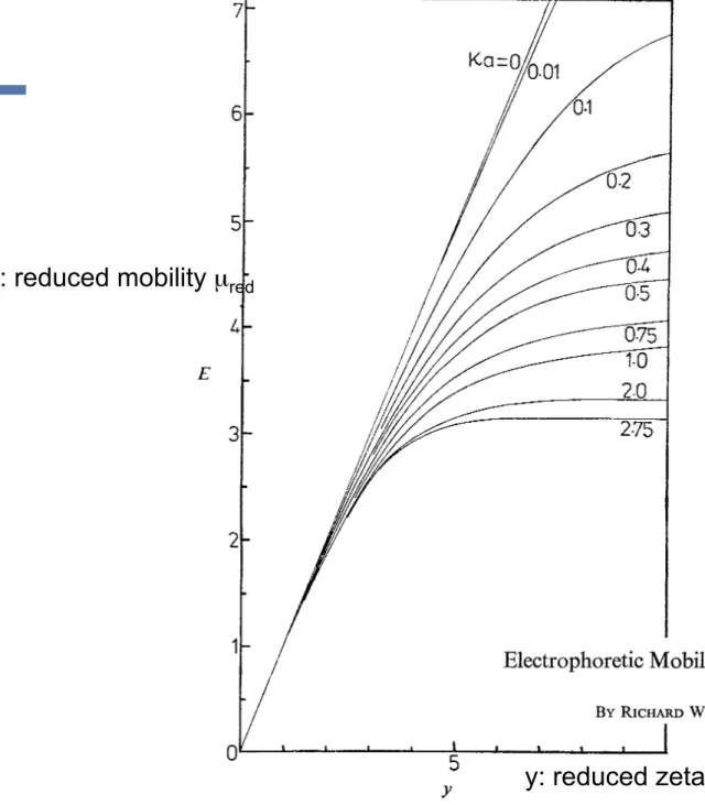
as a function of K a for specific values of the dimensionless zeta potential

(9.2) y = - 4

kT‘

This is not the most convenient way of plotting p ( r , h-a) if the graphs are to be used for converting experimental mobility measurements to zeta potentials, since these experiments are usually carried out at fixed electrolyte concentration, i.e., fixed K a .

I

E

E ”

4

E

3

2

1

0

I I

I , , l l * , ,

5

Y

FIG. 3.-Reduced mobility E of a spherical colloidal particle in a KCl solution as a function of reduced zeta potential y , for ^KU < 2.75. In this regime the mobility appears to increase monotoni-

cally with zeta potential.

We have adopted the alternative procedure for plotting E as a function of y for various

K a values. This has the additional advantage of mimicking the form of a typical experiment where mobility is changed, at fixed ^IC, by systematically varying the concentration of a potential determining ion. This is due to the monotonic variation of surface potential with the p.d.i. concentration. Since the chemist usually has control over the value of Ica, the experiment can be performed with a K a value corres- ponding to a computed curve.

Downloaded by Universitat Stuttgart on 25 March 2011 Published on 01 January 1978 on http://pubs.rsc.org | doi:10.1039/F29787401607

View Online

Electrophoretic Mobility of a Spherical Colloidal Particle

B Y RICHARD w. O’BRIENt AND LEE R. ^WHITEf*

Department of Applied Mathematics, Institute of Advanced Studies, Research School of Physical Sciences, The Australian National University,

Canberra, A.C.T. 2600, Australia Received 13th February, 1978

The equations which govern the ion distributions and velocities, the electrostatic potential and the hydrodynamic flow field around a solid colloidal particle in an applied electric field are re- examined. By using the linearity of the equations which determine the electrophoretic mobility, we show that for a colloidal particle of any shape the mobility is independent of the dielectric properties of the particle and the electrostatic boundary conditions on the particle surface. The mobility depends only on the particle size and shape, the properties of the electrolyte solution in which it is suspended, and the charge inside, or electrostatic potential on, the hydrodynamic shear plane in the absence of an applied field or any macroscopic motion.

New expressions for the forces acting on the particle are derived and a novel substitution is developed which leads to a significant decoupling of the governing equations. These analytic developments allow for the construction of a rapid, robust numerical scheme for the solution of the governing equations which we have applied to the case of a spherical colloidal particle in a general electrolyte solution. We describe a computer program for the conversion of mobility measurements to zeta potential for a spherical colloidal particle which is far more flexible than the Wiersema graphs which have traditionally been used for the interpretation of mobility data. Furthermore it is free of the high zeta potential convergence difficulties which limited Wiersema’s calculations to moderate values of 5. Some sample computations in typical 1 : 1 and 2 : 1 electrolytes are exhibited which illustrate the existence of a maximum in the mobility at high zeta potentials. The physical explanation of this effect is given. The importance of the mobility maximum in testing the validity of the governing equations of electrophoresis and its implications for the colloid chemist’s picture of the Stern layer are briefly discussed.

1. INTRODUCTION

The velocity at which a charged colloidal particle moves in the presence of a weak For a spherical electric field is linearly related to E, the strength of the applied field.

particle this relation takes the form 5

U = pE,

where U is the velocity, and _p is termed the “electrophoretic mobility” of the particle. This paper deals with the problem of calculating the quantity _p.

The electrophoretic velocity U is determined by the balance between the electrical and viscous forces which act on the particle, a balance which is strongly affected by the concentrations of the electrolyte ions in the solvent. In order to understand the way in which the ions affect the forces which act on the particle, we must consider the motion of ions around a spherical particle moving under the action of a steady electric field.

t Rothmans Fellow ; Queen Elizabeth I1 Fellow.

Downloaded by Universitat Stuttgart on 25 March 2011 Published on 01 January 1978 on http://pubs.rsc.org | doi:10.1039/F29787401607

View Online

E: reduced mobility µ_red

y: reduced zeta-potentoial ζ_red

R . w. O ’ B R I E N A N D L . R . W H I T E 1623 The point is academic however since the method, presented in the previous sections of this paper, enables a rapid, exact numerical solution to the general mobility problem.* Thus the chemist, armed with this computer program can generate mobility as a function of zeta potential for the ^{K a} value, the particular electrolyte solution, and temperature of interest to himself. In view of this, the utility of displaying graphs of p(5, K-a) for restricted electrolyte systems, as a conversion aid for the experimentalist, seems marginal.

7 - r

6 -

5-

4 - E

3-

2-

Y

curves have a maximum.

FIG. 4.-Variation of mobility in KCI with zeta potential for KLZ > ^3. In this case the mobility

However, we have solved the mobility equations for a typical 1 : 1 electrolyte, viz. KCl, in order to display some of the striking features of the function &, ^ica).

In fig. 3, we have plotted the reduced mobility E in KCl solution as a function of reduced zeta potential y (on the positive side where Cl- is the counterion) for values of rca 5 2.75. The following important features of fig. 3 should be noted: (i) in

* A copy of the program constructed as a self-contained Fortran subroutine is available from the authors.

Downloaded by Universitat Stuttgart on 25 March 2011 Published on 01 January 1978 on http://pubs.rsc.org | doi:10.1039/F29787401607

View Online

1624 E L E C T R O P H O R E T I C M O B I L I T Y O F A C O L L O I D A L P A R T I C L E

the region where Wiersema could obtain solutions to the equations [i.e., y

<

( ^N 125 mV)] our results are in agreement. (ii) For all rca values 52.75, the mobility is a monotonic increasing function of the zeta potential [at least in the experimentally accessible range y < lO(w-250 mV)]. (iii) At low values of zeta potential, all curves asymptote to the Huckel form

irrespective of ^ica value. (iv) For values of Ka

-

All these features are also present in Wiersema's work but are obscured by his method of displaying

&,

E = y (9.3)

I

I I I * , I

21 ' '

" " " '

ua

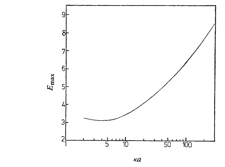
FIG. 5.-Maximum mobility of a spherical particle in KCl as a function of ^ua.

It is this restriction which prevented Wiersema from displaying, in a definitive ^way, the most important feature of the ^p([, rca) function, viz. the maximum in the mobility

as a function of zeta potential for all values of rca

2

2

(ii) the value of the maximum mobility increases with rca for rca > 4 (the very shallow maximum for rca ⁼ 3 is, however, slightly higher than the rca = 4 value); (iii) the reduced zeta potential corresponding to the maximum mobility is

-

-

E = 3y _(9.4)

as rca is increased although, unlike the small ^{K a} curves, there is no regime where all curves reduce to the Smoluchowski form and become independent of K a . In fig. 5, we plot the maximum mobility as a function of rca for KCl electrolyte. The behaviour of the maximum around rca ^N 3 implies that the zeta potential corresponding to the maximum quickly moves to high values as ^{K a} is reduced below -4.

The maximum in the mobility presumably arises from the fact that the electro- phoretic retarding forces which act on a particle increase at a faster rate with

c

does the driving force ; at low values of zeta, this is clearly the case, since the driving

Downloaded by Universitat Stuttgart on 25 March 2011 Published on 01 January 1978 on http://pubs.rsc.org | doi:10.1039/F29787401607

View Online

a=R in lecture notes notation

10!

R . w. O’BRIEN A N D L . R . WHITE 1625 the electrical retarding force due to the distorted charge cloud is proportional to

c2,

for this term involves the product of the particle surface charge density and the field due to the charge cloud, and both these terms are proportional to

[.

The reason that no maximum is observed in the mobility curves for Ica

<

the range y < 10 is probably due to the fact that, for fixed zeta potential the distortion

6p(r) of the double layer and the body force on the fluid vanish as ^KU is decreased to zero. Therefore, although the retarding forces increase more rapidly with

c

the driving force, they will have small magnitude for low Ica values and thus the maximum mobility will be shifted to high zeta potentials. (This shift is seen as ^KU is reduced from 4 to 3 as noted previously). Whether a maximum in p(c) exists for

y > 10 and ^{K a} 5 2.75 is of academic interest since this region corresponds to

t:

most likely invalidate the Poisson-Boltzmann equation on which the analysis is based.

- /

E

Y

I

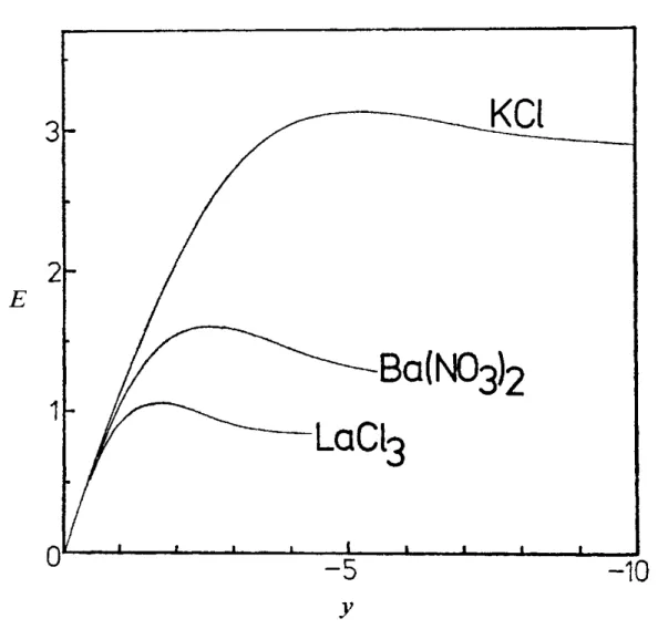
FIG. 6.-Effect of counterion valency on the form of the mobility against zeta potential curves, for ^{K a} = 5.

The marked effect of counter-ion valency on the mobility maximum is illustrated in fig. 6 where, for ^KU = 5, we plot p(5) for negative zeta potentials in 1 : 1 (KCl), 2 : 1 [Ba(NO,),] and 3 : 1 [La(CI),] electrolytes. The maximum in the mobility moves from y-5 in 1 : 1 electrolyte, to y-2.5 in 2 : 1 electrolyte and to y - 1.7 in 3 : 1 electrolyte. These values are in the ratio 1 :

t

t:.

It should be noted that the theories of Booth and Overbeek based on a perturba- tion expansion in powers of also reveal this mobility maximum. The numerical results of Wiersema strongly suggest the effect demonstrated here, but unfortunately the iteration scheme he used broke down at the value of 5 at which the maximum occurred (y-5 in 1 : I electrolyte, y-2.5 in 2 : 1 electrolyte). Indeed, the failure of the iterative scheme and the presence of the maximum are likely to be related.

Downloaded by Universitat Stuttgart on 25 March 2011 Published on 01 January 1978 on http://pubs.rsc.org | doi:10.1039/F29787401607

View Online

Electro-Hydrodynamical Model!

charged colloid!

!

n  driven system !

(external constant E –field)!

n  1 central Lennard-Jones ! (LJ) bead !

n  100 LJ monomers on the ! surface, connected to a network via FENE bonds!

n counterions: LJ beads!

simulation=> lattice (implicit) hydrodynamics Langevin MD + Lattice-Boltzmann algorithm periodic boundary conditions

Ewald sum: P³M

Ionic Distribution around the Colloid !

the ions within the shear plane renormalize the charge Z to Z_eff

Ionic Distribution around the Colloid!

Mobility as a Function of Charge Z!

Mobility is calculated at zero field with the Green- Kubo integral: linear regime

influence of comoving counterions counterion

condensation

Comparison to Experiments!

Z_Eff=20-30, R = 2.2 nm!

κ

= 4 π 

( n

+ n

Z

+ n

)

Salt and Concentration Effects!

Salt-free Simulations at finite Φ can be mapped to simulations including salt

Colloidal Electrophoresis!

Function Generator Sync. Output

for LED

CMOS

LED Indicator IR-blocking filter Fluidic Cell

A B

outlet inlet

AC E-Field

Comparison to experiments F. Kremer (Leipzig)

I. Semenov, S. Raafatnia, M. Sega, V. Lobaskin, C. Holm, F. Kremer. Phys. Rev. E 87(022302), 2013.

Simulation snapshot!

18!

10 ⁵ 10 ⁴ 10 ³ 10 ² 10 ¹ 6

4 2 0

Ionic Strength, [M]

reduced⇣-potential

Planar R=5 nm R=20 nm R=100 nm R=400 nm

Determination of zeta-potential!

20!

ILYA SEMENOV

PHYSICAL REVIEW E

potential drop between the bulk and the location of the shear plane, x

= 1.025 σ

. It has been checked that small variations in the location of the shear plane do not alter the results significantly. The electrophoretic mobility is eventually calculated using the SEM, taking as input the ζ potential obtained from the simulation and the experimental κ a value.

IV. RESULTS

Experimental and simulation results for the electrophoretic mobility as well as the experimentally measured phase angle are shown in Fig. 5 as a function of the ionic strength. As can be seen in Fig. 5(b), at most conditions the colloidal motion is out of phase (phase offset is ∼ 225 degrees) with respect to the electric field due to its negative surface charge. The decrease of the electrophoretic mobility with increasing ionic strength predicted by the SEM for all three valencies is observed in the

(a)

(b)

FIG. 5. (Color online) The electrophoretic mobility (a) and phase angle (b) vs. salt ionic strength of aqueous solutions of varying valency (KCl, CaCl

, and LaCl

). Squares represent the measured data, with error bars indicating the standard deviation.

The measurements for each valency are carried out with the very same negatively charged PS colloid (diameter: 2.23

strength is varied in the range 1–18 V/cm. The laser power is 0.2 W.

The simulation results with and without LJ attraction are shown via stars and triangles, respectively, connected by dotted lines for a guide to the eyes. In the monovalent case, the solid line represents SEM calculations based on GC solutions, whereas the dashed and dotted lines indicate SEM calculations using GC and spherical PB solutions, including the LJ attraction, respectively.

experiments; see Fig. 5(a). For monovalent salt, a maximum in the mobility is observed at low ionic strengths of ∼ 10

mol/l, which is in agreement with the SEM and previous findings for similar monovalent ionic solutions [9,47–49]. A less pro- nounced monotonic decrease of the mobility with increasing ionic strength is observed for CaCl

and LaCl

. In the case of trivalent salt, the experimental results show a mobility reversal, as can be inferred from the 180 degrees phase offset change, i.e. the colloid oscillates in phase with the electric field at I > 10

mol/l [Fig. 5(b)].

Using the experimentally determined colloidal surface charge density in the simulations, a quantitative agreement with the experiment is achieved for the monovalent salt in the peak area and the full curves are at least qualitatively repro- duced without further amendments to the restricted primitive model in the monovalent and divalent cases [see Fig. 5(a)].

However, no ζ potential (and hence mobility) reversal is observed in the trivalent case. This could have been expected, since in the strong coupling theory of Netz et al. [50] the Coulomb coupling parameter $ = 2π σ l

z

, where z denotes the counterion valency, needs to be larger than 10 to produce charge inversion by pure electrostatic correlation effects, while for the investigated trivalent salt system we have only $ = 1.7.

Obviously, the colloidal surface charge density is too low to bind a sufficient amount of trivalent ions electrostatically to produce the experimentally observed mobility reversal. This indicates the presence of other forces besides Coulombic attraction between the trivalent ions and the surface. In fact, specific interactions between La

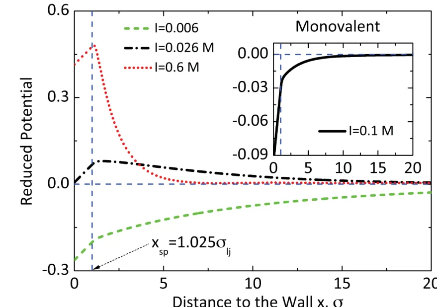
ions and Latex colloids have been reported by other authors [9,51–53]. Therefore, to model this ion-specific attraction the WCA interaction between the colloidal surface and the counterions is replaced by a full LJ potential. The resulting reduced electric potential profiles is shown in Fig. 6 for different ionic strengths. An attractive well depth of ε

= 4 k

T is found to be necessary in order to recover the mobility reversal in agreement with

FIG. 6. (Color online) Reduced electric potential (

BT

where

is the electric potential) profiles at different ionic strengths obtained from simulations of the trivalent case with full LJ interaction between the charged surface and the counterions. The position of the shear plane is taken to be at

1.025

from the solid surface. It is seen that for ionic strengths

10

mol/l, the

potential changes sign and, consequently, the mobility is reversed. In the inset, the reduced potential profile is shown for the monovalent case at ionic strength 10

mol/l. No mobility reversal is observed in this case.

022302-4

Experiment vs. Simulations!

21!

-6 -5 -4 -3 -2 -1 0 --3

--2 --1 -0 -1 -2 -3 -4 -5 -6

-5 -4 -3 -2 -1 0 -5 -4 -3 -2 -1 0

SCE, Experiment MD Sim, full LJ GC

GC+LJ

Spherical PB+LJ

Monovalent Divalent Trivalent

log Salt Ionic Strength [mol/l]

Mobility e*10-8 [m2 /Vs]

SCE, Experiment MD Sim, full LJ MD Sim, WCA

SCE, Experiment MD Sim, full LJ MD Sim, WCA

Ion specific interactions for La³⁺

Ka⁺ Ca²⁺ La³⁺

105 104 103 102 101

4

2

0

ReducedMobility

MONOVALENT

Spherical PB Experiment

105 104 103 102 101

Salt Ionic Strength [M]

DIVALENT

MD Sim Planar PB

105 104 103 102 101

4

2

0 TRIVALENT

Full LJ MD Sim Full LJ Planar PB

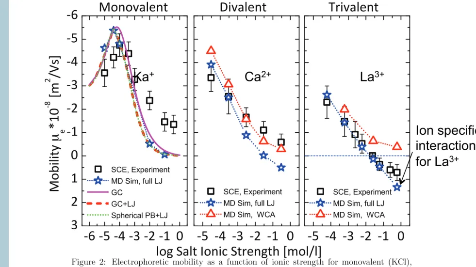
Figure 2: Electrophoretic mobility as a function of ionic strength for monovalent (KCl), divalent (CaCl₂) and trivalent (LaCl₃) salt solutions. Experimental results, black squares, are from Semenov et al.^10,31,32 for latex colloids of diameter 2.23 µm and surface charge density 0.31 µC/cm² ' 0.02 e/nm². Simulation results are represented via blue circles (WCA interaction) and red filled circles (full LJ interaction). The dashed and dotted lines represent calculations based on the numerical solution to the nonlinear planar and spherical PB, respectively. In the trivalent case, the red solid line represents the PB solution including the full LJ interaction between the counterions and the surface. Data taken from.¹⁰

Comparison to other Experimental Data!

22!

104 103 102 101

3 1 1 3 5 7

reducedmobility

MONOVALENT

Experiment Planar PB MD Sim WCA

105 104 103 102 101

salt ionic strength [M]

DIVALENT

105 104 103 102 101

3 1

1 3 5 7 TRIVALENT

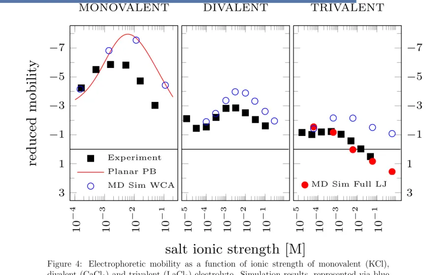
MD Sim Full LJ mobilities of latex colloids in mono-, di- and trivalent salt (KCl, CaCl2 and LaCl3 respec- tively) as a function of ionic strength using a Mark II microelectrophoresis apparatus. We compare our simulation results to their experimental data for a colloid of diameter 0.753µm and surface charge density 5.64µC/cm² ' 0.35 e/nm², see Fig. 4. Due to the large size of the colloid in comparison to the Debye length in the considered range of salt concentrations, 12 < R < 3.91 ⇥10², the planar geometry inherent in our simulation technique is also appropriate for this system.

104 103 102 101

1 1 3 5

ReducedMobility

MONOVALENT

Experiment Spherical PB

105 104 103 102 101

Salt Ionic Strength [M]

DIVALENT

MD Sim Planar PB

105 104 103 102 101

1 1 3 5 TRIVALENT

Full LJ MD Sim Full LJ Planar PB

Figure 4: Electrophoretic mobility as a function of ionic strength of monovalent (KCl), divalent (CaCl2) and trivalent (LaCl3) electrolyte. Simulation results, represented via blue (WCA) and red filled circles (full LJ), are compared to the experimental results of Elimelech et.al indicated by black squares. Experiments were done by Elimelech et al.⁶ with latex colloids of diameter 0.753 µm and surface charge density 5.64 µC/cm² ' 0.35 e/nm². The dashed and dotted lines represent calculations based on the numerical solution to the nonlinear planar and spherical PB, respectively. In the trivalent case, the red solid line represents the PB solution including the full LJ interaction between the counterions and the surface.

17

Conclusions!

• Successful mapping of simulations of charged colloidal electrophoresis onto experimental values

• Colloidal concentration can be mapped on salt concentration

• Intriguing minimum observed in µ_red as function of κR

• SEM works well, even for multivalent salt solutions if combined with Simulations for determining the zeta potential

• In specific effects (non-electrostatic attraction) might be important for some ion species (here La³⁺)

24!

Electrophoresis of Polyelectrolytes

Christian Holm

Institut für Computerphysik, Universität Stuttgart Stuttgart, Germany

Outline!

n 

Coarse-grained simulation model for electrophoresis with and without HI!

n 

Results on diffusion & mobility compared to experiments!

n 

Effective charge estimators!

n 

Effective friction of polyelectrolytes in free- solution electrophoresis!

n 

ELFSE!

n 

Electrophoresis of charged colloids!

Why care about electrophoresis?!

n  Electrophoretic separation of DNA!

n  Crucial step is gene analysis!

n  Yields characteristic genetic finger prints!

n  Today: Gel Electrophoresis based on entanglement !

n  Widely applicable and reliable!

n  Slowed down dynamics leads to long elution times!

n  Future: Novel separation techniques based on hydrodynamic and chemical interactions!

n  Micro-fluidic devices with structured surfaces!

n  On-going design and development process!

First Goal: Understand free-flow Electrophoresis

Free-Flow Electrophoresis!

n 

Charged polymers move in solution under the influence of an external electric field!

n 

Local force balance leads to constant velocity!

n  Electrical driving force!

n  Solvent friction force!

n 

Electrophoretic mobility µ!

n  Size dependence of µ (N)
 determines separation

process!

(N)

(N)

Short and long polyelectrolytes!

n 

Short PE chains:!

n  Extended rod-like conformation!

n  Length dependent mobility!

n 

Long PE chains:!

n  Random coil conformations!

n  Screening of long range hydrodynamic interactions!

n  Length independent mobility (free-draining)!

N

µ(N)

N_FD

Free- draining

Crossover:

§ DNA: N_FD ~ 170 bp

§ PSS: N_FD ~ 100 units

Experimental observations:

Short and long polyelectrolytes!

n 

Short PE chains:!

n  Extended rod-like conformation!

n  Length dependent mobility!

n 

Long PE chains:!

n  Random coil conformations!

n  Screening of long range hydrodynamic interactions!

n  Length independent mobility (free-draining)!

N

µ(N)

N_FD

Free- draining

Crossover:

§ DNA: N_FD ~ 170 bp

§ PSS: N_FD ~ 100 units

Experimental observations: Not understood

Model!

n 

No chemical
 details!

n  Charged
 subgroups
 connected


along a backbone by elastic springs!

n  Ions modeled as free mobile charges !

n 

Implicit solvent model

n  continuous dielectric background !

n  Explicit charges treated with full electrostatics via P3M in p.b.c.!

n  Explicit hydrodynamics by frictionally coupling the beads to a Lattice-Boltzmann fluid!

n  Can simulate with HI and without HI (Langevin)!

LB-Hydrodynamics!

• 

Lattice Boltzmann equation!

•  streaming and collision!

•  discrete set of velocity populations!

•  D3Q18 scheme!

•  hydrodynamic fields
 from populations!

32!

Hydrodynamics via LB!

n 

Frictional coupling of MD particles to Lattice Boltzmann fluid [1]!

n  Modified Langevin equation:!

n  Momentum exchange between immersed particles and fluid!

n  Total momentum conservation!

Hydrodynamic interactions

[1] P. Ahlrichs and B. Dünweg. International Journal of Modern Physics C, 9:1429-1438, 1998.

Current D3Q19 Version with correct fluctuation spectrum due to Schiller, Duenweg implemented in ESPResSo

33!

Observables!

n 

Zero-field mobility (Green-Kubo):

µ = 1

3k

T q

r

v

(0) ⋅ r

v

( τ ^{) d} τ

0

∞ i

∫

∑

n 

(Self-)Diffusion D

n 

Electrophoretic mobility µ

34!

Simulation parameters!

n  Mapping on sulfonated polystyrene (PSS)!

n  All beads have diameter of 2.5 Ångström!

n  Chain length N=1 …64!

n  l_b = 7.1 Ångström (H₂O at 20° C)!

n  Monomer concentration 100 mMol!

n  No added salt!

n  Experimental conditions:!

n  Böhme, Scheler, IPF Dresden, PFG-NMR!

n  H. Cottet, CNRS Montpellier, Cap. Elec.!

Results 1: Diffusion!

K. Grass, U Böhme, U. Scheler, H. Cottet, and C. Holm, Phys. Rev. Lett. 100, 096104 (2008)

Electrophoretic mobility!

K. Grass, U Böhme, U. Scheler, H. Cottet, and C. Holm, Phys. Rev. Lett. 100, 096104 (2008)

No HI!

Effect of HI

with! without

hydrodynamical interactions (HI)!

Independent. of c_s!

Salt dependence c _s of Mobility !

Maximum reproduced No maximum

Polyelectrolyte-ion-complex!

E

Hydrodynamic Friction!

n 

Important quantity to characterize PEs!

n 

Effective friction for polymers!

n 

Obtainable from mobility measurements!

Q1: How to estimate the effective charge?

Q2: Can we use Γ

= Γ

to measure Q

_

_

_

3 Estimators for Q _eff!

(1)  Ion velocity distribution to find co- moving counter ions !

(2)  Calculation from Langevin (no HD) mobility !

(3)  Counter ions within 2σ of PE chain!

Co-Moving Counter Ions!

n 

Co-moving counter ions reduce effective charge of PE-Ion complex!

n 

Look at the ion velocity distribution to find

co-moving counterions!

Ion Velocity Distribution!

Simulations with and without HD yield almost identical threshold

=>

similar Qeff

v_Ion: relative velocity to center of mass (PE + CI) frame

Langevin Simulation (No HI)!

n 

The mobility measures the combined

movement of PE and co-moving counter ions!

n 

Local friction of each particle is given in

Langevin simulation as!

Estimator Comparison!

Qeff(3) > Qeff(2) ≈ Qeff(1)

Manning fraction f_M = 1-b/λ_B based on one infinite rod at infinite dilution dynamic Q_eff= static Q_eff

Effective Friction!

PE effective friction deviates from single chain D for

Debye length ≈ hydrodynamic screening length

_ _ _ _

Effective Charge and Friction!

Constant friction and charge per monomer for long PEs.

Debye length ≈ hydrodynamic screening length

_

3 Estimators for Q _eff!

(1) Calculation from Langevin mobility (no HI) !

(2) Ion velocity distribution to find co- moving counter ions!

(3) Counter ions within 2σ of PE chain!

Ion velocity with respect to CM!

Effective charge vs. N!

Only the dynamical estimators Q⁽¹⁾_eff and Q⁽²⁾_eff are compared

Effective charge estimators Q⁽¹⁾_eff and Q⁽²⁾_eff are numerically equivalent! No dependence on hydrodynamical interactions, weak salt dependence for small N, Q_eff is independent of

Static effective charge Q ⁽³⁾ _eff!

50!

Contrary to the dynamical estimators we observe a strong salt dependence

Effective friction vs. N!

Zimm (?) scaling with! Rouse (?) scaling without hydrodynamical interactions!

versus!

Effective friction vs. chain length!

With! Without

hydrodynamical interactions.!

For large N Γ/Ν = constant

!

Independant. of c_s Hydrodynamic shielding

Hydrodynamic coupling scheme !

Influence of surrounding ions on hydrodynamic screening length

Debye length ≈ hydrodynamic screening length

unscreened! medium screening by counterions!

large screening by counterions!

Intermediate conclusion on FSE!

n  Coarse-grained MD with full electrostatic and explicit hydrodynamic interactions reproduce experimental results on bulk electrophoresis of polyelectrolytes, with and without salt!

n  Mobility maximum due to hydrodynamic shielding !

n  Dynamic charge estimators do not depend on HI, and are

independent of salt (the static one is, however, salt dependent!)!

n  Effective friction is strongly influenced by co-moving ions and salt concentration: !

n  Hydrodynamic shielding for short N, constant friction per monomer for long chains due to hydrodynamic screening!

• K. Grass, U. Böhme, U. Scheler, H. Cottet, C. Holm, Phys. Rev. Lett., 100, 096104 (2008).

• K. Grass, C. Holm, J. Phys.: Condens. Matter 20, 494217 (2008).

• K. Grass, C. Holm, Soft Matter 5, 2079 (2009).

How to separate long chains?!

n 

Attaching a label to the PE changes the scaling of effective friction („Molecular parachute“) ELFSE (End-Labeld Free Solution Electrophoresis) principle!

n 

Size-dependent free-solution mobility of long PE chains!

• Mayer, P., et. al.; Anal. Chem.

1994, 66, 1777-1780!

• Ren, H., et. al.; Electrophoresis 1999, 20, 2501-2509!

End-labeles!

• Linear tags

• Branched tgs

• Micellar tags

Mobility influenced by label!

n End-labeling restores size dependence of mobility !

Theoretically expected slowdown!

§ 

Calculate persistence length


§ 

Calculate α from simulation according to!

• Desruisseaux, C. et. al.; Macromolecules 2001, 34, 44-52!

Slow down as expected!!

λ_D

Conclusions on ELFSE!

• 

ELFSE works according to the theoretical predictions!

• 

Size dependant sparation can be pushed to longer chain lengths!

• 

The insight gained by analyzing this process can lead to optimized experimental setups!

n  For more details see:

K. Grass, C. Holm, G. Slater, Macromolecules, 42, 5352-5359 (2009)

!

Governing Physics for Bare Colloids

⇥_s ⌅⇧u

⌅t = r²⇧u r⇧ P

XN

j=1

n_jz_jer⇧ ⇤ Stokes equation:

j(~u ~v_j) z_jer~ k_BT r~ log n_j = ~0 Poisson-Nernst-Planck equation:

r~ · ~u = ~0 Incompressibility:

Solvent’s density, velocity and viscosity

⇥_s, ⇤u, :

P : ^Pressure

V : Particle’s velocity

r~ :Electric field due to ions of charge and concentration

and the applied field z_j n_j

j : ionic drag coefficient

⇥

⌅⇧ u

⌅ t = r

⇧ u r ⇧ P +

l

( V ⇧ ⇧ u)

| {z }

drag force of the layer

X

j=1

n

z

e r ⇧ ⇤ The Darcy-Brinkman equation:

l² : permeability of the grafted polymer layer

Brinkman length related to the monomer distribution, decreases with increasing monomer density

Governing Physics for Soft Colloids

j

(~ u ~ v

) z

e r ~ k

T r ~ log n

= ~ 0 Poisson-Nernst-Planck equation:

r ~ · ~ u = ~ 0 Incompressibility:

l(r) :

Monday, July 7, 2014

Soft Colloid Electrophoresis

• Canonical ensemble (NVT)

• L: Simulation box size (L=48σlj)

• Raspberry-like colloid

• ^Rcol: colloid radius (R=3σlj)

• ^Qcol: colloid charge

• N: number of grafted polymers (N=20)

• M: degree of polymerization of each chain (M=20)

• H: layer thickness ~ 4.5σlj

• λ: fraction of charged monomers

• ^cs: monovalent salt concentration

• ^λD: Debye length

• HI via LB fluid

Hill’s numerical solver based on Darcy-Brinkman formalism

Monomer density parameters found from fit to simulation

* Hill et al., Colloids and Surfaces A: Physicochem. Eng. Aspects 267 (2005) 31–49

µ_red = 3 2

⌘e

✏_rs✏k_BT µ_e

Mobility of Neutral Soft Colloid

10 ³ 10 ² 10 ¹ 10⁰ 0.5

0 0.5 1

c_s/M µ red

Simulation Theory

10⁰ 10^{1 D}/

= 0.1 Qcol = 40 e Qnet = 0 e

Monday, July 7, 2014