Constraints on promptly decaying supersymmetric particles with lepton-number- and R-parity-violating interactions using Run-1

ATLAS-CONF-2015-018 20May2015

ATLAS NOTE

ATLAS-CONF-2015-018

19th May 2015

Constraints on promptly decaying supersymmetric particles with lepton-number- and R-parity-violating interactions using Run-1

ATLAS data

The ATLAS Collaboration

Abstract

In this document, a selection of ATLAS searches for supersymmetry (SUSY), mostly op- timised for R-parity-conserving SUSY, are reinterpreted in new R-parity-violating SUSY models where an unstable neutralino decays promptly to leptons and/or jets. All forms of renormalisableR-parity-violating interactions with lepton-number violation are considered.

The production of squarks and gluinos is constrained for different neutralino masses and de- cay modes. In most cases lower limits on the squark and gluino masses ofm & 1 TeVare obtained; exceptions to this rule are located and discussed. Additionally, bilinear R-parity violation is considered in a model with a natural SUSY spectrum with light third-generation squarks and higgsinos. Only a small portion of the explored parameter space remains unex- cluded, wherem_q˜L,3 > 810 GeV.

c

2015 CERN for the benefit of the ATLAS Collaboration.

Reproduction of this article or parts of it is allowed as specified in the CC-BY-3.0 license.

1. Introduction

The search for new particles and phenomena not described by the Standard Model of particle physics (SM) is one of the primary objectives of the ATLAS experiment [1]. Weak-scale supersymmetry (SUSY) is a well-motivated and well-studied example of a model used to guide many of these searches [2–10].

In this document, new constraints are set on SUSY models in the presence of lepton-number violating interactions (/L) that are present in generic SUSY models with minimal particle content. These inter- actions, together with similar baryon-number-violating interactions (/B), are described by the following superpotential terms:

WLRPV/ = 1

2λ_{i j k}L_iL_jE¯_k +λ⁰_{i j k}L_iQ_jD¯_k+_iL_iH₂, (1a) W_BRPV/ = 1

2λ⁰⁰_{i j k}U¯_iD¯_jD¯_k. (1b)

In this notation, L_i andQ_i indicate the lepton and quark SU(2)-doublet superfields, respectively, while E¯_i, ¯U_i and ¯D_i are the corresponding singlet superfields. The indicesi, jandk refer to quark and lepton generations. The Higgs SU(2)-doublet superfield H₂ contains the Higgs field that couples to up-type quarks. The λ_{i j k}, λ⁰_{i j k}and λ⁰⁰_{i j k} parameters are new Yukawa couplings, while the _i parameters have dimensions of mass. The terms in Eq. (1) are forbidden in many models of SUSY by the imposition of R-parity conservation in order to prevent rapid proton decay [11–15]. However, proton decay can also be prevented by suppressing only one ofW_LRPV/ orW_BRPV/ , in which case someR-parity-violating (RPV) interactions remain in the theory.

Introducing non-zero RPV couplings into supersymmetric models can significantly weaken mass and cross-section limits from collider experiments and also provide a rich phenomenology, see e.g. Refs. [16–

20]. Most relevant is the fact that the lightest supersymmetric particle (the LSP) is unstable and decays to SM particles via the interactions in Eq. (1), rather than escaping unseen as predicted by models that conserve R-parity. The LSP lifetime, τ_LSP, is not predicted in general; we focus on prompt decays of a neutralino LSP, meaning that the decay distance is not resolved from the point of production by the considered ATLAS searches. The upper limit of what may be regarded as prompt is analysis-dependent, but as a general guideline, channels requiring the explicit reconstruction of a lepton require τ_LSP . O(1 ps) to satisfy typical requirements on the lepton’s impact parameter, while channels with a lepton veto have sensitivity up to lifetimes of approximately 1 ns [21]. A systematic phenomenological overview of possible signatures specific to a particular RPV scenario is given in Ref. [20], which goes through all possible mass orderings and the dominant decay signatures.

Existing searches for supersymmetry with L/ RPV are reviewed in Sect.1.1. These include constraints on decays via the first (LLE) operator in Eq. (1a), but only in the case where a single RPV coupling is¯ dominant, which limits the possible event signatures. In spite of the rich phenomenology, prompt decays via the second (LQD) term of Eq. (1a) have so far been considered by ATLAS only for the specific case of¯ a top-squark LSP [22]. Limits have previously been set on decays via the third, bilinear, term of Eq. (1a), but only in the case of the highly constrained mSUGRA model. In this note, the scope of constraints set by ATLAS on lepton-number-violating SUSY decays is expanded by considering nearly all possible decay patterns of a neutralino LSP allowed by Eq. (1a). The baryon-number-violating interactions of Eq. (1b) are not considered, as they have already been well-addressed by ATLAS searches [23], and are strongly constrained if lepton-number-violating interactions are also allowed.

A total of four models are considered in this note. Three are simplified models, and allow the neutralino LSP to decay via theLLE¯ orLQD¯ operators. We focus on the production of squarks and gluinos, which will be produced more abundantly at the LHC than other SUSY particles if they are not too massive. The new results obtained here can inform search strategies for Run-2 and indicate where specific optimisations may be required. In addition, the existing ATLAS constraints on gluino production withLLE-mediated¯ LSP decays are strengthened by including results from other searches that did not previously consider this scenario. In the case of bilinearR-parity-violation (bRPV), the connection between thebRPV couplings and neutrino masses is used to require that all model parameters are consistent with neutrino data [24].

Generic squark and gluino production is already highly constrained in this case (see Sect.1.1), therefore a natural SUSY model is considered, with light top squarks and higgsino-like neutralino LSPs, within the framework of the phenomenological minimal supersymmetric Standard Model (pMSSM) [25].

The searches used to constrain these models all use 20.3 fb⁻¹ of pp collision data with √

s = 8 TeV collected in 2012. Many of the searches used were optimised for R-parity-conserving (RPC) SUSY models but nevertheless can tightly constrain RPV scenarios. A short overview of which analyses are used to constrain which models is given in Sect.2, after the current constraints on RPV SUSY production at the LHC are reviewed. The models are described in more detail in the following sections, together with the exclusion limits obtained from the ATLAS data. TheLLE¯ andLQD¯ models are covered in Sect.3, while Sect.4concerns thebRPV model. Finally, the conclusions are presented in Sect.5.

1.1. Existing constraints onL-violating RPV SUSY

In this section, constraints on SUSY production with RPV decays by the ATLAS [1] and CMS [26]

collaborations are described, focusing on the lepton-number-violating interactions of Eq. (1a).

The ATLAS search for events with four or more charged leptons [27] has constrained models withLLE¯ couplings. Strong constraints were placed when the λ₁₂₁ or λ₁₂₂ terms dominate, while less stringent limits were found for tau-rich events produced by the λ₁₃₃ or λ₂₃₃ terms. Additionally, a search for non-prompt signatures included channels with displaced charged lepton pairs, probing smaller values of λ₁₂₁ andλ₁₂₂ couplings [28]. Multi-lepton searches forLLE-type scenarios have also been performed¯ by CMS [29,30], including extensions into non-prompt decays [31]. Stop pair production was probed by CMS using multi-lepton events with jets tagged as originating fromb-quark decays (b-jets), constraining signatures based on λ₁₂₂ and λ₂₃₃ decays [32] and also λ₁₂₃-related models [33]. Searches for LLE-¯ related signatures were also performed at the Tevatron’s D0 and CDF experiments [34, 35] and by the LEP collaborations [36,37].

Searching for effects fromLQD¯ couplings, ATLAS has placed constraints on non-prompt decays leading to a multi-track displaced vertex [28]. A search for ˜t₁t˜₁ → b`b`events also constrained prompt decays of the top squark viaLQD¯ couplings [22]. A similar model with non-prompt decays was investigated by CMS [38]. The CMS search for events with multiple leptons andb-jets [32] has been interpreted to constrain decays mediated byλ⁰₂₃₃while Ref. [33] also examinedλ⁰₂₃₁decays. Furthermore the search in Ref. [39] constrained models with non-zeroλ⁰₃₃₃andλ⁰_{3j k} (withj,k =1,2), investigating signatures from τ-leptons andb-jets.

Assuming abRPV extension of the mSUGRA model, limits on the underlying mSUGRA mass parameters m₀ andm_1/2 were obtained in several ATLAS analyses. The most sensitive channels required jets in addition to one or more charged leptons, where the charged leptons may be electrons and muons [40,41], or hadronically decaying taus [42].

Distinct signatures from resonant sparticle production with subsequent decay are possible for a combina- tion of non-zeroLQD¯ andLLE¯couplings. The ATLAS collaboration performed a dedicated search [43]

for a heavy narrow resonance decaying toeµ, eτ, or µτ assuming non-zero λ⁰₃₁₁ in combination with non-zero λ₁₃₂, λ₁₃₃, or λ₂₃₃, respectively. The eµ case was also considered by CMS [44], and both searches significantly improve previous constraints from CDF [45] and D0 [46]. Using the search chan- nel for same-sign muons and at least two jets as motivated by resonant smuon production, the CMS collaboration obtained limits on the couplingλ⁰₂₁₁in the mSUGRA framework [47].

2. Overview of reinterpreted analyses

This section summarises the most relevant aspects of the different analyses used for constraining theR- parity violating models considered in this note. Since all the selection criteria used have been defined in detail in the original analysis papers, only the most relevant selections are outlined in what follows. The analyses make use of three types of event selection:

Signal regions (SRs) are used to search for signs of a SUSY signal.

Control regions (CRs) are used to determine the rate of SM background processes in the SRs.

Validation regions (VRs) are used to check the predictions made using the CRs.

When each analysis was designed, it was checked that the CRs and VRs were free of SUSY signal events, for the particular models under consideration at the time. This may not be true when new models are considered, so the CR and VR contamination must be checked anew. Increased contamination has different potential consequences, depending on where it occurs. VR contamination will not directly affect a reinterpretation of a search, but it potentially invalidates the original SM background prediction, and should therefore be no larger than the associated uncertainty. As the CRs are used to estimate the rate of SM processes, the estimated SR background will change if a significant fraction of CR events can be attributed to signal. For this reason, the contribution of signal is accounted for in each CR and the SM background recalculated when setting new limits. Relevant CRs and VRs are also listed in the analysis descriptions below.

It has been found that many of the considered searches are sensitive to more than one model, and that most models can be constrained by more than one search. To help guide the reader, Table1briefly summarises which analyses are used to constrain which RPV SUSY models. The precise descriptions of the models considered, and specific details of the associated CR and VR contamination, can be found in Sects.3and 4.

In the earlier descriptions of the analyses that are considered herein, the term “lepton” has several different meanings depending on the nature of the paper. Here and in the following, it refers to any charged or neutral lepton of any generation. The corresponding definitions of charged or neutral leptons also refer to leptons of any generation. The term “light lepton” is used to indicate only electrons and muons.

2.1. Four-lepton analysis

The four-lepton (4L) analysis [27] was designed to be sensitive to SUSY models with non-zeroLLE¯RPV couplings, as well as RPC SUSY models that predict events with high numbers of charged leptons in the

Simplified models pMSSM

LLE¯ LQD¯ LQD¯ bRPV

˜

gg˜ g˜g˜ q˜q˜ Short name Ref. 4q,4`,2ν 8q,2(`/ν) 6q,2(`/ν)

4L [27] X

SS/3L [40] X ♦ X

1L [41] X X ♦

0L 2–6 jets [48] X X

0L 7–10 jets [49] X

Table 1: Overview of analyses used to constrain the RPV models in this note. The signature descriptions are indicative only, and the reader is referred to the analysis documentation for further details in each case. Filled cells indicate where limits have been obtained by a particular analysis for a particular model. In cells with a lozenge (♦), the resulting limits are surpassed by other channels and there is no contribution to the final results from that analysis. For the simplified models, an indication is given of the nominal event signature, whereq,`andνrefer to quarks, charged leptons and neutrinos, respectively, of any generation.

SR name N(e/µ) N(τ) E_T^miss[GeV] orm_eff [GeV]

SR0noZb ≥ 4 ≥ 0 ≥75 or ≥600

SR1noZb =3 ≥ 1 ≥100 or ≥400

SR2noZb =2 ≥ 2 ≥100 or ≥600

Table 2: Definitions of the most relevant signal regions from the 4L analysis [27].

final-state. It requires at least four charged leptons in every signal event, at least two of which must be light leptons. The events are separated into signal regions based on the number of light leptons observed, and the presence or absence of aZboson candidate among the pairs of light leptons. Final suppression of the SM background is made using the missing transverse momentum (the magnitude of which is denoted E_T^miss) and the effective mass (m_eff), defined in this case as the scalar sum of the E_T^miss, the p_T of all selected charged leptons and the p_T of reconstructed jets with p_T > 40 GeV.1 No explicit requirement is made on reconstructed jets, ensuring that the search is sensitive to both strong and electroweak SUSY production processes.

Of the nine SRs used in the 4L analysis, only the three described in Table 2are relevant to this note.

In all cases, events with a pair of light leptons forming a Z boson candidate are vetoed, and possible Z → `<sup>+</sup>`⁻γ and Z → `<sup>+</sup>`⁻`<sup>+</sup>`⁻ candidates are also rejected. Additionally, either high E_T^miss or high m_eff is required – thus, a selected event may have one quantity below the threshold, but never both. The resulting SM background is very low, between about 1.4 and 3 events for the SRs considered here. As the three SRs used here have mutually exclusive selection criteria, they are statistically combined when setting constraints on the specific SUSY models.

In the 4L analysis, CRs are used to estimate the background contribution from non-prompt and fake

1ATLAS uses a right-handed coordinate system with its origin at the nominal interaction point (IP) in the centre of the detector and thez-axis along the beam pipe. The x-axis points from the IP to the centre of the LHC ring, and the y-axis points upward. Cylindrical coordinates (r, φ) are used in the transverse plane,φbeing the azimuthal angle around the beam pipe.

The pseudorapidity is defined in terms of the polar angleθasη=−ln tan(θ/2). The transverse momentum of a particle is denotedp_T= q

p²_x+p²_y.

SR Leptons N_b−jets Other variables m_eff

SR3b SS or 3L ≥3 N_jets≥ 5 m_eff >350 GeV

SR1b SS ≥1 N_jets≥ 3,E_T^miss >150 GeV, m_eff >700 GeV m_T >100 GeV, SR3b veto

SR3Lhigh 3L - N_jets ≥4,E_T^miss >150 GeV, SR3b veto m_eff >400 GeV Table 3: Definitions of the most relevant signal regions from the SS/3L analysis [40].

leptons. They have the same kinematic requirements as the corresponding signal regions, but one or two of the four charged leptons must fail the standard isolation or other identification criteria normally used.

Also, VRs are used to check the background estimates. In events with aZboson veto, the VR events must satisfyE_T^miss < 50 GeV andm_eff <400 GeV. The possible contamination of these control and validation regions by theLLE¯ model considered in this note was already investigated in Ref. [27], and found to be negligible.

2.2. SS/3L analysis

The SS/3L search [40] requires two light leptons with the same electric charge or three light leptons in conjunction with requirements on the number of jets. It is aimed at SUSY models where pair-produced Majorana particles (e.g. gluinos) can decay semileptonically with a large branching ratio. The effective mass, m_eff, is a key discriminating variable, defined in the SS/3L analysis as the sum of E_T^miss and the p_T values of the leptons and jets (with p_T > 40 GeV). The two leading light leptons have to fulfil p_T >20 GeV andp_T >15 GeV, respectively. If the lepton contains a third light lepton withp_T> 15 GeV the event is regarded as three-lepton event, otherwise it is a two-lepton event.

Five different signal regions are defined, where all details are described in the corresponding paper. The most relevant SRs for the results in this analysis are summarised in Table3. SR3b and SR1b use leptons, the presence ofb-jets and largem_eff to suppress the SM background. There is no explicitE_T^miss require- ment in SR3b, which means it does not depend on the assumption of a stable LSP escaping the detector unseen. SR1b additionally uses the transverse mass, m_T, to reject background events with W bosons, defined as

m_T = q

2p<sup>`</sup><sub>T</sub>E<sub>T</sub><sup>miss</sup>(1−cos[∆φ(~`,p^miss_T )]), (2) wherep_T^`is the larger of thep_Tvalues of the two charged leptons, andp^miss_T is the missing transverse mo- mentum vector. The SR3Lhigh selection requires a third light lepton for additional background rejection, in addition to requiring at least four high-pTjets. All SRs for the SS/3L search have been designed to be statistically independent, and are combined to improve the overall sensitivity.

Several VRs are used to check the quality of the background estimates used in the SS/3L search. Of par- ticular interest are those regions dedicated to rare processes, which have a relatively low number of events and are potentially susceptible to contamination from a SUSY signal. Events with same-sign muons and two b-jets are used to check the t¯tW background, while events with three light leptons (including a Z candidate) and at least oneb-jet are used to validate thet¯t Zbackground component. Finally, events with same-sign muons and nob-jets are used to check theW Zbackground.

3-jet 5-jet 6-jet

N_lep =1 =1 =1

p^lep1_T [GeV] >25 > 25 >25

p^lep2_T [GeV] <10 < 10 <10

N_jet ≥3 ≥5 ≥6

p^jet_T [GeV] >80, 80, 30 > 80, 50, 40, 40 ,40 >80, 50, 40, 40, 40 ,40 p_T^{5th jet} <40 GeV p_T^{6th jet} <40 GeV

E_T^miss[GeV] >300 > 300 >250

m_T[GeV] >150 > 150 >150

E_T^miss/m^excl_eff > 0.3 – –

m^incl_eff [GeV] >800 > 800 >600

shape fit variable m^incl_eff m^incl_eff E_T^miss binning: bin size 4 bins: 200 GeV 4 bins: 200 GeV 3 bins: 100 GeV

Table 4: Definitions of the most relevant signal regions from the 1L analysis [41].

2.3. Strong production with leptons analysis

The analysis in Ref. [41] is designed to be sensitive to a wide variety of SUSY models where light leptons may be produced, for example viaW → `ν decays. It considers a variety of selections, requiring one or two light leptons with opposite charge. In the context of the models considered in this note, only the regions requiring one high-p_T(> 25 GeV) lepton are considered, and for this reason it is referred to here as the 1L analysis. A summary of the SR selection criteria can be found in Table4. The transverse mass m_T is defined using Eq. (2) applied to the lepton to reject events containing aW boson. The inclusive effective mass (m^incl_eff ) is the scalar sum of thep_Tof the lepton, the jets (with p_T > 25 GeV) and theE_T^miss:

m^incl_eff =p_T^`+

Njet

X

j=1

p^jet_{T j}+E_T^miss. (3)

Furthermore the ratioE_T^miss/m^excl_eff is computed, where the exclusive effective mass,m^excl_eff , is defined in a similar way tom^incl_eff but using only the three leading jets. The SRs are each binned in one variable and are statistically independent. They are statistically combined to give improved sensitivity when excluding a particular SUSY model.

Control regions are used in the 1L analysis to constrain the dominant background processes, such ast¯t, using events with lower values ofE_T^miss andm_T. In order to test the extrapolation from the CRs to the SRs, which is based on simulated events, two validation regions are also defined for each signal region.

One VR extends to highE_T^miss, while the other reaches towards higherm_T, starting from thet¯tandW+jets control regions. The samem_eff selections as in the SRs are applied in every case.

2.4. Zero-lepton, 7–10 jets analysis

The 0L 7–10 jets analysis [49] was designed to be sensitive to SUSY events with high jet multiplicities and no isolated light leptons. Compared to many SUSY searches, only a relatively loose requirement is

j50 j80 8j50 9j50 ≥10j50 7j80 ≥8j80

Jet|η| <2.0 <2.0

Jetp_T >50 GeV > 80 GeV

N_jet =8 =9 ≥10 =7 ≥8

b-jets 0,1,≥ 2 0,1,≥2 — 0,1,≥2 0,1,≥2 E^miss_T /√

H_T ≥4 GeV^1/2 ≥ 4 GeV^1/2

Table 5: Definitions of the 13 signal regions of the multi-jet+flavour stream of the 0L 7–10 jet analysis [49]. The signal regions are separated into two groups, labeled j50 and j80. Signal regions within each group are statistically combined, and the most sensitive SR group is used to set model-dependent limits.

Requirement 5j 6jl 6jm 6jt+

N_jet≥ 5 6 6 6

E_T^miss/m_eff(N_jet) > 0.2 0.2 0.2 0.15 m_eff(incl.) [GeV]> 1200 900 1200 1700

Table 6: Final kinematic selections for the most relevant signal regions from the 0L 2–6 jets analysis [48]. Selection criteria common to these four signal regions are described in the text.

made on theE_T^miss. Example SUSY models targeted by this analysis include gluino pair production where each gluino decays tott¯χ˜⁰₁, and RPV SUSY with decays via the baryon-number-violating operator in Eq. (1b).

The signal regions of this analysis are split into two streams, denoted “multi-jet+flavour” and “multi-jet + M_J^Σ”. The multi-jet + M_J^Σ stream makes use of large-radius (R = 1) jets reclustered from smaller R= 0.4 anti-k_t jets. It is not used in this note because preliminary studies indicated that the multi-jet+ flavour stream is expected to be at least as powerful in all of the models considered. The signal regions of the multi-jet+flavour stream are listed in Table5. There are two groups of disjoint selections, which differ in the minimum jet p_T requirement, either p_T > 50 or 80 GeV. To constrain a specific model, all SRs within each group are statistically combined, and the group with the best expected limit is used.

As with the other analyses, control regions are used to estimate the main background sources. In partic- ular, events with five or six jets are used to estimate the multi-jet background by extrapolating from low to high values of E_T^miss/√

H_T, where H_T is the scalar sum of the p_T of all jets with p_T > 40 GeV and

|η| < 2.8. Validation regions with one isolated light lepton are also defined to check the accuracy of the background estimates fort¯t,W+jets and Z+jets events.

2.5. Zero-lepton, 2–6 jets analysis

The last analysis used in this note is a generic search for squark and gluino production in events with large E_T^miss, no isolated electrons or muons and at least 2–6 jets [48]. It is designed primarily to be sensitive to the RPC decays of squarks and gluinos, in cases where isolated light leptons are not produced, e.g.

˜

gg˜ →qqq¯ q¯χ˜⁰₁χ˜⁰₁. A total of fifteen signal regions are defined, which vary in the minimum jet multiplicity requirement and other kinematic criteria. Of these SRs, only four are relevant for the signals considered here. These four all require at least five jets withp_T > 60 GeV (all but one require at least six jets), and

at least one jet withp_T > 130 GeV. Additionally, the magnitude of the missing transverse momentum must be greater than 160 GeV, and it must not be aligned in the transverse plane with any jet that has p_T > 40 GeV to reduce the effect of mismeasured jet momenta. Further selections applied to individual SRs are listed in Table6, which include two variations on the effective mass:

m_eff(N_jet) =E_T^miss+

Njet

X

j=1

p^jet_{T j}, (4)

andm_eff(incl.) =E_T^miss+ X

pT>40 GeV

p^jet_T , (5)

whereN_jetrefers to the number of jets required by the region, i.e. in this case five or six. The SRs are not statistically independent, and so constraints on any given SUSY model are obtained only with the region that has the best expected sensitivity.

For each SR, four control regions are used to estimate the contributions from different SM background processes. The multi-jet contribution is estimated using events where the E_T^miss vector is aligned with one of the jets, and also theE_T^miss/m_eff(N_jet) selection is inverted (the control region with this selection is called CRQ in Ref. [48]). The contributions of events withW andt¯tproduction are estimated in events with one isolated light lepton and ab-jet veto or tag, respectively (CRW and CRT). Finally,Z(→νν)+jets events are estimated using events with a single isolated photon (CRγ).

3. LL E ¯ and LQ D ¯ simplified models

3.1. Introduction

The simplified models with R-parity-violating SUSY decays are based on those used in the 4L SUSY search described in Sect. 2.1 [27]. Equivalently, they are similar to the simplified models with RPC squark and gluino production with a neutralino LSP used in, for example, the 0L 2–6 jets search [48], except that the addition of the RPV couplings now allow the LSP to decay. The models are classified by their SUSY production mechanisms and the decay modes of the ˜χ⁰₁LSP. The key difference with respect to the models used by the 4L search is that a far wider range of RPV decays is considered, including promptLQD¯ decays that have never before been considered by ATLAS searches.

Gluino and squark production modes are considered, with direct decays to the neutralino LSP via ˜g → qq¯χ˜⁰₁and ˜q→qχ˜⁰₁, respectively. Squark production yields fewer jets than gluino production, which has important consequences for sensitivity in the LQD¯ models. Only (s)quarks of the first two generations are considered, both for simplicity and because the introduction of top quarks into the decay chains would further increase the jet and lepton multiplicities and improve sensitivity in most cases. The masses of the LSP and next-to-lightest supersymmetric particle (NLSP, i.e. either ˜qor ˜g) are free parameters; all other SUSY particles are decoupled with masses set to 4.5 TeV.

The samples are generated using Herwig++ [50], using the CTEQ6L1 PDF set [51] and the UEEE3 tune of the underlying event [52]. The detector simulation uses a parametrisation of the calorimeter re- sponse [53], together with a detailed description based on Geant4 for the other detector components [54, 55]. Additional corrections are applied to the energy and momentum scales, resolutions and efficiencies of reconstructed charged leptons, jets and the E_T^miss, based on detailed comparisons between simulated

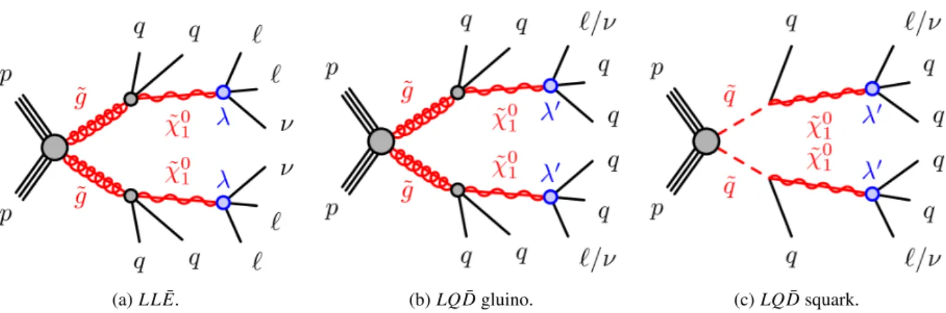
(a)LLE.¯ (b)LQD¯ gluino. (c)LQD¯ squark.

Figure 1: Diagrams illustrating theLLE¯andLQD¯ simplified models.

events and the ATLAS data. Signal cross-sections are calculated to next-to-leading order in the strong coupling constant, adding the resummation of soft gluon emission at next-to-leading-logarithmic accuracy (NLO+NLL) [56–60]. Both right- and left-handed squarks are taken into account in the squark produc- tion cross-section calculation. The nominal cross-section and the uncertainty are taken from an envelope of cross-section predictions using different PDF sets and factorisation and renormalisation scales, as de- scribed in Ref. [61].

The production and decay processes for the three simplified models are illustrated in Fig.1, which also introduces the names used for the three models: “LLE”, “LQ¯ D¯ gluino” and “LQD¯ squark”. These models are described further in the following.

3.1.1. LLE¯ model

In theLLE¯model, the ˜χ⁰₁LSP decays into two charged leptons and a neutrino. All possible combinations of charged leptons, including taus, are simulated in each sample; arbitrary branching fractions are tested by reweighting the events in each sample to match the desired hypothesis. The weight applied to each LSP decay is the ratio of the desired branching fraction and the simulated branching fraction for the appropriate decay mode, and the event weight is the product of the weights from both LSPs. To reduce the number of final states to a manageable number, no distinction is made between electrons and muons when this reweighting is performed – it has already been seen that the 4L search sensitivity is comparable in the two cases [27]. Thus, there are effectively three LSP decay modes: ``ν, `τν andττν, where` (without a subscript) refers to a light lepton. If a single LLE¯ coupling dominates, the allowed decay modes are fixed as follows (i,j,k ∈ {1,2}in the following):

λ_{i j k}: 100%``ν;

λi3k =−λ3ik: 50%``νand 50%`τν;

λ_{i j3}: 100%`τν;

λ_i33=−λ_3i3: 50%`τνand 50%ττν.

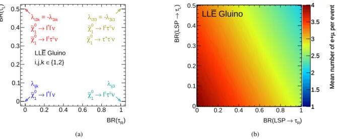
The interpretations in this document span the LSP decay space between these extremes, using two axes to differentiate between left-handed (Li/j) and right-handed ( ¯E_k) superfields, as shown in Fig.2a. At the

R) τ BR(

0 0.2 0.4 0.6 0.8 1

)LτBR(

0 0.1 0.2 0.3 0.4 0.5

λ3ik i3k = - λ

-ν

+l

→ l

0

χ∼1

ν±

±τ

→ l

0

χ∼1

λijk

ν l-

l+

→

0

χ∼1

λ3i3 i33 = - λ

ν±

±τ

→ l

0

χ∼1

ν τ-

τ+ 0→ χ∼1

λij3

ν±

±τ

→ l

0

χ∼1

Gluino E LL

{1,2}

∈ i,j,k

(a)

per eventµMean number of e+

1 1.5 2 2.5 3 3.5 4

per eventµMean number of e+

1 1.5 2 2.5 3 3.5 4

R) τ

→ BR(LSP

0 0.2 0.4 0.6 0.8 1

)Lτ→BR(LSP

0 0.1 0.2 0.3 0.4 0.5

Gluino E

LL

(b)

Figure 2: (a) Sketch of theLLE¯ coupling plane, showing the limiting cases of “pure” ˜χ⁰₁ decays at the corners.

(b) Mean number of light leptons per event, including those fromτ decays (35.2% leptonic branching fraction assumed).

origin, the LSP decays only to light leptons, ˜χ⁰₁ →``ν. Along thexaxis, the branching fraction to taus increases linearly until the LSP decays entirely to`τν. This corresponds to a transition from a regime whereLLE¯ couplings with first- and second-generation right-handed superfields dominate to one where the third generation dominates. The associated axis is marked BR(τ<sub>R</sub>). Along the y axis an analogous transition is made, this time involving the left-handed superfields, marked BR(τ<sub>L</sub>). As noted above, a maximum branching fraction of 50% to`τν is assumed in this case (for BR(τ_R) = 0), corresponding to a pure λ_i3k coupling withi,k , 3. Away from the x and y axes, a mixture of all nine possible LLE¯ couplings exists, with BR(τ_R) and BR(τ_L) assumed to be independent of each other. At every point in the plane, the sum BR(τ_L)+BR(τ_R) corresponds directly to the mean number of taus produced per LSP decay, which has a maximum value of 1.5 in the upper-right corner of the plane. Figure2b shows the mean number of light leptons per event, assuming two ˜χ⁰₁ decays and accounting for fully leptonic tau decays. By construction this is greatest at the origin, where there must be four light leptons per event, but even in the most extreme case there are more than two light leptons per event on average, which helps to provide good signal/background discrimination in this model.

The relative rates of the different LSP decay modes are related to the squares of the appropriate LLE¯ couplings, however the correct mapping of the RPV coupling values to the axes of Fig.2would need to be evaluated separately for any particular SUSY model. The reason is that the partial widths of each decay mode depend on the masses of virtual SUSY particles (in this case sleptons) that are not specified in the simplified model, and on the composition of the LSP. For the same reason, the lifetime of the LSP depends on the underlying RPV coupling values in a model-dependent way. However, for slepton and squark massesO(1 TeV), RPV coupling values of q

Pλ²_{i j k}+Pλ⁰_{i j k}² &10⁻⁴might reasonably be expected to yield a promptly decaying neutralino.

τ) BR(

0 0.1 0.2 0.3 0.4 0.5

BR(b)

0 0.2 0.4 0.6 0.8 1

' ij3

λ

±qb

→ l

0

χ∼1

ν qb

→

0

χ∼1

' ijk

λ

±qq'

→ l

0

χ∼1

ν qq'

0→ χ∼1

' 3j3

λ

±qb τ

→

0

χ∼1

ν qb

→

0

χ∼1

' 3jk

λ

±qq' τ

0→ χ∼1

ν qq'

0→ χ∼1

Squark D Gluino, LQ D

LQ {1,2}

∈ i,j,k

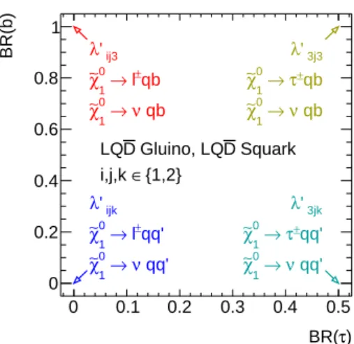
Figure 3: Sketch of theLQD¯ coupling plane, showing the limiting cases of “pure” ˜χ⁰₁decays at the corners.

3.1.2. LQD¯ models

In the twoLQD¯ models, the neutralino LSP decays into two quarks and a lepton. As withLLE¯couplings, the precise decay modes depend on whichλ⁰_{i j k} couplings are active. A specific non-zero couplingλ⁰_{i j k} allows the following decays:

χ˜⁰₁ →`_iu_jd_k and ˜χ⁰₁→ν_id_jd_k, (6) whereu and d denote up-type and down-type quarks, respectively. Equal branching fractions for the decay modes in Eq. (6) are assumed throughout.

As for theLLE¯ model, no distinction is made in this analysis between fermions of the first and second generations. A neutralino LSP can decay to third-generation fermions via any or all of the superfields involved in the LQD¯ superpotential term. Taus can be produced with λ⁰_{3j k} couplings, via left-handed slepton fields, with a maximum branching ratio of 50% (the other 50% produce tau neutrinos). Similarly, λ⁰_{i j3} couplings involve third-generation right-handed down-type squarks and allow decays withbquarks with branching ratios up to unity. Couplings with third-generation left-handed squarks (λ⁰_i3k) are more complicated due to the large top-quark mass affecting the relative rates of `tq vs νbq decays, which will not be discussed further here. Only the first two variations described will be considered. Again, a two-dimensional coupling plane is constructed, illustrated in Fig.3, with the branching ratio to taus and b-quarks as independent free parameters. In the same way as for the LLE¯ model, the LSP lifetime and the branching fractions used here relate to the underlyingλ⁰_{i j k}couplings in a model-dependent way.

3.1.3. Sparticle masses and kinematics

Each simulated sample is generated with a fixed ratioRbetween the LSP and NLSP masses, which take the values

R= m( ˜χ⁰₁)

m(NLSP) =0.1, 0.5 or 0.9. (7)

The 4L analysis has already demonstrated sensitivity to a wide range of ˜χ⁰₁masses (10 tom_NLSP−10 GeV) in the case ofLLE¯ decays. The sensitivity to promptLQD¯ decays has not previously been explored by

NLSP RPV decays m(NLSP) R

˜

g LLE¯ 800–1600 GeV 0.1

˜

g LLE¯ 1000–1600 GeV 0.5

˜

g LLE¯ 1000–1600 GeV 0.9

˜

g LQD¯ 600–1400 GeV 0.1

˜

g LQD¯ 800–1400 GeV 0.5

g˜ LQD¯ 800–1400 GeV 0.9

˜

q LQD¯ 600–1000 GeV 0.1

˜

q LQD¯ 600–1200 GeV 0.5

˜

q LQD¯ 800–1400 GeV 0.9

Table 7: Simulated signal samples for theLLE¯andLQD¯ simplified models. The samples are defined by the choice of NLSP ( ˜gor ˜q) and its mass, the mass ratioR=m( ˜χ⁰₁)/m(NLSP) and the RPV decay pattern of the ˜χ⁰₁. In every case, the NLSP mass is incremented by 200 GeV between samples.

any ATLAS search, except in the case of direct decays of third-generation squarks [22]. More details on the sparticle masses used in each model are given in Table7.

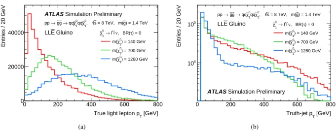
Fixing Rat particular values keeps the speed of the LSP in the rest frame of the NLSP approximately constant as the NLSP mass increases. Some consequences of this are shown in the kinematic distributions of Figs.4 and5, which are made for illustration without any detector simulation. The decay products of the LSP become softer and/or more collimated as Rdecreases, an effect which can be seen in both Figs.4aand5, where the relevant particles (charged leptons and neutrinos, respectively) arise only from the LSP decays. In contrast, the particles from the NLSP cascade decays become more energetic and well-separated. This is illustrated for jets in the LLE¯ model in Fig. 4b, which arise from the gluino decays and also the underlying event, which is the same in all three cases. Thus, the value ofReffectively determines how the available energy is shared between the final-state objects, and may affect the optimal choice of search strategy for a given model. In particular, the case of low values of R is expected to challenge existing analyses due to the reducedE_T^missfrom neutralino decays, and ultimately may require special techniques to detect [62].

3.2. Analysis strategy

Recalling Table1, it is expected that a variety of existing ATLAS analyses have the potential to be sensit- ive to theLLE¯ andLQD¯ simplified models described above. In the case of theLLE¯ model, there are four charged leptons in every event, and at least half of these are light leptons (see Fig.2b). Thus, we consider analyses that require high charged-lepton multiplicities, as the additional background rejection from this requirement allows looser requirements on other criteria such asE_T^miss. The 4L analysis was specifically designed withLLE¯ RPV decays in mind, and includes selections with hadronically decaying taus as well as light leptons. Here, for the first time, the SS/3L analysis is also considered. The requirement of a high jet multiplicity (see Table3) is easily fulfilled for the gluino model considered here, while the lower lepton multiplicity requirement leads to gains in the signal efficiency with respect to the 4L analysis.

All of the search channels in Table1requiring zero or one light lepton are potentially sensitive to one or more of theLQD¯ models, although the analysis sensitivity is expected to be reduced with respect to RPC SUSY models, as the only source of E_T^miss is from neutrinos produced in decays of the ˜χ⁰₁ LSP.

[GeV]

True light lepton pT

0 200 400 600 800

Entries / 20 GeV

0 20000

40000 ⁰→ l⁺l^-ν, BR(τ) = 0 χ∼1

) = 140 GeV

0

χ∼1

m(

) = 700 GeV

0

χ∼1

m(

) = 1260 GeV

0

χ∼1

m(

ATLAS Simulation Preliminary

) = 1.4 TeV g~ = 8 TeV, m(

s

0, χ∼1 0qq χ∼1

→ qq g~ g~

→ pp

Gluino E LL

(a)

[GeV]

Truth-jet pT

0 200 400 600 800

Entries / 20 GeV

104

105 ⁰→ l⁺l^-ν, BR(τ^{) = 0}

χ∼1

) = 140 GeV

0

χ∼1

m(

) = 700 GeV

0

χ∼1

m(

) = 1260 GeV

0

χ∼1

m(

ATLAS Simulation Preliminary

) = 1.4 TeV g~ = 8 TeV, m(

s

0, χ∼1 0qq χ∼1

→ qq

~g g~

→ pp

Gluino E LL

(b)

Figure 4: (a) Light-lepton p_T distributions and (b) jetp_T distributions for three different ˜χ⁰₁ masses in the LLE¯ model withm( ˜g) =1.4 TeV. All light leptons withp_T >10 GeV and|η|<2.5 are shown, while jets are required to havep_T>20 GeV and|η|<4.5.

[GeV]

miss

True ET

0 200 400 600 800

Entries / 20 GeV

0 5000 10000 15000

BR(b) = 0 ) = 0.5 τ qq, BR(

ν

→ l/

0

χ∼1

) = 100 GeV

0

χ∼1

m(

) = 500 GeV

0

χ∼1

m(

) = 900 GeV

0

χ∼1

m(

) = 1.0 TeV g~ = 8 TeV, m(

s

0, χ∼1 0qq χ∼1

→ qq g~ g~

→ pp

ATLAS Simulation Preliminary

Gluino D LQ

Figure 5:E_T^missdistributions for three different ˜χ⁰

1masses in theLQD¯ gluino model withm( ˜g)=1.0 TeV.

While in principle events with two light leptons are also produced, the SS/3L analysis is found to be insensitive, due to the lack of hard neutrinos from the ˜χ⁰₁ decays in this case. The 0L 7–10 jets search is only considered for the model with gluino pair production, as too few jets are produced in the squark model to satisfy the selection criteria.

In all three models, the method for setting the best limit on SUSY production is the same. Each point in the parameter space is fully described by the model type, the LSP/NLSP mass ratio R, the NLSP massm_{g/˜ q˜}, and the (x,y) position in the coupling plane. At each of these points, each channel uses its own selection and statistical analysis procedure to set a 95% confidence level (CL) exclusion limit on the signal strength, µ_lim. By convention, limits are set with respect to the theoretical signal cross- section reduced by one standard deviation, and µ_lim = 1 corresponds exactly to exclusion of this cross- section. The expectedµ_limvalue, assuming no signal in the data, is also calculated at each point by each channel. Channels within a single search are statistically combined where possible, as described in the corresponding analysis papers.2 Channels from different searches are not combined, and sometimes it is also not possible to combine channels within a single search. Where multiple sensitive channels cannot be combined, the channel with the best expected limit is chosen to constrain each point in the parameter space. The corresponding observedµ_limvalues are used directly to extract limits on the production cross- section at each point (with results in Apps.A,BandC). Lower bounds on the NLSP mass are obtained by linear interpolation of ln(µ_lim) between points with different NLSP masses. The limit is placed at the mass whereµ_lim=1.

Experimental systematic uncertainties on the signal modelling are estimated using the procedures de- scribed within each analysis paper. Model-dependent theoretical uncertainties on the analysis acceptance are also accounted for. These are calculated by varying the renormalisation and factorisation scales, as well as the amount of initial- and final-state radiation. Events are generated for each variation using MadGraph5 v1.5.12 [63], with showering performed by Pythia6.427 [64]. No detector simulation is performed; instead, kinematic selections are applied to the generated particles, as described in Ref. [65].

For the 4L and SS/3L analyses, the corresponding uncertainties are of order a few percent, and small compared to other sources of uncertainty. In the 1L search these uncertainties are neglected as they are estimated to be negligible. For the 0L 2–6 jets and 0L 7–10 jets analyses, these uncertainties can reach as high as∼30% forR=0.1, with a statistical precision of about 5%. Compared to the other searches, these two analyses use higher jet p_T thresholds, and are therefore more reliant on QCD radiation in order to satisfy the SR selection criteria. In such cases, this is often the dominant source of systematic uncertainty on the model’s acceptance.

As described in Sect.2, it is important to also consider the potential contamination of signal events in control and validation regions used by these searches. Upon examination, it is found that the contamina- tion is almost always significant only for low squark and gluino masses that are very well excluded (often by more than one search). For example, there is significant contamination in the SS/3L validation regions in theLLE¯ model withm( ˜g) = 800 GeV andR = 0.1, but this scenario has already been conclusively ruled out by the 4L search [27]. Similarly, the contamination of CRW in the 0L 2–6 jets search can reach as high as 55% of the observed events in data for theLQD¯ gluino model withm( ˜g) =1.0 TeV, but when the 1L results are taken into account this too is far from the observed mass limit. The main exception to this trend occurs for CRQ in the 0L 2–6 jets analysis and in the control regions used to control thet¯t andW+jets backgrounds in the 0L 7–10 jets analysis. In both cases, the SUSY signal can saturate the observed data in the control regions. For the 0L 2–6 jets analysis, this is important only when the LSP

2For the purposes of this discussion, a “search” corresponds to a single row of Table1.

is relatively light (R = 0.1), while for the 0L 7–10 jets analysis it is important for m( ˜g) . 1 TeV. In both cases, the control region contamination is taken into account when setting limits, which can weaken them relative to hypothetical scenarios where this effect could be neglected. This indicates that to fully optimise these searches for RPV SUSY scenarios, alternative background estimation techniques would need to be explored.

3.3. Results

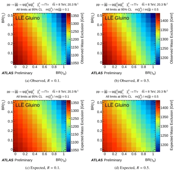
The lower limits on the gluino mass for the LLE¯ simplified models are shown in Figs. 6 and 7, for the three values ofRthat are considered. The observed and expected limits are evaluated based on the nominal signal cross-section reduced by its 1σ theoretical uncertainty. For R = 0.1 and 0.5, the best constraints come from the SS/3L search. The 4L analysis provides weaker constraints, despite targeting RPV SUSY, as it was not optimised explicitly for squark and gluino production. In the SS/3L analysis, different signal regions are statistically combined, however the constraints are driven by the SR3Lhigh signal region defined in Table 3. This region requires at least three light leptons, and as a result the strongest constraints are set when the LSP decays entirely to light leptons in the lower left corner of the plane. Comparing with Fig.2, it can be seen that the limits weaken as the average number of light leptons per event decreases. In the case of R = 0.9, the jets from the gluino decays are less energetic and the 4L analysis can constrain the model more strongly in the region indicated in Fig.7c, where the average light lepton multiplicity is greater than approximately 3.4. The constraint in this case is dominated by the SR0noZb region, which requires at least four light leptons, and the signal regions with taus do not contribute significantly to the final results. Overall, the strongest constraints are obtained for R = 0.5 where the available energy can be distributed more or less evenly between all of the leptons and jets, and the weakest constraints for tau-rich scenarios are obtained forR =0.1 where the light leptons from leptonic tau decays are more likely to be soft or collimated with other leptons.

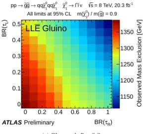
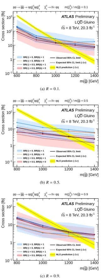
A selection of upper cross-section limits for the LLE¯ model are shown in Fig.8, corresponding to the pure LLE¯ couplings at the four corners of the coupling plane, for which explicit decay patterns were given in Fig.2a. The observed and expected limits show a strong dependence on the average light lepton multiplicity in the LSP decays. By comparison, the dependence of the limits on the gluino mass is relatively weak. The complete set of upper limits on the production cross-section for this model and more details on which analysis results are used at each point in the parameter space are given in App.A.

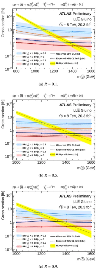
Corresponding lower limits on the gluino mass for the LQD¯ gluino model are shown in Figs.9and10.

The signal model nominally produces eight jets (in addition to jets from hadronically decaying taus), and for R = 0.1 and 0.5 the 0L 7–10 jets analysis produces the strongest constraints. The statistical combination of signal regions requiring ab-jet and those with ab-jet veto (see Table5) leads to a non- trivial dependence on BR(b), with values of 0 and 1 being preferred. The limits also have a strong dependence on BR(τ), as a veto on light leptons is applied. As for theLLE¯ model, the mass limits are weaker forR=0.1 than R=0.5, with the higherp_Tthresholds for jets compared to leptons significantly amplifying the observed effect. For R = 0.9 the SUSY spectrum is compressed and the 0L 7–10 jets analysis no longer produces the best results, as it is highly dependent on reconstructing the jets from the gluino cascade. The 1L and 0L 2–6 jets analyses set powerful constraints in the regions BR(τ) ≤ 0.1 and≥0.3, respectively. The final expected limits depend only weakly upon BR(τ) and BR(b), due to the excellent complementarity between the two searches.

Observed Mass Exclusion [GeV]

1050 1100 1150 1200 1250 1300 1350

R) τ BR(

0 0.2 0.4 0.6 0.8 1

)LτBR(

0 0.1 0.2 0.3 0.4 0.5

ATLAS Preliminary

= 8 TeV, 20.3 fb-1

s ν l-

l+

→

0

χ∼1 0 χ∼1 0qq χ∼1

→ qq g~ g~

→ pp

) = 0.1

~g ) / m(

0

χ∼1

All limits at 95% CL m(

Gluino E

LL

(a) Observed,R=0.1.

Observed Mass Exclusion [GeV]

1200 1250 1300 1350 1400

R) τ BR(

0 0.2 0.4 0.6 0.8 1

)LτBR(

0 0.1 0.2 0.3 0.4 0.5

ATLAS Preliminary

= 8 TeV, 20.3 fb-1

s ν l-

l+

→

0

χ∼1 0 χ∼1 0qq χ∼1

→ qq g~ g~

→ pp

) = 0.5 g~ ) / m(

0

χ∼1

All limits at 95% CL m(

Gluino E

LL

(b) Observed,R=0.5.

Expected Mass Exclusion [GeV]

1050 1100 1150 1200 1250 1300 1350

R) τ BR(

0 0.2 0.4 0.6 0.8 1

)LτBR(

0 0.1 0.2 0.3 0.4 0.5

ATLAS Preliminary

= 8 TeV, 20.3 fb-1

s ν l-

l+

→

0

χ∼1 0 χ∼1 0qq χ∼1

→ qq g~ g~

→ pp

) = 0.1

~g ) / m(

0

χ∼1

All limits at 95% CL m(

Gluino E

LL

(c) Expected,R=0.1.

Expected Mass Exclusion [GeV]

1200 1250 1300 1350 1400

R) τ BR(

0 0.2 0.4 0.6 0.8 1

)LτBR(

0 0.1 0.2 0.3 0.4 0.5

ATLAS Preliminary

= 8 TeV, 20.3 fb-1

s ν l-

l+

→

0

χ∼1 0 χ∼1 0qq χ∼1

→ qq g~ g~

→ pp

) = 0.5 g~ ) / m(

0

χ∼1

All limits at 95% CL m(

Gluino E

LL

(d) Expected,R=0.5.

Figure 6: Observed and expected 95% lower limits on the gluino mass for theLLE¯simplified model withR=0.1 and 0.5. These limits are obtained using the SS/3L search results.