Non-discriminatory Trade Policies in Structural Gravity Models. Evidence from Monte Carlo Simulations

IHS Economics Series Working Paper 335

November 2017

Non-discriminatory Trade Policies in Structural Gravity Models. Evidence from Monte Carlo Simulations

Richard Sellner

Impressum Author(s):

Richard Sellner Title:

Non-discriminatory Trade Policies in Structural Gravity Models. Evidence from Monte Carlo Simulations

ISSN: 1605-7996

2017 Institut für Höhere Studien - Institute for Advanced Studies (IHS) Josefstädter Straße 39, A-1080 Wien

E-Mail: o ce@ihs.ac.atffi Web: ww w .ihs.ac. a t

All IHS Working Papers are available online: http://irihs. ihs. ac.at/view/ihs_series/

This paper is available for download without charge at:

https://irihs.ihs.ac.at/id/eprint/4467/

Non-discriminatory Trade Policies in Structural Gravity Models

Evidence from Monte Carlo Simulations

Richard Sellner¹

1Institute for Advanced Studies (IHS), Josefst¨adter Straße 39, AT-1080 Vienna

November 21, 2017

Abstract

This paper provides Monte Carlo simulation evidence on the performance of methods used for identifying the effects of non-discriminatory trade policy (NDTP) variables in structural gravity models (SGM). The benchmarked methods include the identification strategy of Heid, Larch & Yotov (2015) that utilizes data on intra-national trade flows and three other methods that do not rely on this data. Results indicate that under the assumption of a data generating process that conforms with SGM theory, data on intra-national trade flows is required for identification. The bias of the three methods that do not utilize this data, is a result of the correlation between the NDTP variable and the collinear fixed effects. The MC results and an empirical application demonstrate the severity of this bias in methods that have been applied in previous empirical research.

Keywords Structural Gravity Model, Non-discriminatory Trade Policies, Monte Carlo Simulation.

JEL Classification C31, F10, F13.

1 Introduction

Estimating the effects of trade policy variables on trade flows is a major interests in international eco- nomics. Since the seminal paper of Anderson & van Wincoop (2003), there has been a substantial amount of empirical research involving the econometric estimation of these effects within a structural gravity framework, noting the importance of theory-consistent treatment of the multilateral resistance terms (MRT) to obtain unbiased estimates. Most of the empirical applications on the structural gravity model focused on the estimation of the effects of discriminatory trade policy measures, among them very prominently regional trade agreements (see Anderson & Yotov, 2016; Bergstrand, Larch & Yotov, 2015;

Egger, Francois, Manchin & Nelson, 2015, for recent contributions). Estimation is mostly done via Poisson Pseudo-Maximum Likelihood (PPML), including importer and exporter fixed effects in a cross-sectional, and importer-time, exporter-time fixed effects in a panel setting, to control for the MR-terms.

This identification strategy will, however, fail if the variable of interest lacks variation in both im- porter and exporter (i.e. importer-time and exporter-time) dimension, since it will be perfectly collinear to one of the fixed effects. As Head & Mayer (2014) mentioned, such variables will include anything that affects a country’s propensity to export/import to/from all destinations or sums, averages and dif- ferences of country-specific variables. Among those, economists are especially interested in the effects of non-discriminatory trade policy (NDTP) measures on trade flows and subsequent welfare effects. NDTP measures include most-favored nation tariffs (see Piermartini & Yotov, 2016), export subsidies or pro- motion (see Lederman, Olarreaga & Payton, 2010) and trade facilitation (see Hoekman & Nicita, 2011;

Beverelli, Neumueller & Teh, 2015), among others.

Estimation of NDTP in structural gravity models has only recently been addressed more thoroughly in the literature. Head & Mayer (2014) devoted a subsection in their summary contribution of the gravity model to this topic and Piermartini & Yotov (2016) mentioned the identification problems of the effects on those variables as one of the challenges in empirical structural gravity estimation. Piermartini & Yotov (2016) referred to a method recently introduced in Heid et al. (2015), where the authors suggest to use data on intra-national trade flows to identify the effects of NDTP. Contrary to the MRT captured by the fixed effects, the NDTP measures should not affect intra-national trade, introducing bilateral variation.

While this identification method is consistent with structural gravity theory and seems very promising, it requires data on domestic trade, i.e. goods and services that are nationally produced and consumed.

Since data on such flows is often not readily available or reported with a substantial time lag, researchers have often resorted to different methods to obtain estimates on their NDTP measures of interest.

In cases where data on intra-national trade flows is unavailable, Head & Mayer (2014) and Piermartini

& Yotov (2016) suggested to use a two-stage fixed effects identification strategy, in which the fixed effects, obtained from the first stage, are regressed onto the NDTP measure and other country-specific variables. This approach has been frequently applied in empirical research to identify the effects of

collinear variables (see for instance Eaton & Kortum, 2002; Melitz, 2008; Head & Ries, 2008; Anderson

& Yotov, 2016). Another popular method (see for instance Portugal-Perez & Wilson, 2012; Bratt, 2017) is the ’Bonus-Vetus OLS’ introduced by Baier & Bergstrand (2009). Here, the MRT are approximated by the doubly-demeaned trade cost variables, thus avoiding the collinearity problem. Recently, Prehn, Brmmer & Glauben (2016) motivated the use of a random intercept PPML estimator to identify country- specific variables in the presence of collinearity. They demonstrated the performance on the US-Canadian dataset used in Anderson & van Wincoop (2003) and reported estimates for distance and border similar to a PPML FE estimator, while also being able to obtain estimates on the exporting and importing countries GDP elasticities.

Despite the increasing interest and discussion surrounding NDTP in structural gravity models, little is known about the properties of the proposed estimators. In general, there exist only a few Monte Carlo studies that explicitly take into account a data generating process (DGP) that is consistent with structural gravity theory (see for instance Baier & Bergstrand, 2009; Head & Mayer, 2014; Egger &

Staub, 2016). Since none of these studies focused on NDTP measures, this paper aims at closing this gap.

The benchmarked methods include (1) fixed effects estimation on intra-national data, (2) Bonus-Vetus, (3) two-stage fixed effects and (4) random intercept PPML. The latter three are estimated assuming data on intra-national trade flows is not available, the case in which these methods are usually used in empirical research. The paper contributes to the existing literature by analysing the properties of these estimators proposed in the literature in Monte Carlo experiments based on a DGP that is consistent with an economic motivation of the structural gravity model. As most of the current empirical studies implement the estimation via PPML, a DGP based on a generalized linear model (GLM) framework will be employed. The results will be particularly interesting for empirical researchers that have in the past employed one of the methods or are aiming at identifying the effects of NDTP under a structural gravity model in upcoming research.

The main finding is that, given a DGP that conforms with structural gravity theory, data on intra- national trade flows is needed for identification. The bias of the methods that do not employ this data relates to the correlation of the NDTP variable of interest with the corresponding collinear fixed effects.

The three methods disregarding intra-national observations for identification only yield unbiased estimates in a scenario in which this correlation is explicitly set to zero. An illustrative empirical application confirms the direction of the bias that is to be expected if these methods are used.

The remainder of the paper is organized as follows. The next section gives a short introduction to the structural gravity model and discusses the methods that are benchmarked in the Monte Carlo experiments. Section 3 describes the Monte Carlo simulation design, outlines the scenarios analysed and closes with the results. Section 4 demonstrates the methods on an empirical application. A final section concludes.

2 Non-discriminatory Trade Policies in Gravity Models

2.1 Structural Gravity Model

As in Egger & Staub (2016), the structural gravity model is motivated on grounds of an endowment economy with Armington differentiation. To avoid cluttered notation and reduce the computational effort in the MC simulations, the analysis will focus on a cross-section of aggregate bilateral trade flows between countries for a given period.¹ Each country i= 1, . . . N is endowed with a volume of goodsHi

that it sells at a mill price pi to earn incomeYi =piHi. As Anderson & van Wincoop (2003) showed, the import demand of countryj for goods ofisatisfies²

X_ij = p^α_iτ_ij^αYj

PN

k=1p^α_kτ_kj^α, (1)

whereτij ≥1 are the iceberg trade costs and 1−αis the elasticity of substitution (withα <0) under this model.³ Imposing the market-clearing conditionPN

j X_ij =Y_i to Eq. (1) and solving for the equilibrium market price yields

p^1−α_i = 1 H_i

N

X

j=1

τ_ij^αp_jH_j PN

k=1p^α_kτ_kj^α, (2)

which implicitly determinespiandYi, givenαand the joint distribution ofτijandHi(see Egger & Staub, 2016). Substituting this price back into the import demand equation and definingP_j^α=PN

i=1(piτij)^αas the CES price index results in the well-known structural gravity model

X_ij = Y_iY_j τ_ij

ΠiPj

α

, (3)

Π^α_i =

N

X

k=1

τik

P_k ^α

Y_k, (4)

P_j^α =

N

X

k=1

τkj

Π_k ^α

Yk, (5)

withYi andYj being production and expenditures, whereas for simplicity balanced trade is assumed.

From the definition of the multilateral resistance terms (MRT) given in Eq. (4) and (5) it follows, that E[Πiτij]6= 0,E[Pjτij]6= 0 andE[ΠiPj]6= 0. Addressing this correlation structure will be a central feature of the DGP that will be used for the Monte Carlo simulations. To be consistent with a structural

1Note that most of the current research employs panel data sets and/or covers specific sectors or product groups.

Exploiting the time variation via a panel data structure is strongly recommended in Piermartini & Yotov (2016), whereas they suggest to include every third or fifth year to permit adjustment of trade flows to policy changes. However, note that for the questions addressed in this paper, a cross-section setting will suffice.

2For simplicity, the exporter-specific preference parameter from the original specification of Anderson & van Wincoop (2003) is omitted.

3Various types of models motivated from the demand or supply side suggested in the literature yield a model of the type presented here (see for example Anderson & van Wincoop, 2003; Eaton & Kortum, 2002; Melitz, 2003; Chaney, 2008).

These models only differ in their interpretation of the elasticity of trade flows with respect to trade costsα.

gravity model, pricespineed to be determined endogenously from the structure of the model. Production and expenditure in turn depend on the prices and, along with the trade costs, determine the trade flows.

Eqs. (1) and (2) can therefore be used to generate the endogenous variables pi, Yi and the structural part⁴of the trade flows, consistent with the economic structure of the model.

2.2 Econometric Specification

Specifying the unobserved trade costsτ_ij^αand introducing a stochastic term, the model given by Eqs. (3) - (5) can be re-written in a form that can be econometrically estimated. Denotingei= ln (Yi/Π^α_i),mj= ln Yj/P_j^α

and specifying the trade costs by a vector of observable variablesβDij+γN IPij = ln τ_ij^α , leads to

X_ij = exp (e_i+m_j+βD_ij+γN IP_ij)η_ij. (6) To keep the model simple, only one discriminatory trade cost variable D_ij and one non-discriminatory import protection measure N IPij is assumed. A non-discriminatory trade policy, per definition, affects all trading partners equally, but will not exert an impact on goods and services that are domestically produced and consumed(see Heid et al., 2015), i.e. Xii. Thus,N IPij=N IPj ∀ i6=jandN IPjj = 0.

The assumptions about the multiplicative errorηij will determine which model will be identified. For instance, OLS on a log-linearized version of Eq. (6) will be identified ifE(lnηij|ei, mj, Dij, N IPij) = 0, i.e. there is no dependence between the covariates and the logarithm of the error term. Assuming E(η_ij|ei, m_j, D_ij, N IP_ij) = 1, i.e. the errors are mean-independent of the covariates, permits identifica- tion via a GLM estimator.⁵ Santos Silva & Tenreyro (2006) showed that the errors in gravity models of trade will in general be heteroscedastic and dependent on the covariates. OLS estimation on a log-linear version of Eq. (6) will then yield biased estimates due to Jensen’s inequality. Furthermore, the presence of zero flows will provoke ad hoc solutions in log-linear models. Since the bulk of the current empirical gravity models are estimated in multiplicative form, mostly by PPML following the arguments brought in Santos Silva & Tenreyro (2006), the focus of this paper will be on GLM estimation with a log-link function and a Poisson family. GLM estimates will be consistent if the conditional mean function is cor- rectly specified. The efficiency of the estimator will depend on correct specification of the error variance, i.e. the linear exponential family of the density chosen.

There are three different approaches towards a theory-consistent estimation of Eq. (6) that controls for the structure imposed bye_i andm_j. The most common procedure is to includeN−1 exporter and N−1 importer fixed effects fore_iandm_j(see Harrigan, 1996; Feenstra, 2004). A second option is to apply

4The structural part can be obtained by assuming that Eq. (1) only holds in expectation, replacingXijbyE(Xij).

5Recently, Figueiredo, Lima & Orefice (2016) argued that if one assumes that the log-linear model is identified, then the GLM estimates will be severely biased. Since the researcher cannot know which model is true, they proposed a robust quantile estimation approach.

a structurally-iterated estimator (Head & Mayer, 2014; Egger & Staub, 2016). Given a set of starting values foreiandmj, Eq. (6) is estimated via GLM, restricting the coefficients oneiandmj to one. The results are used to obtain an estimate of τ_ij^α, which is employed to solve for new estimates ofei andmj. This procedure is repeated until convergence. A third option is the quasi-differences estimation, that uses two products of country-pairs to net oute_i andm_j. This can be done either by using just-identified set of moment conditions (as described in Charbonneau, 2012) or apply a simply ratio-of-ratios estimator as outlined in Head & Mayer (2014) or Egger & Staub (2016). The latter can be implemented by GLM estimation on the sets of transformed variables Xs =XikXlj/XlkXij and ds = (dik+dlj)−(dlk+dij) withdbeing a trade cost variable.⁶

2.3 Identification via intra-national trade flows

Given the conditional mean is correctly specified, fixed effects, structurally-iterated and quasi-differences estimation will yield consistent estimates for bilaterally varying trade cost variables. If data on intra- national trade flows is available, these methods may also be applied to identify the effects of non- discriminatory trade policies in a structural gravity model. This identification strategy has just re- cently been introduced by Heid et al. (2015) and the approach is further discussed in Piermartini &

Yotov (2016). As Piermartini & Yotov (2016) mention, the intra-national dimension turns the monadic non-discriminatory trade policy variables into dyadic variables. The key identifying assumption is that non-discriminatory trade policies do not affect intra-national trade. Heid et al. (2015) suggested a fixed effects panel model that can be formulated as follows for a cross-sectional setting:

X_ij = exp λ^{F E}_i +χ^{F E}_j +β^{F E}D_ij+γ^{F E}N IP_ij

η_ij^{F E}. (7)

The unobserved terms ei and mj are captured by the fixed effects λ^{F E}_i and χ^{F E}_j . Identification is possible since the MRT will be identified over all country-pairs, including intra-national trade, while the non-discriminatory trade policies can be identified by exploiting the variation between intra-national and international flows.

Note that Eq. (7) may also be estimated via the structurally-iterated and the quasi-differences approach outlined above. However, the fixed effects estimator has several advantages. In contrast to the structurally-iterated estimator, the FE estimator imposes no specific structural assumptions on the MRT. The fixed effects will capture the MRT even if some key variables in determining the trade costs are omitted or unobserved. Furthermore, the structurally-iterated estimator is more prone to convergence failures than the fixed effects estimator (see Egger & Staub, 2016). Compared to the quasi-differences approach, the fixed effects estimator is computationally less demanding and leads to lower standard errors

6Giveni 6= land j 6=k there are numerous sets making estimation computationally demanding. To speed up the computation, the estimation may be performed on only a subset of all possible combinations, leading to efficiency losses.

(see Egger & Staub, 2016).

The main disadvantage of the FE estimator is that, while the coefficients are consistently estimated, the asymptotic variance might be affected by the incidental parameter problem. Cameron & Trivedi (2005) showed that in a multiplicative model with one-way fixed effects, the incidental parameter problem can be avoided by using a concentrated likelihood function. Still, in the case of a two-way fixed effect model such as Eq. (7) the problem remains. Egger & Staub (2016) showed in their Monte Carlo simulations that the incidental parameter problem strongly affects the t-statistics on their trade cost measure. As a solution to the problem Jochmans (2017) recently derived a GMM estimator for two-way multiplicative gravity models. As the focus of this paper is on the bias and consistency of the NDTP estimates, this is demonstrated in the MC simulations via the simpler fixed effects estimator.

2.4 Identification methods without intra-national trade flows

While there is ongoing interest in the effects of non-discriminatory and unilateral trade policies, the literature just recently started discussing the issue of their identification in structural gravity models. A challenge for empirical estimation occurs if data on intra-national flows is not available. This may be the case because they are not published for the countries of interest, or they are reported with a severe time lag and do not match the periods for which the data on non-discriminatory trade policies is reported.

Since in such a case the non-discriminatory trade policy measures will not vary over either the exporter or importer dimension, they will be perfectly collinear to one of the fixed effects and cannot be identified.

Furthermore, the collinearity will lead to convergence failure in the structurally-iterated estimates, since m_j andN IP_ij cannot be jointly identified. The quasi-differences procedure is also not applicable, since d_ik+d_lj=d_lk+d_ij and thusd_s= 0 for alls, thus none of the three methods discussed above will work.

One way to avoid collinearity is to simply construct a new dyadic variable from two monadic variables, taking into account that the functional form avoids collinearity. Examples from the literature include Lee

& Park (2007) or Mo¨ıs´e, Orliac & Minor (2011) that analysed the effects of trade facilitation indicators.

However, as Head & Mayer (2014) note, most of the dyadic indicators constructed this way may not have a straightforward interpretation. Another ad hoc solution to the problem, noted in Piermartini &

Yotov (2016), is to approximate the MRT by remoteness indexes, which has been the common practice in papers prior to Eaton & Kortum (2002) and Anderson & van Wincoop (2003). Head & Mayer (2014) discussed various frequently used remoteness measures and found that none of them can capture the structure imposed by the theory. In a similar manner Piermartini & Yotov (2016) do not recommend the use of such remoteness measures to substitute MRT or fixed effects.

As a more promising solution to the problem, Piermartini & Yotov (2016) and Head & Mayer (2014) propose a two-stage fixed effects procedure. First the coefficients on the bilaterally-varying trade cost variables are estimated along with exporter and importer fixed effects. Then the respective fixed effects of

the first stage are regressed on the NDTP and other country-specific variables. This two-step procedure has been frequently used in the literature. For instance, Eaton & Kortum (2001, 2002) used this set-up to identify key parameters of their trade models, Melitz (2008) estimated the effects of the literacy rate and a measure of linguistic diversity on trade, and Gylfason, Mart´ınez-Zarzoso & Wijkman (2015) adapted this procedure on a panel with time-varying non-bilateral data on corruption and democracy. Given its frequent use, this estimator will be included in the Monte Carlo simulations. Both stages will be estimated via GLM:

Xij = exp λ^2S_i +χ^2S_j +β^2SDij

η^2S_ij (8)

exp ˆχ^2S_j

= exp ψ^2S+δ^2SlnY_j+γ^2SN IP_j

ν_j^2S. (9)

The flaws of this procedure for obtaining an estimate of γ^2S under fixed effects assumption have been thoroughly outlined in the discussion that followed the fixed effects vector decomposition (FEVD) model introduced in Pl¨umper & Troeger (2007). As Greene (2011) noted, it is not possible to identify the fixed effects and collinear variables under the assumptions of a fixed effects model. Only the preceding linear mixture of the two is estimable. The parameter γ^2S is only separately identified if the fixed effects assumptionE(N IPjmj)6= 0 is violated. Another related approach to identify collinear variables was given in Egger (2005), who extended the Hausman & Taylor (1981) model (HTM) to the gravity framework. Besides being a log-linear model, the HTM imposes strong exogeneity assumptions on the discriminatory variables used as instruments for the identification of the effects of the NDTP measures.⁷ Another commonly applied approach to avoid the collinearity problem is the ’Bonus Vetus’ (BV) method (see Baier & Bergstrand, 2009), that approximates the multilateral resistance terms by a first- order log-linear Taylor series expansion around a symmetric trade cost world. To implement this method, compute x^{M RS}_ij = xij −M RS(xij) for each trade cost variable x, with M RS(xij) = PN

k=1xkjθk + PN

l=1xilθl−PN k=1

PN

l=1xklθkθl andθi=Yi/PN

k=1Yk. The normalized trade flowsXij/(YiYj) are then regressed on the transformed variablesx^{M RS}_ij . A more robust version for estimation purposes is to replace the GDP-weights with equal weights 1/N (see Baier & Bergstrand, 2010), which assumes a symmetric world in trade costs and economic sizes. While the BV method was originally derived for OLS on log-linearized model of Eq. (6), BV-transformed variables haven often been used in PPML estimation (see Hoekman & Nicita, 2011; Mo¨ıs´e & Sorescu, 2013; Bratt, 2017). Given its continuing popularity in empirical applications, the BV method (in its more robust, equally-weighted specification) is included in the Monte Carlo simulations:

7Note that assuming a log-linear model and that all bilateral variables are exogenous, the HTM will yield estimates similar to the second-stage of the FEVD and the tow-stage FE model.

Xij/(YiYj) = exp ψ^BV +β^BVD^{M RS}_ij +γ^BVN IP_ij^{M RS}

η_ij^BV (10)

As for all the methods in this section, it will be assumed that data on intra-national trade flows is un- available. However, data on intra-national observations for discriminating trade costs or NDTP variables is usually observed or in the case of NDTP they are per definition zero. The BV-transformation of the regressors can therefore be applied utilizing the information on the complete dataset ofN²observations, dropping the transformed intra-national observations prior to estimation. Note that in empirical research so far, the BV transformation is often applied only to discriminatory trade cost variables while NDTP variables are included as observed (see for instance Hoekman & Nicita, 2011; Mo¨ıs´e & Sorescu, 2013).

However, it can be shown by MC simulations that such an approach will result in biased estimates even under the most favourable assumptions concerning the DGP.⁸

In cases of no missing data and assuming a log-linear model with homoscedastic errors, Head &

Mayer (2014) showed in Monte Carlo simulations that the BV-method yields unbiased estimates for discriminatory trade policy variables. It can also be demonstrated that under these conditions the BV method on data including intra-national trade flows also yields unbiased estimates on the NDTP variable.⁹ Nevertheless, the use of the BV method is often motivated on grounds of collinearity in cases where data on intra-national flows is missing. It is therefore illustrative to assess the performance of the BV method in a GLM estimation framework without data on intra-national trade flows.

Estimates of such a model are subject to several sources of bias. First, under a multiplicative non-linear model with heteroscedastic errors, the log-linearized BV-transformations will lead to biased estimates, as shown in Santos Silva & Tenreyro (2006). Since the BV method resembles a double-demeaning procedure, their GLM counterpart would invoke concentrating out the mean effects of exporters and importers or applying some quasi-differences approach as described above. Such a procedure would strongly complicate the use of this method, whose popularity is a result of its simplicity for application. A second source of bias comes from missing observations, a problem that is usually encountered in empirical applications of the gravity model. As the MC results of Head & Mayer (2014) showed, this bias will be negligible for discriminatory continuous variables. A third source of bias can be attributed to the correlation between unobserved effects and the NDTP variable, which will be demonstrated later in this paper.

The last method that will be included in the Monte Carlo simulation is the random intercept PPML, recently proposed by Prehn et al. (2016) for the use in gravity models. They applied this estimator to the Anderson & van Wincoop (2003) data set and reported estimates on the distance and border coefficients, that are virtually identical to those obtained via fixed effect PPML. Additionally, they are able to estimate the coefficients on the countries incomes Y_i and Y_j and claim that this method allows

8See Table (5) and the accompanying text in the Appendix.

9See Table (5) in the Appendix.

to analyze policy-relevant importer or exporter-specific variables such as tariffs and infrastructure. The random intercept PPML can be written as:

X_ij = exp λ^RI_i +χ^RI_j +β^RID_ij+γ^RIN IP_ij

η_ij^RI, (11)

λ^RI_0i ∼ N(0, σ²_λ0i), (12)

χ^RI_0j ∼ N(0, σ²_χ

0j), (13)

with priors λ^RI_0i and χ^RI_0j on the importer and exporter effects.¹⁰ Identification of the NDTP variable within this model is possible because the individual exporter and importer effects are modelled via random effects. In large samples the effect of the prior will vanish and the Laplace approximation employed in the estimation algorithm used in Prehn et al. (2016) will push the posterior mode towards the maximum- likelihood estimator of the fixed effects model. Therefore the estimates on their discriminatory trade policy variables are identical to the fixed effects PPML. If the random intercepts tend to coincide with the fixed effects, one would expect the collinear country-specific variables to be identified in similar manner than in the two-stage FE approach. Thus, if these variables are correlated with the unit effects, biased estimates are expected. As in Prehn et al. (2016), theglmer function of the R-packagelme4 (see Bates, M¨achler, Bolker & Walker, 2015) with random intercepts and a Poisson family will be used in the MC simulations.

For comparison to the above models, a naive gravity model is added to the MC simulations:

Xij = exp ψ^naive+β^naiveDij+γ^naiveN IPij+ω1lnYi+ω2lnYj

η_ij^naive. (14)

The naive model relates to the basic Newtonian model with exporters and importers GDP’s as mass variables. Estimates ofγ obtained by the naive gravity model are biased since they omit the MRT that are correlated with the NDTP variable. Note that prior to the structural gravity model, researchers usually extended the naive gravity model by remoteness indexes. As mentioned before, none of the remoteness variables suggested captures the structure implied by the MRT. In order to avoid selecting an arbitrary remoteness index for an augmented gravity model, the naive gravity model is used as a benchmark.

3 Monte Carlo Simulations

Monte Carlo simulation studies based on a DGP that is consistent with structural gravity theory are still scarce. Baier & Bergstrand (2009) employed Monte Carlo simulations to motivate that their Bonus Vetus

10Note that applying the random intercept PPML on the full dataset including intra-national flows will yield estimates similar to the FE model proposed by Heid et al. (2015).

OLS method yields results similar to the customized non-linear least squares estimator of Anderson &

van Wincoop (2003). They used observed data on GDP, distance and borders of the McCallum (1995) Canadian-US province trade dataset for the simulation analysis, fixing the coefficients on distance and border to a true value. The obtained trade costs were used to solve for the MRT, which were in turn used to construct the expected trade flows of their log-linear model. Prior to estimation they added a log-normal error term with a variance such that a non-structural gravity regressions yields an R² of between 0.7 to 0.8.

Head & Mayer (2014) adopted a similar approach, using actual data on GDP, distance and regional trade agreements. In contrast to Baier & Bergstrand (2009) they included the log-normal error term in the trade cost, prior to calculation of the MR-terms, rather than prior to estimation as in Eq. (6).

They emphasize this difference in design, noting that they pursued a structural instead of a statistical approach to the error term.¹¹ The variance of their error term was calibrated to the root mean squared error of a least squares dummy-variable regression on their data. Similar to Baier & Bergstrand (2009), they restrict their analysis to log-linear models and benchmarked a series of linear estimators, including fixed effects, structurally-iterated, quasi-differences and BV.

As the focus of this paper is on GLM estimation, the simulation approaches of Baier & Bergstrand (2009) and Head & Mayer (2014) for log-linear models cannot be applied. The DGP that will be used in the following, is based on the design recently introduced in Egger & Staub (2016). As in Baier &

Bergstrand (2009) their DGP consists of an deterministic structural part that determines the expected trade flows and a stochastic part that introduces noise subsequently. Contrary to Baier & Bergstrand (2009) and Head & Mayer (2014), all regressors are simulated, which allows for a controlled adjustment of their correlation and dispersion properties.

3.1 Data Generating Process

The first part of the DGP is the deterministic component, that obeys the structural gravity theory and will be realized in expectation. Extending the framework of Egger & Staub (2016) by an importer-specific NDTP variable, three correlated variables are drawn from a multivariate normal distribution

z_ij^H, z_ij^D, z_ij^{N IP} ∼ MVN(µz,Σz) (15)

11While this approach is appealing, adoption of the Head & Mayer (2014) DGP in a GLM framework with heteroscedastic errors is not straight forward.

with covariance matrix

Σz=vz×













σ_H² r₁₂×σ_Hσ_D r₁₃×σ_Hσ_{N IP} r12×σDσH σ_D² r23×σDσN IP

r13×σN IPσH r23×σN IPσD σ²_{N IP}













, (16)

Means, standard deviations and correlations are set similar to Egger & Staub (2016), i.e. µz= (3,−2,0), σ_H = 3√

N /4,σ_D=σ_{N IP} = 5 andr₁₂=r₁₃=r₂₃= 0.95. In the baseline scenario the variance scaling factorv_z is set to 0.1. Endowments, discriminatory and NDTP variables are then obtained by

H_i = exp





N

X

j=1

z^H_ij/N



N, (17)

Dij = exp z_ij^D 1 + exp z^D_ij

!−α/4

, (18)

N IPj = 1/N

N

X

i=1

exp z_ij^{N IP} 1 + exp z_ij^{N IP}

!^−α/4

, (19)

with α = −4 in the baseline scenario, following Anderson & van Wincoop (2003). The variables are constructed for the full set of N² trade flows including intra-trade flows. The non-discriminatory trade policy variable is constructed asN IP_ij =ι_N ⊗N IP_j and setting N IP_ii= 0 ∀ i= 1, . . . , N, with ι_N being a unit column vector of sizeN. Increasing N will increase the mean and variance but will not affect the coefficient of variation or the endowment share of a country relative to the world. The total trade cost componentTij =τ^αis then specified by:

lnTij=βDij+γN IPij. (20)

The coefficients of the DGP are set toβ=γ= 1 to facilitate comparison. Equations (18) and (19) ensure that the resulting trade costs satisfyTij ∈(0,1). The structural part is derived usingHi andTij to solve forp_i in Eq. (2). Recognizing that Eq. (1) only holds in expectation, Y_i=p_iH_i andT_ij =τ^αare then used to obtainE(X_ij) =µ_ij.

In the next step, the observed trade flows are obtained from the structural part by multiplying the stochastic with the deterministic component

Xij=µijηij. (21)

The errors ηij with E(ηij) = 1 are drawn from the heteroscedastic log-normal distribution

ηij = exp z_ij^η

, z_ij^η ∼N(−0.5σ²_η,ij, σ_η,ij² ). (22)

Most of the simulations exercises are carried out assuming σ_η,ij² =vη×ln 1 +µ⁻¹_ij

with an according variance inflation factor set tovη= 1 in the baseline setting. In this setting, GLM with a Poisson variance function, i.e. PPML, will lead to an asymptotically efficient estimator.

The following steps are performed to derive the DGP in each replication of an MC experiment. First, the three latent variables are jointly drawn and H_i, D_ij and N IP_ij are constructed according to Eqs.

(17) - (19). In the second step, these variables are used to solve for the deterministic part using Eq. (1) and (2). The third step finalizes the DGP by adding the stochastic part, as described in Eq. (21) and (22), to the deterministic component.

3.2 Description of MC Scenarios

The DGP described above will be employed to carry out eight different scenarios. In each of the scenarios, one of the key features of the DGP affecting the dispersion or correlation properties of the data will be varied. Each scenario is simulated for the following five methods outlined above: (1) non-structural gravity model (naive), (2) Bonus-Vetus with equal country weights 1/N(BV), (3) Two-stage fixed effects estimator (2S), (4) Random Intercept Model (RI) and (5) Fixed Effects on intra-trade flow dataset (FE- intra).

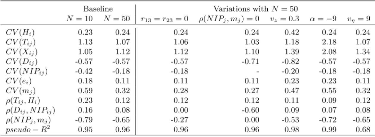
Method (5) is estimated on the whole dataset, constructed by the DGP described above, with N² observations including the intra-national dimension. Prior to estimation of the methods (1)-(4), the N observations corresponding to the intra-national trade flowsi=jare dropped. All methods are estimated by PPML, regardless of the underlying DGP variance function of a particular scenario. In each scenario, S = 10,000 replications of the DGP for a small (N = 10) and a medium-sized sample with N = 50 countries are performed. The impact of a particular scenario on some key properties of the generated data is summarized in Table (1).

The first scenario covers the baseline parametrization of the DGP given by α = −4, vz = 0.1, r12=r13=r23= 0.95, σ_η,ij² =vη×ln 1 +µ⁻¹_ij

andvη = 1. The left panel in Table (1) shows the data properties for the two sample sizes of the baseline scenario. The dispersion measured by the coefficient of variation (CV) increases with the sample size for the generated trade flowsXij, but decreases for the unobserved componentsei,mj and the non-discriminatory variableN IPj. Furthermore, a larger sample size reduces the correlation - denoted byρ(·,·) - between the total trade costsTij and endowmentsHias well as between N IP_j,D_ij andm_j, respectively.

In scenario 2, the correlation betweenN P I_j andm_jis reduced by setting the respective correlation of the latent variablesz_ij^H andz^D_ij withz_ij^{N IP}, i.e. r₁₃andr₂₃, to zero. The right panel of Table (1) summa- rizes the data properties for the sample sizeN = 50, when deviating form the baseline parametrization.

Setting r13 = r23 = 0 decreases the dispersion in mj and markedly reduces the correlation between N IPj andmj from -0.65 to -0.27. Since a major source of bias for methods without intra-national flows

will stem from this correlations, it is effectively set to zero in scenario 3. To achieve this, the DGP described above needs to be slightly modified. First, the auxiliary variables are drawn as before but disregardingz^{N IP}_ij in Eqs. (15) and (16). ThenN IPjis drawn form a standard normal distribution such that ρ(N IPj, mj) = 0.¹² Then construct lnTij =

exp(^zDij)

1+exp(^z_ij^D) ^−α/4

and deriveβDij = lnTij−γN IPij. Besides ensuringρ(N IPj, mj) = 0, this modification of the DGP further increases the dispersion ofDij, and introduces a substantial negative correlation between theDij andN IPij. The coefficient of variation is suppressed in Table (1) since N IPj has zero mean in this scenario.

The next two scenarios are taken from Egger & Staub (2016). Scenario 4 simulates the effects of an increased dispersion in endowments and trade flows, by setting v_z = 0.3. As shown in Table (1) this effectively increases the dispersion in all components of the structural part of the DGP. In scenario 5, a higher elasticity of substitution is assumed by setting α=−9. Compared to scenario 4, this exerts an even stronger impact on the dispersion of the trade costs and flows, which is nearly doubled.

Scenario 6 simulates additional noise in the stochastic component by increasing the variance in- flation factor of the error term vη. The baseline specification of vη = 1 leads to a pseudo-R² = V(µij)/[V(µij) +V(Xij−µij)] of around 0.95. Setting vη = 9 decreases this measure to an average of 0.68.

Table 1: Data Properties

Baseline Variations withN= 50

N= 10 N= 50 r13=r23= 0 ρ(N IPj, mj) = 0 vz= 0.3 α=−9 vη= 9

CV(Hi) 0.23 0.24 0.24 0.24 0.42 0.24 0.24

CV(Tij) 1.13 1.07 1.06 1.03 1.18 2.18 1.07

CV(Xij) 1.05 1.12 1.12 1.10 1.39 2.08 1.34

CV(Dij) -0.57 -0.57 -0.57 -0.71 -0.82 -0.57 -0.57

CV(N IPij) -0.42 -0.18 -0.18 - -0.20 -0.18 -0.18

CV(ei) 0.18 0.11 0.11 0.11 0.23 0.23 0.11

CV(mj) 0.59 0.32 0.28 0.27 0.47 0.55 0.32

ρ(Tij, Hi) 0.23 0.12 0.12 0.12 0.11 0.09 0.12

ρ(Dij, N IPij) 0.16 0.08 0.00 -0.60 0.09 0.07 0.08 ρ(N IPj, mj) -0.79 -0.65 -0.27 0.00 -0.53 -0.72 -0.65

pseudo−R² 0.95 0.96 0.96 0.96 0.98 0.99 0.68

Note: The table contains the mean statistics of 10,000 replications.

Following Head & Mayer (2014), the effects on the estimates if some proportion of the data is missing, as is often the case in empirical applications, are simulated in scenario 7. The DGP is simulated for a sample ofN = 100 countries and then 10 (50) countries are randomly selected. Estimation is performed on the sub-sample corresponding to observations containing the selected countries as exporter or importers.

Other than that, the baseline parametrization of the DGP is employed in this scenario.

In scenario 8, the robustness of the PPML estimator with respect to different assumptions of the variance process is assessed. In a GLM the choice of the linear exponential family distribution will lead

12First orthogonalize a standard normal variable (zj) to the centered and scaled effectmj, then scale both vectors to length one ( ˜mj, ˜zj) and compute ˜ζj= ˜zj+ 1/tan(arccos(r))∗m˜jfor an exact sample correlationr, withr= 0.

to a particular variance function, under which the estimator is asymptotically efficient. In the baseline scenario the errors are drawn from Eq. (22) with σ_η,ij² = ln 1 +µ⁻¹_ij

, resulting in V(xij) = µij, i.e.

a Poisson family. While the PPML is most frequently used in empirical research, other applied PML estimators include Gamma (see Santos Silva & Tenreyro, 2006; Mart´ınez-Zarzoso, 2013) and Negative Binomial (see Burger, Van Oort & Linders, 2009; Head, Mayer & Ries, 2009). Estimators of these families will be optimal in terms of efficiency ifσ_η,ij² = ln (2) andσ²_η,ij = ln 2 +µ⁻¹_ij

, respectively.¹³ As a robustness check for the PPML, it will be applied to a DGP with a Gamma or Negative Binomial¹⁴ variance function for the stochastic component. Changes in the error distribution will only affect the data properties via the dispersion in the generated trade flows and the pseudo-R². Specifying either a Gamma or a Negative Binomial family, increases the dispersion in trade flows to around 1.85 and decreases the pseudo-R²to 0.36 in both cases (not reported in Table (1)).

The MC results will be summarized by the mean bias of the estimate from the true value given by 1/SP

s(γ−γˆs) and the standard deviation of the estimate q

1/SP

s(ˆγs−1/SP

sγˆs)²for the coefficient estimates onD_ijandN IP_j, covering only replications in which the estimation algorithms of the respective method converged. The number of successful convergences in percent of total replications is given by CR.

3.3 Simulation Results

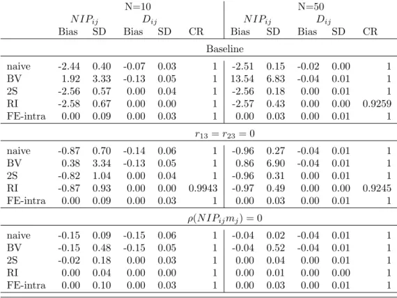
The upper panel in Table (2) summarizes the results for the baseline scenario. Recall that the methods naive, BV, 2S and RI are estimated on the sub-sample excluding intra-flows, while FE-intra is estimated on the full sample ofN²observations. The first column shows that all estimators disregarding the intra- national flows yield severely biased coefficient estimates on the non-discriminatory variableN IP_ij. Since the true value of the coefficient on the NDTP measure was set to one, the naive, 2S and RI method yield estimates that are biased downwards in a magnitude of more than 200%. Conversely, the BV estimate is biased upward by nearly 200% and results in by far the highest standard deviations. Increasing the sample size (right panel) has no noticeable effect on the bias of the naive, 2S and RI estimates, but decreases their respective standard deviation. The bias of the BV estimate is increased by a factor of 4 and the standard deviation is doubled. Note that for the medium-sized sample the random intercept model experiences converge failures of around 7.5% of the times.

By contrast, the FE-intra estimator results in virtually unbiased estimates of the coefficients on the NDTP variable. This result was to be expected, since this estimator adequately represents the underlying data generating process and exploits the identifying variation between the international and intra-trade flows. Besides being unbiased the FE-intra method yields the lowest standard deviation of the NDTP

13Note that Head & Mayer (2014) advised against the use of a Negative Binomial GLM, due to the scale dependency of its estimates, as shown in Bosquet & Boulhol (2014). Furthermore, Fally (2015) put forward that only the PPML with fixed effects automatically satisfies the constraints of the structural gravity model.

14As in Egger & Staub (2016), the over-dispersion parameter is fixed at 1.

variable, with the desirable asymptotic property of further decreasing with increasing sample size. Note that the effect on the discriminatory variable is estimated more efficiently than the estimate on NDTP, since the latter only is identified byN observations.

Turning to the results of the discriminatory variable Dij, the naive and BV method yield biased estimates as expected. The bias in the naive estimate is entirely due to the omission of the MRT. However, Egger & Staub (2016) note that as the sample size goes to infinity, the problem thatE(D_ije_i)6= 0 and E(D_ijm_j) 6= 0 will vanish and so will the bias of this misspecified model. While this is true for the discriminatory variable, the results in Table (2) indicate that the bias on the NDTP estimate will not vanish.¹⁵ As expected, the 2S and RI method yield unbiased and efficient estimates of the discriminatory trade cost variable, since they fully control for the MRT.

Table 2: MC results for baseline and reduced correlation scenarios

N=10 N=50

N IPij Dij N IPij Dij

Bias SD Bias SD CR Bias SD Bias SD CR

Baseline

naive -2.44 0.40 -0.07 0.03 1 -2.51 0.15 -0.02 0.00 1

BV 1.92 3.33 -0.13 0.05 1 13.54 6.83 -0.04 0.01 1

2S -2.56 0.57 0.00 0.04 1 -2.56 0.18 0.00 0.01 1

RI -2.58 0.67 0.00 0.00 1 -2.57 0.43 0.00 0.00 0.9259

FE-intra 0.00 0.09 0.00 0.03 1 0.00 0.03 0.00 0.01 1

r₁₃=r₂₃= 0

naive -0.87 0.70 -0.14 0.06 1 -0.96 0.27 -0.04 0.01 1

BV 0.38 3.34 -0.13 0.05 1 0.86 6.90 -0.04 0.01 1

2S -0.82 1.04 0.00 0.04 1 -0.96 0.31 0.00 0.01 1

RI -0.87 0.93 0.00 0.00 0.9943 -0.97 0.49 0.00 0.00 0.9245

FE-intra 0.00 0.09 0.00 0.03 1 0.00 0.03 0.00 0.01 1

ρ(N IPijmj) = 0

naive -0.15 0.09 -0.15 0.06 1 -0.04 0.02 -0.04 0.01 1

BV -0.15 0.48 -0.15 0.05 1 -0.04 0.52 -0.04 0.01 1

2S -0.02 0.18 0.00 0.03 1 0.00 0.04 0.00 0.01 1

RI 0.00 0.04 0.00 0.00 1 0.00 0.01 0.00 0.00 1

FE-intra 0.00 0.10 0.00 0.03 1 0.00 0.03 0.00 0.01 1

Note: All estimations are performed by PPML. Results are based on 10,000 replications.

The middle panel of Table (2) demonstrates the effect of decreasing correlation between the NDTP and the respective collinear effectm_j on the bias and efficiency of the methods. Compared to the upper panel, the bias of the effect on the NDTP variable is substantially reduced but still amounts to -87%

or +38%, depending on the method used. To push the argument even further, the lower panel in Table (2) shows the MC outputs when setting the sample correlation to zero. In this scenario, the RI method results in virtually unbiased estimates for the NDTP, even in small samples. The 2S estimate is only

15To illustrate the persistence of the bias on the NDTP estimate of the naive gravity model, see the MC results in Table (6) in the Appendix.

marginally biased in the small sample and unbiased up to the second digit in the medium-sized sample.

The naive gravity model and the BV estimates remains biased in a similar order of magnitude. In fact it can be demonstrated that assuming a constant variance σ²_η,ij = σ²_η in Eq. (22) of the DGP and applying OLS to a log-linearized version of Eq. (10) will result in unbiased estimates on N IPij and D_ij.¹⁶ Thus, the remaining bias on the BV estimates in this scenario is entirely due to the usage of a log-linear transformation in a multiplicative model set-up. This scenario clearly illustrated that the main source of bias in NDTP of the methods disregarding intra-national flows is due to the correlation between N IPj and the unobservedmj.

In the remaining scenarios, the correlation structure will correspond to the baseline scenario setting.

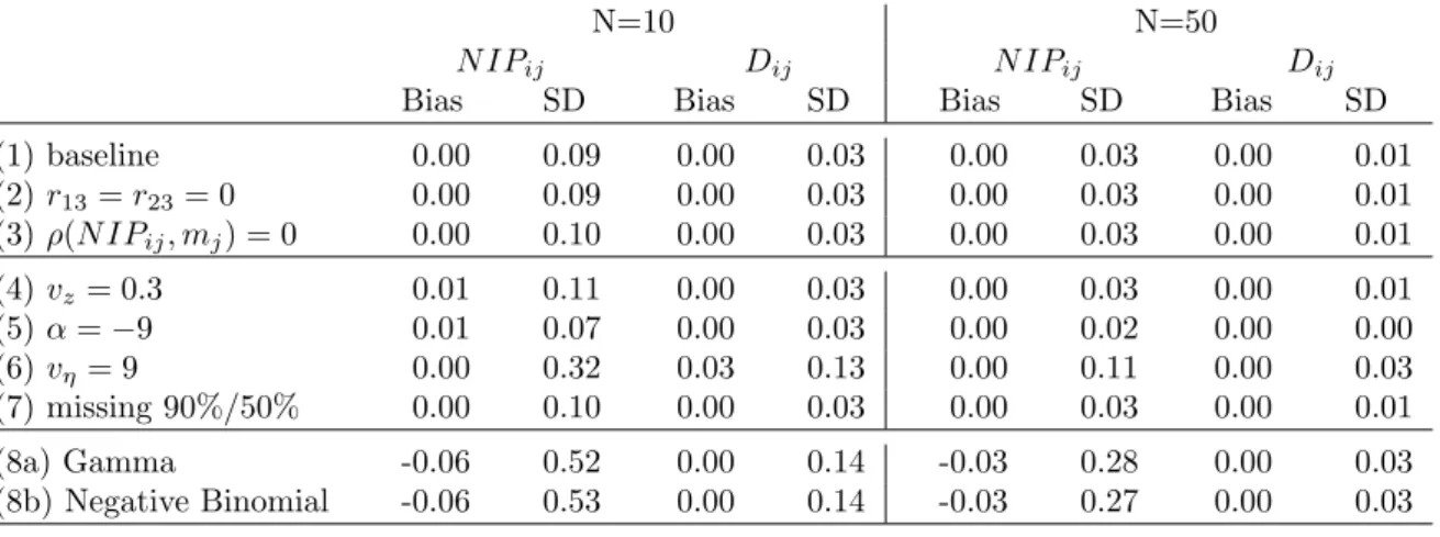
As the BV, 2S and RI method were severely biased in the baseline scenario, MC results for the remaining scenarios will only be reported for the FE-intra method, for brevity. Results for all methods are given in Table (7) in the Appendix. Table (3) shows the results of all eight scenarios for the FE-intra method only. The first three scenarios are repeated for comparison.

Increasing the overall dispersion of the latent variables or assuming a higher elasticity of substitution, see rows (4) and (5), introduces a marginal bias of 1% in the small sample. Settingv_z= 0.3 also slightly worsens the efficiency of NDTP estimate, while α= −9 mildly reduces the standard deviation of the NDTP estimate. Increasing the error variance, by setting v_η = 9, has a more pronounced effect on the efficiency of the estimate, as would be expected. Still, assuming a Poisson distribution in the DGP, the FE-intra method estimated by PPML leads to unbiased estimates of N IPij, even in the small sample.

Randomly dropping either 10% (left panel) or 50% (right panel) of the sample has virtually no effect on bias and efficiency (see row 7).

Table 3: MC results for FE-intra estimator for all scenarios

N=10 N=50

N IPij Dij N IPij Dij

Bias SD Bias SD Bias SD Bias SD

(1) baseline 0.00 0.09 0.00 0.03 0.00 0.03 0.00 0.01

(2)r₁₃=r₂₃= 0 0.00 0.09 0.00 0.03 0.00 0.03 0.00 0.01

(3)ρ(N IP_ij, m_j) = 0 0.00 0.10 0.00 0.03 0.00 0.03 0.00 0.01

(4)v_z= 0.3 0.01 0.11 0.00 0.03 0.00 0.03 0.00 0.01

(5)α=−9 0.01 0.07 0.00 0.03 0.00 0.02 0.00 0.00

(6)vη= 9 0.00 0.32 0.03 0.13 0.00 0.11 0.00 0.03

(7) missing 90%/50% 0.00 0.10 0.00 0.03 0.00 0.03 0.00 0.01

(8a) Gamma -0.06 0.52 0.00 0.14 -0.03 0.28 0.00 0.03

(8b) Negative Binomial -0.06 0.53 0.00 0.14 -0.03 0.27 0.00 0.03 Note: All estimations are performed by PPML. Results are based on 10,000 replications.

In scenario eight, the DGP assumes a variance function that corresponds to a Gamma-PML (8a) or Negative Binomial PML (8b) as an efficient estimator. Since the conditional mean function is correctly

16See Table (5) in the Appendix.

specified in the PPML, the estimates should be unbiased and consistent. For both variance assumptions, estimates on the NDTP show a small sample bias of 6%, that reduces to 3% in the medium-sized sample.

By contrast, the discriminatory variable is estimated without bias even in the small sample. In the small sample, the standard deviations of both estimates are increased by a factor of 5 compared to the baseline scenario. Increasing the sample size toN = 50 decreases the standard deviation on the NDTP measure by around 40%. Still, compared to the estimate on the discriminatory measure, the effect of NDTP is estimated less efficiently, as expected from a GLM with misspecified variance function.

4 Empirical Application

This section illustrates the methods discussed above in an empirical application. It should be noted that it is not the purpose of this application to derive exact estimates on the effects of the trade cost variables used, but to demonstrate the impact of the methods on the estimates of the NDTP variable.

For a thorough analysis of the effects of trade policy measures on trade flows in structural gravity model, the challenges summarized in Piermartini & Yotov (2016) should be adequately addressed. On the issue of intra-national trade flow data, Piermartini & Yotov (2016) note that because such data will not be readily available, their use requires caution. The following application will therefore be based on an existing database, namely CEPII’s ’TradeProd’ (see de Sousa, Mayer & Zignago, 2012), that covers approximately 150 countries between 1980-2006 at a 3-digit level of the ISIC Revision 2 manufacturing industries.

TradeProd includes data on production, consumption as well as internal and international trade flows. Since trade flows and internal consumption are not available for the ISIC aggregation 300 ’total manufacturing’, an industry and a year is chosen that maximized the sample size with respect to data availability. This led to the selection of the industry 311 ’Food products’ and the year 2000, resulting in a total of 63 countries. Including data on intra-national flows a total of 3,963 observations is available, leading to sample of 3,900 observations for the estimators disregarding the intra-national flows (naive, BV, 2S and RI).

As a measure of non-discriminatory trade policy the most-favoured nation (MFN) tariff was selected.

The MFN for the year 2000, calculated as a weighted mean of food products, was taken from the UNCTAD TRAINS database accessed via the World Integrated Trade Solution (WITS) website. As is common practice with data on tariffs, the variable will be included as ln(M F N_ij + 1). Data on geographical distances¹⁷, shared borders and common language¹⁸ is taken from the CEPII GeoDist database (see Mayer & Zignago, 2011) and information on regional trade agreements is obtained from ’Mario Larchs Regional Trade Agreements Database’ (see Egger & Larch, 2008). Shared borders (BORDERij), common

17Bilateral and internal distances are measured by the distances between the main agglomerations, between and within countries, weighted by their population share.

18This dummy variable takes the value one if countries share either an ethnic or official language and zero otherwise.

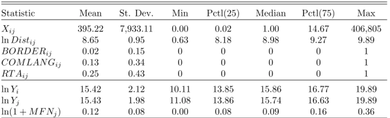
language (COM LAN Gij) and regional trade agreements (RT Aij) enter as dummy variables and distances are included in logarithms (lnDistij). The descriptive statistics of the data are summarized in Table (8) in the Appendix.

In the application, the production and consumption coefficients are not restricted to unity, so the Bonus-Vetus method (BV) and the non-structural model (naive) include these additional variables in logarithms. In the second stage of the two-stage fixed effect method (2S), the antilogs of the fixed effects of the importer countries are regressed onto the MFN measure and the log of consumption. All methods are estimated via PPML and standard errors reported are heteroscadsticity-robust sandwich estimates, except for the random intercept PPML method (RI). The fixed effects model on the sample including the intra-national trade flows (FE-intra) was estimated including a ’home’/’same country’ dummy variable that takes value one for intra-national flows and zero otherwise (as in Heid et al., 2015).

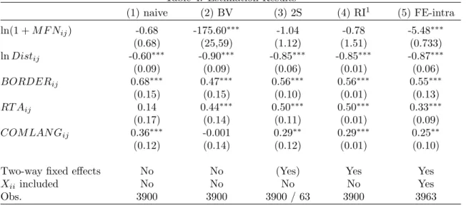
Table 4: Estimation Results

(1) naive (2) BV (3) 2S (4) RI¹ (5) FE-intra

ln(1 +M F Nij) -0.68 -175.60^∗∗∗ -1.04 -0.78 -5.48^∗∗∗

(0.68) (25,59) (1.12) (1.51) (0.733)

lnDistij -0.60^∗∗∗ -0.90^∗∗∗ -0.85^∗∗∗ -0.85^∗∗∗ -0.87^∗∗∗

(0.09) (0.09) (0.06) (0.01) (0.06)

BORDER_ij 0.68^∗∗∗ 0.47^∗∗∗ 0.56^∗∗∗ 0.56^∗∗∗ 0.55^∗∗∗

(0.15) (0.15) (0.10) (0.01) (0.13)

RT A_ij 0.14 0.44^∗∗∗ 0.50^∗∗∗ 0.50^∗∗∗ 0.33^∗∗∗

(0.17) (0.14) (0.11) (0.01) (0.09)

COM LAN Gij 0.36^∗∗∗ -0.001 0.29^∗∗ 0.29^∗∗∗ 0.25^∗∗

(0.12) (0.14) (0.12) (0.01) (0.10)

Two-way fixed effects No No (Yes) Yes Yes

Xii included No No No No Yes

Obs. 3900 3900 3900 / 63 3900 3963

Note: All estimations were performed by PPML with heteroscedasticity-robust sandwich standard errors (except for random intercept model). ¹Robust standard errors are currently not supported for generalised linear mixed models in the lme4 package. ^∗p<0.1;^∗∗p<0.05;

∗∗∗p<0.01

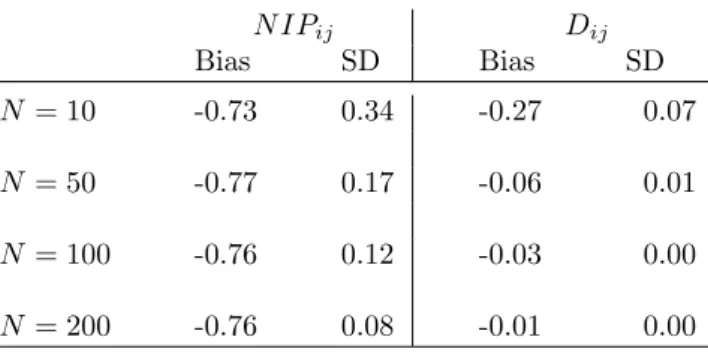
The estimates on the coefficients corresponding to all methods are reported in Table (4). Size and sign of the coefficients on distance, border, regional trade agreement and common language are comparable to the meta-study values given in Head & Mayer (2014). As a benchmark for comparison on the size, sign and standard error of the coefficient on the MFN, the FE-intra method in column (5), as the best performing method from the MC simulations, is chosen. As expected, the MFN has a negative impact on bilateral trade flows, which is estimated at -5.48, a value very similar to the one estimated for food products in Heid et al. (2015). The coefficient is precisely estimated, with a heteroscedasticity-robust standard error of 0.73, and is highly significant at conventional levels.

The other four methods, disregarding intra-national trade flows, all yield negative coefficients with varying sizes and precision. As shown in the MC simulations, given a positive true coefficient, the