• Keine Ergebnisse gefunden

Quantitative Estimation of Surface Soil Moisture in Agricultural Landscapes using Spaceborne Synthetic Aperture Radar Imaging at Different Frequencies and Polarizations

N/A
N/A
Protected

Academic year: 2021

Aktie "Quantitative Estimation of Surface Soil Moisture in Agricultural Landscapes using Spaceborne Synthetic Aperture Radar Imaging at Different Frequencies and Polarizations"

Copied!
229
0
0

Wird geladen.... (Jetzt Volltext ansehen)

Volltext

(1)

Quantitative Estimation of Surface Soil Moisture in Agricultural Landscapes using

Spaceborne Synthetic Aperture Radar Imaging at Different Frequencies and

Polarizations

Inaugural-Dissertation zur

Erlangung des Doktorgrades

der Mathematisch-Naturwissenschaftlichen Fakultät der Universität zu Köln

vorgelegt von

Christian Naohide Koyama aus Bergisch-Gladbach

2012

(2)

Berichterstatter: Prof. Dr. Karl Schneider

Prof. Dr. Georg Bareth

Tag der mündlichen Prüfung: 27.01.2012

(3)

Abstract

Abstract

Soil moisture and its distribution in space and time plays an important role in the surface energy balance at the soil-atmosphere interface. It is a key variable influencing the partitioning of solar energy into latent and sensible heat flux as well as the partitioning of precipitation into runoff and percolation. Due to their large spatial variability, estimation of spatial patterns of soil moisture from field measurements is difficult and not feasible for large scale analyses. In the past decades, Synthetic Aperture Radar (SAR) remote sensing has proven its potential to quantitatively estimate near surface soil moisture at high spatial resolutions. Since the knowledge of the basic SAR concepts is important to understand the impact of different natural terrain features on the quantitative estimation of soil moisture and other surface parameters, the fundamental principles of synthetic aperture radar imaging are discussed. Also the two spaceborne SAR missions whose data was used in this study, the ENVISAT of the European Space Agency (ESA) and the ALOS of the Japanese Aerospace Exploration Agency (JAXA), are introduced. Subsequently, the two essential surface properties in the field of radar remote sensing, surface soil moisture and surface roughness are defined, and the established methods of their measurement are described. The in situ data used in this study, as well as the research area, the River Rur catchment, with the individual test sites where the data was collected between 2007 and 2010, are specified. On this basis, the important scattering theories in radar polarimetry are discussed and their application is demonstrated using novel polarimetric ALOS/PALSAR data. A critical review of different classical approaches to invert soil moisture from SAR imaging is provided. Five prevalent models have been chosen with the aim to provide an overview of the evolution of ideas and techniques in the field of soil moisture estimation from active microwave data. As the core of this work, a new semi-empirical model for the inversion of surface soil moisture from dual polarimetric L-band SAR data is introduced. This novel approach utilizes advanced polarimetric decomposition techniques to correct for the disturbing effects from surface roughness and vegetation on the soil moisture retrieval without the use of a priori knowledge.

The land use specific algorithms for bare soil, grassland, sugar beet, and winter wheat allow

quantitative estimations with accuracies in the order of 4 Vol.-%. Application of remotely

sensed soil moisture patterns is demonstrated on the basis of mesoscale SAR data by

(4)

Abstract

investigating the variability of soil moisture patterns at different spatial scales ranging from

field scale to catchment scale. The results show that the variability of surface soil moisture

decreases with increasing wetness states at all scales. Finally, the conclusions from this

dissertational research are summarized and future perspectives on how to extend the proposed

model by means of improved ground based measurements and upcoming advances in sensor

technology are discussed. The results obtained in this thesis lead to the conclusion that state-

of-the-art spaceborne dual polarimetric L-band SAR systems are not only suitable to

accurately retrieve surface soil moisture contents of bare as well as of vegetated agricultural

fields and grassland, but for the first time also allow investigating within-field spatial

heterogeneities from space.

(5)

Kurzzusammenfassung

Kurzzusammenfassung

Bodenfeuchte und deren Verteilung in Raum und Zeit spielt eine wichtige Rolle in der

Energiebilanz an der Erdoberfläche. Sie beeinflusst die Partitionierung von Sonnenenergie in

latenten und fühlbaren Wärmefluss sowie die Aufteilung des Niederschlags in Abfluss und

Versickerung. Aufgrund ihrer hohen räumlichen Variabilität, ist die Bestimmung von

räumlichen Bodenfeuchtemustern anhand von Feldmessungen schwierig und für großräumige

Untersuchungen nicht praktikabel. In den vergangenen Jahrzehnten hat die Fernerkundung

mittels Radar mit Synthetischer Apertur (SAR) ihr Potenzial zur quantitativen Bestimmung

der oberflächennahen Bodenfeuchte mit hoher räumlicher Auflösung erwiesen. Da

Kenntnisse über die grundlegenden Eigenschaften der SAR-Fernerkundung wichtig sind, um

die Auswirkungen der verschiedenen natürlichen Oberflächen- und Geländeeigenschaften auf

die Berechnung der Bodenfeuchte und anderer Oberflächen-Parameter zu verstehen, werden

die grundlegenden Prinzipien der SAR Bildgebung diskutiert. In diesem Zusammenhang

werden auch die beiden SAR-Satelliten, deren Daten in dieser Studie Verwendung finden, der

ENVISAT der europäischen Weltraumorganisation (ESA) und der ALOS der japanischen

Weltraumorganisation (JAXA), vorgestellt. Anschließend werden die beiden zentralen

Oberflächeneigenschaften im Bereich der Radar-Fernerkundung, die Bodenfeuchte und die

Bodenrauhigkeit, detailliert erklärt, und die etablierten Messmethoden beschrieben. Die in

dieser Studie verwendeten in situ Daten, sowie das Untersuchungsgebiet, das Rur

Einzugsgebiet mit den einzelnen Test-Standorten, an denen die Daten in den Jahren 2007 -

2010 erhoben wurden, werden beschrieben. Auf dieser Grundlage werden die wichtigen

Rückstreuungstheorien in der Radar Polarimetrie diskutiert und ihre Anwendung anhand

neuartiger polarimetrischen ALOS/PALSAR Daten gezeigt. Eine kritische Betrachtung

verschiedener klassischer Ansätze zur Berechnung der Bodenfeuchte aus SAR Daten erfolgt

am Beispiel unterschiedlicher Modelle, welche mit dem Ziel ausgewählt wurden, einen

Überblick über die Entwicklung von Ideen und Techniken auf dem Gebiet der

Bodenfeuchtebestimmung mit aktiven Mikrowellen-Sensoren zu geben. Als Kernstück dieser

Arbeit wird ein neues semi-empirisches Modell für die Inversion der

Oberflächenbodenfeuchte mit dual polarimetrischen L-Band SAR Daten vorgestellt. Dieser

neuartige Ansatz nutzt polarimetrische Dekompositionstechniken um die störenden Einflüsse

(6)

Kurzzusammenfassung

von Bodenrauhigkeit und Vegetation auf die Bodenfeuchteibestimmung ohne Zuhilfenahme von a-priori Informationen zu korrigieren. Die landnutzungsspezifischen Algorithmen für Grasland, unbedeckten Boden, Winterweizen und Zuckerrüben ermöglichen eine Abschätzungsgenauigkeit im Bereich von ±4 Vol.-%. Als Anwendungsbeispiel für fernerkundlich bestimmte Bodenfeuchtemuster, wird auf der Grundlage mesoskaliger SAR Daten die Variabilität der Oberflächenbodenfeuchte auf unterschiedlichen räumlichen Skalen untersucht. Es wird gezeigt, dass die Variabilität der räumlichen Bodenfeuchteverteilung auf allen Skalen mit zunehmendem Feuchtezustand der Bodenoberfläche kleiner wird.

Schließlich werden die Schlussfolgerungen aus dieser Doktorarbeit zusammengefasst und es

werden Zukunftsperspektiven, wie das vorgestellte Modell durch verbesserte bodengestützte

Messungen und kommende Entwicklungen in der Sensor-Technologie erweitert werden kann,

diskutiert. Die Ergebnisse dieser Arbeit zeigen, dass moderne, weltraumgestützte dual

polarimetrische L-band SAR Systeme nicht nur eine genaue Bestimmung der Bodenfeuchte

auf nackten und vegetationsbedeckten landwirtschaftlich genutzten Flächen ermöglichen,

sondern zum ersten Mal auch eine kleinräumige Untersuchung von Heterogenitäten innerhalb

einzelner Ackerschläge erlauben.

(7)

Acknowledgements

Acknowledgements

The present thesis was prepared during the first phase of the Transregional Collaborative Research Center 32 (SFB/TR32) “Patterns in Soil-Vegetation-Atmosphere Systems:

Monitoring, Modeling, and Data Assimilation", funded by the German Research Foundation (DFG). This financial support is gratefully acknowledged. Besides, the European Space Agency (ESA) and the Japanese Aerospace Exploration Agency (JAXA) are greatly thanked for the provision of ENVISAT ASAR and ALOS PALSAR data through their PI program (AOALO.3570).

The thesis was supervised by Prof. Dr. Karl Schneider, to whom I owe my sincere gratitude not only for giving me the chance to participate in the research project and for introducing me to the truly fascinating and challenging field of radar remote sensing, but also for his guidance and invaluable suggestions for improving my work.

I thank Prof. Dr. Bareth for his consent to act as second examiner, as well as for his motivating words whenever we talked. Special gratitude is also expressed to Prof. Dr.

Susanne Crewell for chairing the examination committee and more.

I am grateful to all colleagues within the project for their friendly and fruitful collaboration.

A very special thank you is due to Dr. Stefan Kollet who not only strongly supported me in his role as scientific coordinator, but who also became a good friend. Moreover, I would also like to thank Prof. Dr. Clemens Simmer and Dr. Karin Boessenkool, for their support.

I thank Dr. Carsten Montzka and Guido Waldhoff for the provision of the land use

classifications. Dirk Hoffmeister is greatly thanked for the help with the 3D surface

roughness measurements. Gratitude is also owed to Dr. Lutz Damerow from the Technology

of Crop Farming Institute of the University of Bonn for making the prototype laser scanner

available to this study.

(8)

Acknowledgements

My very special gratitude goes to Dr. Masanobu Shimada, ALOS Science Project Manager at JAXA/EORC, for the quick and cordial responses to my questions concerning the “Daichi”

and for providing me with lots of insider information during the friendly conversations at various conferences.

I thank the numerous student assistants who spent so much time with me in the field during the measurement campaigns and without whose help this work could not have been accomplished. Many thanks also go to all the farmers who made their fields available to us.

Finally yet importantly, my most heartfelt thanks go to my parents, Brigitta and Shoji, for

everything.

(9)

Contents

Contents

Abstract ... III Kurzzusammenfassung ... V Acknowledgements ... VII Contents ... IX List of Figures ... XII List of Tables ... XVI List of Abbreviations ... XVII

1. Introduction ... 1

1.1 Spaceborne Active Microwave Remote Sensing of Soil Moisture ... 3

1.2 Scope and Outline of the Thesis ... 5

2. Remote Sensing with Synthetic Aperture Radar Imaging ... 8

2.1 Development of Imaging Radar ... 9

2.2 Principles of Synthetic Aperture Radar ... 10

2.2.1 Radar Penetration Depth ... 12

2.3 SAR Imaging Geometry ... 13

2.4 SAR Spatial Resolution ... 15

2.5 SAR Complex Images ... 18

2.6 Radar Backscattering Coefficient ... 22

2.7 Speckle ... 24

2.8 ENVISAT-1 ASAR ... 26

2.8.1 Basic Processing of ASAR Data ... 29

2.9 ALOS PALSAR ... 31

3. Soil Surface Physical Properties ... 36

3.1 Soil Moisture Content ... 36

3.1.1 Unique Properties of Water ... 39

3.1.2 Complex Dielectric Constant ... 41

3.1.3 Measurement of Soil Moisture ... 44

3.1.4 Gravimetric Soil Moisture Determination ... 44

3.1.5 Frequency Domain Reflectometry ... 46

(10)

Contents

3.2 Surface Roughness ... 49

3.2.1 Statistical Description of Rough Surfaces ... 52

3.2.2 Methods of Surface Roughness Measurement ... 56

3.2.3 Electromagnetic Scattering from Rough Surfaces ... 58

4. Study Area and Field Measurements ... 63

4.1 The River Rur Catchment ... 63

4.1.1 Precipitation Characteristics of the Rur Catchment ... 64

4.1.2 Geological Overview ... 66

4.2 Test Sites and Sampling Fields ... 66

4.2.1 Test Site Selhausen ... 67

4.2.2 Test Site Rollesbroich ... 68

4.2.3 Test Site Duerwiss ... 70

4.3 Ground Truth Data Set ... 71

4.3.1 In Situ Surface Soil Moisture ... 71

4.3.2 In Situ Surface Roughness ... 74

4.3.3 In Situ Vegetation Parameters ... 77

5. Polarimetric Radar Imaging and the H / A /α Decomposition Theorem ... 79

5.1 Diagonalization of the Coherency [T 3 ] Matrix ... 80

5.2 Polarimetric Scattering Alpha Angle ... 81

5.3 Polarimetric Scattering Entropy ... 83

5.4 Polarimetric Scattering Anisotropy ... 84

5.5 Scattering Mechanism Interpretation... 85

5.6 ALOS PALSAR Experimental PolSAR Data Analysis ... 91

5.7 ALOS PALSAR Dual Polarimetric Decomposition ... 96

5.9.1 The Dual Polarized Entropy/Alpha Decomposition ... 97

5.9.3 Experimental Observations ... 99

6. Classical Models for Quantitative Soil Moisture Estimation ... 102

6.1 Theoretical Scattering Models ... 103

6.1.1 The Small Perturbation Model ... 104

6.1.2 The Integral Equation Model ... 106

6.2 Semi-empirical Inversion Models ... 109

6.2.1 The Oh Model ... 110

6.2.2 The Dubois Model ... 113

(11)

Contents

6.3 Empirical Retrieval Models ... 115

6.3.1 Empirical Soil Moisture Retrieval Model for Single Channel ASAR Data ... 116

6.3.2 Radar-Vegetation Interactions ... 118

6.4 The Need for a New L-band Model ... 122

7. A New Semi-Empirical Soil Moisture Model for Dual Polarimetric L-band SAR Data ... 124

7.1 Dual Polarimetric ALOS PALSAR Data ... 125

7.2 Preprocessing of Polarimetric PALSAR Data ... 126

7.2 Bare Soil Model ... 130

7.2.1 Surface Roughness Estimation ... 131

7.2.2 Soil Moisture Estimation on Bare Soil using Roughness Corrections ... 133

7.3 Grassland Model ... 134

7.3.1 Soil Moisture Estimation under Grassland Vegetation ... 136

7.4 Sugar Beet Model ... 138

7.4.1 Sugar Beet Biomass Estimation... 139

7.4.2 Soil Moisture Estimation using Sugar Beet Biomass Corrections ... 141

7.5 Winter Wheat Model ... 143

7.5.1 Winter Wheat Biomass Estimation ... 143

7.5.2 Soil Moisture Estimation using Winter Wheat Biomass Corrections ... 145

7.6 PALSAR Soil Moisture Maps ... 147

8. Variability of Surface Soil Moisture ... 151

8.1 Soil Moisture Patterns ... 151

8.2 Statistical Description of Soil Moisture Variability ... 153

8.3 ASAR Derived Soil Moisture Patterns ... 154

8.4 Analysis of Soil Moisture Variability ... 155

9. Conclusions and Perspectives ... 162

References ... 168

Appendix ... 191

(12)

List of Figures

List of Figures

Figure 2.1: Microwave section of the electromagnetic spectrum. ... 9

Figure 2.2: Schematic representation of radar penetration into vegetation and soil at L- and C-band (redrawn after Ulaby et al., 1981b). ... 13

Figure 2.3: SAR imaging geometry in strip-map mode. ... 14

Figure 2.4: Broadside view of the SAR geometry in altitude ground-range domain. ... 15

Figure 2.5: Broadside view of the SAR geometry in slant-range azimuth domain. ... 15

Figure 2.6: Geometric effects of terrain slope variations. ... 18

Figure 2.7: Schematic representation of the ground range to slant range projection. ... 20

Figure 2.8: Foreshortening effect. ... 21

Figure 2.9: Layover effect. ... 21

Figure 2.10: Radar shadow effect. ... 22

Figure 2.11: Schematic illustration of distributed targets and imaging geometry. ... 25

Figure 2.12: Coherent sum of discrete scatterers within one image pixel. ... 26

Figure 2.13: ENVISAT-1 in orbit (left) and the ASAR aperture in the laboratory (right); ... 27

Figure 2.14: Basis processing chain for ENVISAT-1 ASAR data. ... 29

Figure 2.15: ALOS PALSAR in orbit (left) and in the laboratory (right); ... 32

Figure 2.16: The Selhausen test site in ASAR Image Mode VV polarization (left) and PALSAR Fine Beam Mode HV polarization (right). ... 34

Figure 3.1: Generic relationship between water content and suction for a sand, a silt, and a clay texture (redrawn after Scheffer & Schachtschabel, 2002) ... 39

Figure 3.2: Top view of the vadose zone with predominant forces restraining water in the soil. ... 40

Figure 3.3: Schematic representation of the stick cylinder technique. ... 45

Figure 3.4: Frequency domain reflectometry scheme. ... 47

Figure 3.5: Concept of electromagnetic wave scattering on rough surfaces (Cloude, 1999). ... 54

Figure 3.6: Devices for the measurement of the soil surface roughness: a) classical pin meter, b) field laser scanner, and c) terrestrial 3D laser scanner. ... 58

Figure 3.7: Schematic representation of Fresnel reflection. ... 59

Figure 3.8: Characterization of roughness components on a) smooth, b) rough, and c) very rough

surfaces. ... 60

(13)

List of Figures

Figure 3.9: Scheme for the determination of the phase difference between two parallel EM waves

scattered from different points on a rough surface. ... 61

Figure 4.1: River Rur catchment with the two major landscape units (grey shaded) and locations of the three test sites for in situ soil moisture measurements. ... 64

Figure 4.2: Distribution of annual precipitation in the Rur catchment; ... 65

Figure 4.3: Aerial view of the Selhausen test site. ... 68

Figure 4.4: Aerial view of the Rollesbroich test site. ... 69

Figure 4.5: Aerial view of the Duerwiss test site... 70

Figure 4.6: Continuous surface soil moisture measurements with TDR (Rollesbroich, G03) and FDR (Selhausen, A10) probes in 10 cm depth. ... 74

Figure 4.7: Terrestrial laser scanner 3D composite image of field A01 on May 4, 2008. ... 76

Figure 4.8: Tower view of the test field A11 with seedbed (left) and ploughed surface (right). ... 77

Figure 5.1: Schematic representation of the α angle interpretation. ... 88

Figure 5.2: ALOS PALSAR Pauli-RGB of the River Rur catchment. The Pauli vectors are color coded as red = |HH-VV|, green = |HV-VH|, and blue = |HH+VV|. ... 93

Figure 5.3: Polarimetric entropy (left), anisotropy (middle), and alpha angle maps (right) of the River Rur catchment. ... 94

Figure 5.4: The Poincaré sphere interpretation of the dual polarized alpha angle. ... 97

Figure 5.5: Land use specific PALSAR dual-pol H2α planes for different imaging dates; mv is the mean surface soil moisture in Vol.-%, ks is the surface roughness, and SD is the corresponding standard deviation. ... 100

Figure 5.6: HSV image of the Selhausen test site from 21st July 2009 ... 101

Figure 6.1: Pixel-wise comparison between estimated and measured m v using the IEM. ... 109

Figure 6.2: Soil moisture distribution on field D01 in the Duerwiss test site on May 14. ... 109

Figure 6.3: Pixel-wise comparison between estimated and measured mv using the Oh model. ... 112

Figure 6.4: Surface soil moisture distribution on field D01 in the Duerwiss test site. ... 112

Figure 6.5: Pixel-wise comparison between estimated and measured mv using the Dubois model. 115 Figure 6.6: Soil moisture distribution on field D01 in the Duerwiss test site on May 14, 2009 ... 115

Figure 6.8: Comparison between measured and a) ASAR WS derived and b) ASAR IM derived surface soil moisture. ... 120

Figure 6.7: Soil moisture distribution map of the Rur catchment on 25 March 2008 as derived from ASAR WS image. ... 120

Figure 7.1: Simplified processing chain for dual polarized ALSO PALSAR data. ... 127

(14)

List of Figures

Figure 7.2: Dual polarization image set of the Selhausen area as obtained from PALSAR FBD data with

a) HH, b) HV, c) span, d) entropy, e) anisotropy, and f) alpha angle. ... 130

Figure 7.3: Comparison between HV/HH ratio and measured ks. ... 131

Figure 7.4: Comparison between anisotropy A and measured ks. ... 132

Figure 7.5: Comparison between estimated and measured ks. The bars indicate the corresponding standard deviations... 133

Figure 7.6: Comparison between measured and estimated m v before (left) and after surface roughness correction (right). ... 134

Figure 7.7: Schematic representation of the different scattering contributions occurring in a grassland pixel. ... 136

Figure 7.8: Grassland parameter model vs. measured dielectric constant. ... 137

Figure 7.9: Comparison between measured and estimated m v for grassland pixels on various dates. ... 138

Figure 7.10: Schematic representation of the different scattering contributions occurring in a sugar beet pixel. ... 139

Figure 7.11: Comparison between effective biomass parameter M BETA and measured total fresh weight of sugar beet biomass. ... 140

Figure 7.12: Estimated vs. measured total fresh weight of sugar beet biomass. ... 141

Figure 7.13: Estimated versus measured soil moisture for sugar beet pixels on various dates. ... 142

Figure 7.14: Winter wheat biomass parameter model vs. above ground fresh weight. ... 144

Figure 7.15: Estimated vs. measured above ground fresh weight winter wheat biomass. ... 145

Figure 7.16: Comparison between estimated and measured m v for winter wheat pixels. ... 146

Figure 7.17: PALSAR derived surface soil moisture patterns for the Selhausen sampling fields on June 22 (left) and September 5, 2009 (right). ... 148

Figure 7.18: PALSAR derived surface soil moisture patterns for the grassland test site Rollesbroich on July 18, 2008 (left) and July 21, 2009 (right). ... 149

Figure 7.19: PALSAR derived surface soil moisture distribution in the Rur catchment on June 22, 2009. ... 150

Figure 8.1: Envisat ASAR derived soil moisture pattern of the River Rur catchment from March 25, 2008. ... 155

Figure 8.2: Relationship between ASAR derived mean soil moisture and the CV for the entire River Rur catchment. ... 156

Figure 8.3: Relationship between ASAR derived soil moisture and coefficient of variation for the

fertile loess plain (left), and the low mountain range region (right). ... 157

(15)

List of Figures

Figure 8.4: Relationship between ASAR derived soil moisture and coefficient of variation for (a) the fertile loess plain pixels taking into account all dates and land cover classes. ... 158 Figure 8.5: Relationship between field mean soil moisture and coefficient of variation from in situ

measurements at the Selhausen test site. ... 159 Figure 8.6: Overview of the scale dependent relationships between coefficient of variation and

surface mean soil moisture. ... 160 Figure 9.1: Within-field variability of surface soil moisture distribution as seen by ALOS PALSAR. ... 165 Figure A.0.1: Propagation of a plane EM wave in direction k ... 194 Figure A.0.2: Different shapes of the polarization ellipse expressing the polarization states of a plane

wave. ... 195

Figure A.0.3: Full Poincaré sphere with wave amplitude A, absolute phase α, ... 196

Figure A.0.4: Back-Scattering Alignment (BSA) geometry. ... 201

(16)

List of Tables

List of Tables

Table 2.1: ASAR instrument parameters... 28

Table 2.2: PALSAR instrument parameters ... 32

Table 4.1: Corner coordinates of the Selhausen test site. ... 67

Table 4.2: Corner coordinates of the test site Rollesbroich. ... 68

Table 4.3: Corner coordinates of the test site Duerwiss... 70

Table 4.4: Overview of measured average surface soil moisture for the different land cover types and dates of ASAR and PALSAR acquisitions. ... 72

Table 4.5: Measured surface roughness for different test fields and dates. ... 75

Table 5.1: Angular values of canonical targets ( ∞ represents non-fixed values). ... 89

Table 5.2: Land cover type specific ranges of values for polarimetric target parameters. ... 95

Table 6.1: Land use dependant coefficients for the inversion of σ 0 to ε′ using (6.20) and biomass correction coefficients for (6.21) at an incidence angle of 23°. (Loew et al., 2006) ... 117

Table 7.1: PALSAR data and associated field measurements (m v , s, and v represent measurements of soil moisture, RMS height, and vegetation parameters, respectively). ... 125

Table A.0.1: Characteristic polarization states with corresponding polarization descriptors. ... 195

(17)

List of Abbreviations

List of Abbreviations

ALOS Advanced Land Observing Satellite

AOI Angle Of Incidence

ASAR Advanced Synthetic Aperture Radar

CAS Canadian Space Agency

CAL/VAL Calibration/Validation

CCRS Canadian Centre of Remote Sensing CEOS Committee on Earth Observing Satellites

dB decibel

DC Dielectric Constant

DEM Digital Elevation Model

DInSAR Differential Interferometric Synthetic Aperture Radar DLR Deutsches Zentrum für Luft- und Raumfahrt

DN Digital Number

EM electromagnetic

EO Earth Observation

EORC Earth Observation Research Center

ERS European Remote sensing Satellite

ESA European Space Agency

FBD Fine mode Beam Dual-polarimetric

FBS Fine mode Beam Single-polarimetric

FDR Frequency Domain Reflectometry

GIS Geographical Information System

GNSS Global Navigation Satellite System

GOM Geometric Optics Model

GPS Global Positioning System

HSV Hue/Saturation/Value

IEM Integral Equation Model

IPU International Physical Union

JAXA Japanese Aerospace Exploration Agency

JERS Japanese Earth Resources Satellite

(18)

List of Abbreviations

JPL Jet Propulsion Laboratory

KA Kirchhoff Approximation

LAI Leaf Area Index

LANDSAT Land Satellite

LIA Local Incidence Angle

LiDAR Light Detecting And Ranging

LOS Line Of Sight

NASA National Aeronautics and Space Administration NDVI Normalized Difference Vegetation Index

PALSAR Phased Array type L-band Synthetic Aperture Radar PAR parallel to the row direction

POM Physic Optics Model

PolSAR Polarimetric Synthetic Aperture Radar

PolInSAR Polarimetric Interferometry Synthetic Aperture Radar PPR perpendicular to the row direction

RADAR Radio Detecting And Ranging

RADARSAT Radar Satellite

RCS Radar Cross Section

RGB Red/Blue/Green

RLA Radar Look Angle

RLOS Radar Line Of Sight

RMS Root Mean Square

SAR Synthetic Aperture Radar

SNR Signal-to-Noise Ratio

SLC Single Look Complex

SPM Small Perturbation Model

SPOT Satellite Probatoire d’Observation de la Terre

TDR Time Domain Reflectometry

T/R Transmit/Receive

UAV Unmanned Airborne Vehicle

UTM Universal Transverse Mercator

WS Wide Swath

(19)

Introduction

1. Introduction

Without any doubt, soil moisture can be regarded as one of the important life sustaining entities on our planet. Among its various functions, the first is probably to enable the growth of vegetation on the land surface. Apart from this, water stored in soils has several others roles in the global water cycle. For instance, it controls the partitioning of rainfall into runoff and infiltration, where efficient infiltration commonly means replenishment of aquifers, while runoff may mean both exportation of valuable fresh water to other areas and degradation of top soil through leaching and erosion. The saturation state of a soil may also affect the transformation of rainfall into floods. Thus, surface soil moisture is a key variable for improving the forecasting performance of run-off models in terms of flood risk assessment and water resources management.

Moreover, surface soil moisture is a major driver of spatio-temporal patterns of evaporation and transpiration and thus impacts the energy and mass transfer between the Earth’s land surfaces and the atmosphere. Consequently, it is a very important input parameter in weather forecast models as well as in global climate models. Soil moisture deficits and/or surplus greatly affect spatio-temporal dynamics of vegetation systems. Hence, information on spatial and temporal fluctuations of soil water content is relevant to a wide range of agricultural applications such as the prediction of plant growth, the determination of proper sowing dates, irrigation practices, and the identification of arable land areas prone to droughts or water logging.

In situ measurements of soil moisture are time and cost intensive. Due to their large spatial variability, estimation of spatial patterns of soil moisture from field measurements is rather difficult and generally not feasible for large-scale analyses. Although hydrological models have shown their capability to derive spatial soil moisture patterns, their application is still a challenging task, requiring a multitude of input parameters (such as soil properties, i.e.

hydraulic characteristics and permeability, along with meteorological and climatological

data). Neither the full spatial variability of these environmental parameters nor the full details

(20)

Introduction

of the processes are typically known. Consequently, modeled soil moisture distributions tend to reduce the real magnitude of heterogeneity.

Classical methods in environmental monitoring rely on point measurements to estimate the spatial distributions of soil moisture, and one of the most critical factors is the extrapolation of point samples to catchment scale processes. According to Dooge (1986; 1988) the hydrological theory encompasses 15 orders of magnitude ranging from the molecule scale of H 2 O clusters (10 -8 m) to the planetary scale of the global hydrological cycle (10 7 m).

Traditionally, studies in applied hydrology have favored the catchment scale which is also referred to as meso-scale or the lower end of the macro-scale. A large source of error occurs at the interfaces between the different scales of hydrological to meteorological or ecosystem models. These scaling problems may limit the suitability of impact studies which are driven by the output of such models. Hence, methods for both monitoring and representation of sub- grid-scale variability, as well as linking parameters and state variables across disparate dimensions are in great need to bridge the scales between different science applications such meteorological and ecological modeling.

Still today, one of the great challenges in the field of hydrological modeling and monitoring remains the linking and integration of geophysical laws across different spatial scales. Up to the 1970’s, environmental monitoring was primarily focused on local-scale processes.

Principally, these small observation scales were a consequence of the traditions of applied hydrology on the one hand, and of the relative simplicity of in situ data collection and the available technology for data storage and handling, on the other hand. With growing appreciation of the small and large scale dimensions of environmental changes and concomitant improvements in measurement and data handling techniques within the last decades, there have been strong initiatives to improve monitoring networks and to conduct interregional measurement campaigns such as the TERrestrial ENvironmental Observatoria, TERENO (Zacharias et al., 2011).

Remote sensing provides today mature opportunities to scientists from different fields in

terms of monitoring extended processes with spatial resolutions ranging from several

decimeters up to a global scale of thousands of kilometers. Remotely sensed data can be used

for hydrological model parameter estimation, computation of geophysical parameters as well

(21)

Introduction

as for real time forecasting and disaster monitoring. In the field of hydrology, remote sensing is indeed capable of providing some of the key state variables for water balance modeling like precipitation, snow cover, sea ice, and soil moisture. A variety of remote sensing techniques have been developed to measure various parameters on the land and sea surfaces at meso- to macro-scale (Campbell, 2007). In the field of soil moisture estimation these techniques encompass gamma ray, near to far infrared, and thermal infrared spectrometers, passive microwave radiometers, as well as active radar sensors. Among all these technologies, imaging radar is due to its sensitivity towards the dielectric surface properties, its weather independent day and night operation capabilities and its potential to acquire also subsurface information, the most suitable approach for surface soil moisture estimation.

1.1 Spaceborne Active Microwave Remote Sensing of Soil Moisture

The sensitivity of the radar backscattering coefficient (σ 0 ) to soil moisture at low microwave frequencies is well described in the literature (Ulaby et al., 1978; Ulaby et al., 1981b; Ulaby et al., 1982a; Ulaby et al., 1982b; Hallikainen et al., 1985; Dobson et al., 1985; Dobson &

Ulaby, 1986; Oh et al., 1992). Numerous research activities carried out within the last three decades have demonstrated that sensors operating in the low-frequency portion of the microwave electromagnetic spectrum (especially P and L-band) are suitable to measure the surface moisture content. The penetration depth of the radar beam depends on soil characteristics and moisture state. It is typically in the order of some tenths of the wavelength up to half a wavelength. While the combination of different frequencies, polarizations, and incidence angles provide best results (Dubois et al., 1995; Ji et al., 1996; Wang et al., 1997;

Romshoo et al., 2000) such data is today only available from airborne sensors. P-band is not

available from current satellite sensors and multi-channel spaceborne L-band data is available

only from PALSAR aboard the Advanced Land Observing Satellite (ALOS). However,

spaceborne systems generally do not offer the repetition rate, spatial resolution, frequency

and polarimetric characteristics needed for continuous high resolution soil moisture

monitoring. Current and future satellite based SAR systems such as ALOS-2 (JAXA),

SENTINAL-1 (ESA), Tandem-L (NASA/DLR), etc. are, and will be in the foreseeable future,

(22)

Introduction

limited to a single frequency-band. Nonetheless, considerable effort has been successfully devoted to research on the retrieval of soil moisture from C-band radar data (Cognard et al., 1995; Altese et al., 1996; Rombach & Mauser, 1997; Schneider & Oppelt, 1998; Quesney et al., 2000; Verhoest et al., 2000; Le Hégarat-Mascle et al., 2002; Leconte et al., 2004; Loew, 2004; Paloscia et al., 2008), which is operational today on Earth Observation platforms such as ERS-2 (ESA), RADARSAT-1 (CSA), ENVISAT (ESA), and RADARSAT-2 (CSA).

However, besides being sensitive to soil moisture, the radar backscatter signal at C-band is significantly disturbed by vegetation and surface roughness. Another major drawback of such high frequency SAR systems is the poor penetration capability rendering a consistent comparison with ground based surface measurements problematic (Shi & van Zyl, 1998).

Besides the surface roughness, a major impediment to accurate quantitative retrievals of soil moisture is the presence of a vegetation cover which is characterized by gradual variations over the growing season. Both factors modulate the radar sensitivity to soil dielectric constant rendering accurate soil moisture retrieval intricate to achieve. Because for a single-channel SAR configuration many combinations of surface parameters exist which explain the same SAR backscatter, it is not possible to separate the different scattering contributions of the soil and vegetation components within one resolution cell without additional information. Thus, the estimation of spatial soil moisture patterns with a suitable accuracy needed for many applications requires the use of correction procedures for vegetation and roughness effects (Jackson et al., 1997; Satalino et al., 2001; Loew et al., 2006; Mattia et al., 2006).

For bare soils, the relationship between SAR backscattering coefficient (σ 0 ), surface roughness and surface soil moisture is well investigated (Autret et al., 1989; Beaudoin et al., 1990; Mattia & Le Toan, 1999; Le Toan et al., 1999; Satalino et al., 2002). It is based upon the large contrast of the dielectric constant (ε′) of dry soil (~ 3) and water (~ 80). The dielectric constant directly affects the backscatter intensity. Physically based backscatter models are available for bare soil conditions (Beckmann & Spizzichino, 1987; Ishimaru &

Chen, 1991; Fung et al., 1992; Chen & Fung, 1995; Ishimaru, 1997). In general, these

scattering models calculate σ 0 as a function of sensor configuration and soil surface state

allowing the inversion of near surface volumetric water content. However, these theoretical

models require either detailed knowledge of the spatial patterns of soil parameters (e.g.

(23)

Introduction

surface roughness) and/or multiple radar channels (i.e. polarizations) to isolate the effects of surface dielectric constant and surface roughness. A suitable parameterization of these models, especially for larger areas, is therefore often not possible (Romshoo et al., 2000; van Zyl & Kim, 2001). Empirical and semi-empirical algorithms have shown their potential to derive soil moisture from single frequency SAR data (Oh et al., 1992; Dubois et al., 1995;

Rombach & Mauser, 1997; Quesney et al., 2000). However, their applicability might be limited to the region where they were developed and thus must be validated and/or adopted if transferred to a different area.

Despite all these great achievements and important contributions from the microwave and SAR community, it is important to point out that up to date there is still no operational retrieval model available which allows robust quantitative estimation of soil moisture under vegetation.

1.2 Scope and Outline of the Thesis

The aim of this dissertation thesis is to answer the following key questions: With what accuracy and under what conditions can soil moisture be retrieved from single-channel and multi-channel (partial or full polarimetric) spaceborne SAR data? Does the available state-of- the-art polarimetric radar satellite data allow development of a soil moisture inversion scheme where information on the disturbing effects from vegetation and surface roughness can be derived directly from the SAR images? Can satellite derived soil moisture patterns help to improve our understanding of the scaling problems in hydrology?

Considering the recent advances made in sensor technology, data processing, and data

analysis techniques along with the progress in the physical understanding of microwave

scattering from natural terrain, an answer to these questions seems to be in reach. As

polarimetric SAR data is becoming more and more available to a wide Earth Observation

(EO) community (Lee & Pottier, 2009) and with ongoing discussion of whether only full

polarimetric or also partial polarimetric operation should be conducted by future spaceborne

(24)

Introduction

state-of-the-art sensors like ALOS-2 (http://www.jaxa.jp/projects/sat/alos2/index_e.html) answering these questions becomes even more important.

The work is composed of nine chapters organized in a hierarchical manner, with each chapter

building upon the previous ones. Following this introduction, the fundamental principles of

synthetic aperture radar imaging are presented in Chapter 2. Knowledge of the basic SAR

concepts is important to understand the impact of different natural terrain features on the

quantitative estimation of soil moisture and other surface parameters. The two essential

surface properties in the field of radar remote sensing, namely the surface soil moisture and

the surface roughness are then discussed in Chapter 3. Both parameters are defined and

described in detail, and the established methods of their measurement are presented. Chapter

4 summarizes the description of the study area, the River Rur catchment, and of the

individual test sites as well as of the distributed field measurements as conducted in the

framework of this dissertation research. These ground based measurements were taken

simultaneously with satellite passes of the European ENVISAT/ASAR (ESA) and the

Japanese ALOS/PALSAR (JAXA) operating at C- and L-band, respectively. The information

provided in this section is necessary for the discussion of the experimental results presented

in the following chapters. Since radar polarimetry is crucial for quantitative parameter

inversion by means of surface scattering models, in Chapter 5 the very basic polarimetric

wave and scattering concepts are discussed. This chapter also addresses the differences

between classical fully polarimetric radars and the innovative dual polarimetry modes of

current state-of-the-art sensors. Chapter 6 provides a critical review of different classical

approaches to invert soil moisture from SAR measurements. Two theoretical scattering

models, the small perturbation model (SPM) and the integral equation model (IEM), two

semi-empirical models proposed by Oh et al. (1992) and Dubois et al. (1995), as well as one

empirical retrieval model (Rombach & Mauser, 1997; Loew et al., 2006) are addressed. Their

performance to accurately estimate surface soil moisture is validated against in situ

measurements. The five models have been chosen with the aim to provide an overview of the

evolution of ideas and techniques in the field of quantitative soil moisture estimation from

active microwave data. In Chapter 7 a new alternative semi-empirical retrieval model is

developed for dual polarimetric L-band SAR data. Based on correlation analysis between

multitemporal polarimetric radar data and extensive ground based measurements, land use

specific parameter models are proposed which allow correcting the measured backscattering

(25)

Introduction

coefficient for the disturbing effects of surface roughness and vegetation. It is demonstrated that partial polarimetric systems using only one co- and one cross-polarized channel have the potential to accurately estimate surface soil moisture under vegetation. Four different models for the land cover types bare soil, grassland, sugar beet, and winter wheat are introduced.

Application of remotely sensed soil moisture is demonstrated in Chapter 8 where mesoscale

soil moisture patterns derived from multitemporal C-band SAR data are used to investigate

the behavior of spatial variability of surface soil moisture at different spatial scales. The

relationships between the spatial variance and the mean soil moisture states are analyzed at

the scales of the entire catchment (~2400 km²), two major landscape units (~1000 km²),

boxes (2.25 km²), and individual fields (~0.1 km²). Finally, the obtained results are

summarized in Chapter 9. Conclusions are drawn from a concise and comprehensive

comparative analysis of the pertinent methods addressed in this thesis. An outlook is

presented which provides perspectives for future investigations employing novel SAR data

and improved ground based monitoring of biophysical surface parameters.

(26)

Remote Sensing with Synthetic Aperture Radar Imaging

2. Remote Sensing with Synthetic Aperture Radar Imaging

Today, Synthetic Aperture Radar (SAR) imaging is considered a well-developed microwave remote sensing technique suitable to provide large-scaled two-dimensional high spatial resolution images of the Earth’s surface reflectivity. The imaging SAR system is an active radar system operating in the microwave region of the electromagnetic wave spectrum, generally between P-band and Ka-band, as illustrated in Fig. 2.1. Usually mounted on a moving platform (i.e. airplane, UAV, space-shuttle, or satellite) it operates in a side-looking geometry with an illumination perpendicular to the flight direction. These systems illuminate the Earth’s surface with microwave pulses and receive the EM signal backscattered from the illuminated terrain. Synthetic Aperture Radar employs signal processing to synthesize a two- dimensional image of the Earth’s surface from all the received signals. Due to this active operation mode, SAR sensors are independent of solar illumination and thus capable of day and night time acquisitions. In addition, operating in the microwave spectral region avoids the effects of clouds, fog, rain, smokes, etc. on the resulting images. However it should be mentioned that this is unconditionally true only in the case of operation below the S-band, while S-/C-/X-band space-borne SAR systems are sometimes also deployed for cloud and precipitation imaging. Nevertheless, generally speaking, imaging SAR systems allow an almost all-weather continuous global scale Earth monitoring. Moreover, SAR is intrinsically the only viable and practical imaging radar technique to achieve high spatial resolution also from space platforms.

The main scope of this chapter is to provide a brief overview of the basic concepts of Synthetic Aperture Radar. More detailed information can be found in the dedicated literature like, for example, in Brown & Porcello (1969), Tomiyasu (1978), Elachi (1987), Curlander &

McDonough (1991), Henderson & Lewis (1998), Franceschetti & Lanari (1999), Oliver &

Quegan (2004), and Cumming & Wong (2005). The chapter concludes with a description of

the specific SAR systems and their products as used in this study.

(27)

Remote Sensing with Synthetic Aperture Radar Imaging

Figure 2.1: Microwave section of the electromagnetic spectrum.

2.1 Development of Imaging Radar

Before discussing the basic principles of Synthetic Aperture Radar in the next sections, firstly some brief information on the development of imaging radar shall be given here. A comprehensive review on the history of radar imaging and microwave sensing can be found in Ulaby et al. (1981b).

The genesis of the synthetic aperture concept appears to have been the work of Carly Wiley of the Goodyear Aircraft Corp. in the early 1950s. As described in a paper by Sherwin et al.

(1962), Wiley was the first to observe a one-to-one correspondence between the along-track coordinate of a reflecting object (being linearly traversed by a radar beam) and the instantaneous Doppler shift of the signal reflected to the radar from that object. He concluded that a frequency analysis of the reflected signals could enable higher along-track resolutions than that permitted by the along-track width of the physical beam itself.

Imaging radar has then established itself as a capable and indispensable Earth remote sensing instrument since 1978, the year when the SEASAT satellite with SAR aboard was successfully launched. SEASAT was the first earth-orbiting satellite carrying a Synthetic Aperture Radar system designed for remote sensing of oceans and sea ice with wide ground swath. In addition, it also demonstrated its capability in general terrain discrimination and target detection (Birrer et al., 1982). The SEASAT SAR operated at L-band with a center frequency of 23.5 cm in wavelength and a single polarization channel employing horizontal transmit and horizontal receive (HH). Even though the SEASAT SAR observed the Earth for only 105 days due to a massive electric system failure (Jordan, 1980), it demonstrated the capability of imaging radar and opened the door for launching several follow-on space-borne SAR missions in the 1980s and 1990s. Most notable among these were the National

f (GHz)

λ (cm)

P L S C X K Q V W band

5.75 1.55

100 30 10 3 1 0.3

0.3 1.0 3.0 10 30 100

56.0 46.0

3.9 10.9 36.0

0.39

(28)

Remote Sensing with Synthetic Aperture Radar Imaging

Aeronautics and Space Administration (NASA) Shuttle Imaging Radar missions SIR-A in 1981 and SIR-B in 1984, the European ERS-1 and 2 in 1992 and 1995, the Japanese JERS-1 in 1992, as well as the Canadian RADARSAT-1 in 1995. SEASAT SAR is also considered to have stimulated the development and research in multipolarization and fully polarimetric radar imaging (Lee & Pottier, 2009), which is regarded as a natural extension of single polarization SAR.

Today, many space-borne and airborne SAR systems are available. They are competitive with and complementary to multi- and hyperspectral radiometers as the primary remote sensing instruments. At the time of this writing, the state of the art civil SAR satellites in orbit are namely the Japanese ALOS (JAXA), the Canadian RADARSAT-2 (CSA), and the German TanDEM-X (DLR).

2.2 Principles of Synthetic Aperture Radar

In principle, two main classes of remote sensing imaging sensors can be distinguished: active systems and passive systems. While passive sensors exploit the naturally emitted, reflected, or scattered radiation from the Earth’s surface, active sensors are equipped with a transmitting unit and receive the backscattered or reflected echo from the illuminated terrain.

An important class of such active imaging systems is radar operating in the microwave region of the electromagnetic spectrum. As mentioned before, this active operation mode renders these systems independent from external illumination sources (e.g. the sun), while additionally, the long wavelengths at the microwave region drastically reduce the impact of weather phenomena like clouds, fog, or rain on the resulting images.

Radar imaging provides a two-dimensional image of the radar reflectivity of a scene by

illuminating it with microwave pulses and receiving the backscattered field. For such radar

systems two possible operation scenarios exist. The first one is that the same sensor is used

for transmitting and receiving. That is, transmitter and receiver are located at the same

position. In radar science, this scenario is known as monostatic configuration. In case of the

second scenario, known as bi-/or multistatic configuration, transmitter and receiver are

spatially separated using one active transmit-only system to illuminate the terrain and one or

(29)

Remote Sensing with Synthetic Aperture Radar Imaging

several passive receive-only systems for measuring the scattered field (Skolnik, 1981).

Bistatic radar is well established in the field of defence (Ender, 2003) and since the launch of the German TanDEM-X in 2009 it is now also available for the geoscience community (Krieger et al., 2009). However, in this dissertation only the monostatic case is used and thus the bistatic configuration will not be considered in the following.

In SAR imaging, a natural scene is characterized in terms of its three-dimensional reflectivity function describing the density distribution of scattering targets in the scene. In this sense, the SAR imaging process can be regarded as the projection of this three-dimensional scene reflectivity function onto the two-dimensional range-azimuth image space. Consequently, the physical information content of the SAR image is nothing more than the band-limited projection of the scene reflectivity into the SAR image geometry (Elachi, 1987). The reflectivity function of the scene depends mainly on the frequency, the polarization, and the imaging geometry. Thus, the physical information content of SAR images depends also on the choice of these diversified parameters (Henderson & Lewis, 1998). As stated in the beginning of this chapter, radar imaging systems operate within the microwave region at frequencies from 3 MHz up to 300 GHz with corresponding wavelengths from 100 m to 1 mm. Most commonly, civil radars nowadays operate at P- , L- , S- , C- , or X-band (Fig. 2.1).

With respect to polarization, conventional SAR systems employ linearly polarized antennas

(horizontally and/or vertically) in a single-, dual-, or fully polarimetric mode. In case of the

single polarization mode the pulse is transmitted in a single polarization defined by the

antenna, and the backscattered signal is received in the same polarization (Boerner et al.,

1998). The most common mode of dual-polarization systems is to transmit in a single

polarization and to receive at two orthogonal polarizations. This is for example the case for

the dual-polarization mode of ALOS PALSAR (ERSDAC, 2008). Finally, the complete

polarimetric information in form of the scattering matrix is measured by fully polarimetric

systems. These systems, also referred to as quad-polarized, are capable of simultaneous

transmission and reception in two orthogonal polarizations, completely retaining the relative

phase information. The information content of such fully polarimetric radar data is discussed

in detail in section 5.6, while that of dual-polarized data is discussed in section 5.7.

(30)

Remote Sensing with Synthetic Aperture Radar Imaging

2.2.1 Radar Penetration Depth

One of the important features of radar remote sensing is the penetration capability of microwaves into material media. The penetration depth or skin depth is a function of the density and the moisture content of the illuminated medium, as well as frequency and polarization dependent (Ulaby et al., 1981b; Hajnsek et al., 2003b). Hence, the information content depends again on the frequency and polarization. Considering a dry medium, for example, shorter wavelengths (i.e. X- or C-band) interact predominantly with its upper layer and thus the obtained radar image contains information only about this part of the illuminated medium. In contrast, by using radars operating at lower frequencies (L- or P-band), the incident waves penetrate further into the medium, and the obtained images may contain information about deeper layers. Generally speaking, the penetration depth of the radar beam with a given frequency depends on soil characteristics and moisture state. It is typically in the order of some tenths of the wavelength up to half a wavelength. Ulaby et al. (Ulaby et al., 1981a) observed that penetration depth decreases with increasing m v at frequencies from 1.3 to 10 GHz. They pointed out that at frequencies higher than 4 GHz the penetration depth decreases rapidly below 1 cm if m v is high.

The depth of signal penetration was intensively investigated in the context of the SIR- A and B missions (Elachi et al., 1984; Farr et al., 1986; Schaber et al., 1986). One of the key findings was that maximum radar imaging depth can be as large as 3 m when the soil has a favorable distribution of particle sizes and an extremely low moisture content as occurs, for instance, in active sand dunes. In a more recent study by Nolan & Fatland (2003) the authors conclude from DInSAR measurements that a change in soil moisture will cause a change in penetration depth in the order of a millimeter per 1%, above a soil water content of 10 Vol.-%.

Moreover, they found that for C-band in soils with typical moisture contents > 10 Vol.-%, the penetration depths remains less than 10 mm.

In case of vegetation-covered soils, the penetration capabilities of a radar beam at a given

frequencies is additionally governed by the geometry of the canopy parts, the dielectric

properties (i.e. the water content) of the canopy parts, as well as the vegetation volume

fraction in the canopy (volume of plant material per unit volume of canopy, which is mostly

air). If the water content of the vegetation is low, as is the case for many types of crops

during the fruit-filling stage prior to harvest (e.g. cereals), the penetration depth can be

(31)

Remote Sensing with Synthetic Aperture Radar Imaging

significantly higher than it is when the vegetation is green and lush (Ferrazzoli et al., 1992).

A schematic illustration of the relation between penetration depth and wavelength is shown in Fig. 2.2. It can be seen that the longer wavelength at L-band penetrates much better than the shorter wavelength at C-band. In the extreme case of forest vegetation, there is no soil component in the received signal at C-band, while at L-band the forest soil still receives typically about 30% of the transmitted energy (Masanobu Shimada, personal communication, EUSAR, June 8, 2010).

Figure 2.2: Schematic representation of radar penetration into vegetation and soil at L- and C-band (redrawn after Ulaby et al., 1981b).

2.3 SAR Imaging Geometry

As already mentioned, a monostatic SAR can, albeit in a simplified manner, be described as an imaging system consisting of a pulsed microwave transmitter/receiver antenna and a receiver unit. SARs are mounted on a moving platform and operate in a side-looking geometry as illustrated in Fig. 2.3.

L-band C-band

Forest backscatter signal from tops, trunks, and ground

Wheat backscatter signal from crops, soil surface, and subsoil

Forest backscatter signal from tops

Wheat backscatter signal

from crops and soil

surface

(32)

Remote Sensing with Synthetic Aperture Radar Imaging

Figure 2.3: SAR imaging geometry in strip-map mode.

The SAR imaging system is situated at a height H and moves with a velocity V SAR . The aperture is aimed perpendicular to the flight direction, referred to as azimuth (y). The antenna beam is then directed slant-wise toward the ground with an angle of incidence θ 0 . The radial axis or radar-line-of-sight (RLOS) is referred to as slant-range (r). The area covered by the antenna beam in the ground range (x) and azimuth (y) directions is the so-called antenna footprint. The scanning is provided by the movement of the platform along the flight direction. The area scanned by the antenna beam is known as the radar swath. The antenna footprint is defined by the antenna apertures dimensions (θ X , θ L ) given by

X

X L

θ ≈ λ and

Y

Y L

θ ≈ λ (2.1)

where L X and L Y correspond to the physical dimensions of the antenna, while λ denotes the wavelength corresponding to the carrier frequency of the transmitted signal.

θ 0

r

x R 0

y

∆X

∆Y H

L X L Y

Nadir

(33)

Remote Sensing with Synthetic Aperture Radar Imaging

From the Fig. 2.4 and 2.5, the approximated expression of the range swath (∆X) and the azimuth swath (∆Y) can be derived as

0 0

cos θ θ X XR

∆ and ∆ YR 0 θ Y (2.2)

where R 0 is the distance between the radar and the center of the antenna footprint. R MIN and R MAX represent the near range (nearest to the nadir point) and far-range distances, respectively.

Figure 2.4: Broadside view of the SAR geometry in altitude ground-range domain.

Figure 2.5: Broadside view of the SAR geometry in slant-range azimuth domain.

2.4 SAR Spatial Resolution

Among the most important quality criteria of a SAR imaging system is its spatial resolution.

This property describes the ability of the imaging radar to separate two closely spaced targets.

For a high resolution in range direction, very short pulse durations are necessary. Besides, in order to obtain a sufficient signal-to-noise ratio (SNR) it is important to generate short pulses with high energy to enable the detection of the reflected signals. A major limitation in the design of a SAR, however, is the fact that the equipment required to transmit such a very

r

x z

V SAR

θ 0

θ X

P R 0

∆X H

r

y θ Y

P R 0

∆Y

V SAR

(34)

Remote Sensing with Synthetic Aperture Radar Imaging

short high-energy pulse is intricate to achieve with practical antennas. For this reason, high energy is generated by transmitting a longer pulse where the energy is distributed over the duration of the longer pulse. To achieve the range resolution comparable to the use of short pulses, the so-called pulse compression technique (Skolnik, 1981) is used. That is, the emitted pulses are linearly modulated in frequency for duration of time T P . The frequency of the signal sweeps a band B centered on a carrier at frequency f 0 . Such a signal is called chirp.

The received signal is subsequently processed with a matched filter which compresses the long pulse to an effective duration equal to 1/B (Moreira et al., 1996). The slant range resolution is then given by

B r c

≈ 2

δ (2.3)

where c is the speed of light.

The ground range resolution δx is the change in ground range associated with a slant range of δr, with

θ δ δ

sin

xr (2.4)

where θ denotes the incidence angle. Hence, the ground range resolution varies nonlinearly across the swath.

In the along-track direction, the echoes of two reflecting objects are received by the antenna

at the same time when both targets are in the radar beam simultaneously. However, the

reflected echo from a third object, located outside the radar beam, is not received until the

radar moves on. At the time the third target is illuminated, the first two are no longer

illuminated, and thus the echo of this target can be recorded separately. In case of a real

aperture radar, two objects in the azimuth or along-track resolution can be separated only if

the distance between them is larger than the radar beamwidth. Thus, the azimuth

instantaneous resolution for a range R 0 is given by (Reigber, 2001)

(35)

Remote Sensing with Synthetic Aperture Radar Imaging

Y

Y L

R R Y

y λ

θ

δ = ∆ = 0 = 0 (2.5)

Hence, it can be seen that high resolution in azimuth requires large antennas. The solution to achieve high resolution without the use of impractical large antennas is given by the concept of synthetic aperture (Brown, 1967; Elachi, 1987). The basic idea behind this concept is to simulate a very long antenna by moving a small antenna along the flight direction (Curlander

& McDonough, 1991). Based on the exploitation of the Doppler Effect (Kownacki, 1967), the coherent integration of the received signals along the flight track allows synthesizing a long (virtual) antenna. The maximum length for the synthetic aperture is the length of the flight path from which a target is illuminated and is equal to the size of the antenna footprint on the ground (∆Y). If a scattering target, at a given range R 0 , is coherently integrated along the flight track, the azimuth resolution is equal to

2 L Y

y =

δ (2.6)

It is interesting to note that the resolution in azimuth is determined only by the physical size of the real antenna of a radar system, while being independent of range and wavelength. The corresponding azimuthal resolution expression for an orbital SAR imaging system is given by (Oliver & Quegan, 2004)

2

Y E

E L

H R y R

= +

δ (2.7)

where R E is the Earth’s radius and H is the platform altitude.

Today the constraints on the spatial resolution of a SAR system are given by practical

limitations on the transmitted power, the data rate, and bandwidth leading to resolutions of

several meters at lower frequencies (e.g. L-band) and in the order of one meter or better at

high frequencies (e.g. X-band). In case of the follow-on mission to the Japanese ALOS

(Kankaku et al., 2010), which will be launched in 2013, the large bandwidth of 80 MHz at the

L-band center frequency requires a diligent coordination with space-borne navigation systems

Abbildung

Figure 2.7: Schematic representation of the ground range to slant range projection.
Figure 2.12: Coherent sum of discrete scatterers within one image pixel.
Figure 2.16: The Selhausen test site in ASAR Image Mode VV polarization (left) and PALSAR Fine  Beam Mode HV polarization (right)
Figure 3.1: Generic relationship between water content and suction for a sand, a silt, and a clay  texture (redrawn after Scheffer & Schachtschabel, 2002)
+7

Referenzen

ÄHNLICHE DOKUMENTE

TA B L E   3   Effects of species traits on species geographic range size, climatic niche size, mean cover and skewness of cover values.. In addition, the axes captured some

Along with soil CO 2 efflux the parameters temperature and soil moisture were measured weekly and a soil survey analysis was conducted in 2009, including soil bulk density, root

 We explore the issue as to whether soil moisture initialization is relevant for decadal predictions with focus on extreme periods which has not been attempted in this time scale up

ATI model does not meet the requirements of precise soil moisture retrieval.  Real

While masking based on the SSM sensitivity was always possible, the masking based on fraction of open water bodies was subject to spatial cover- age of the Permafrost

ASCAT SSM product is the result of an im- proved SSM retrieval algorithm developed at the Institute for Photo- grammetry and Remote Sensing (IPF) of the Vienna University of

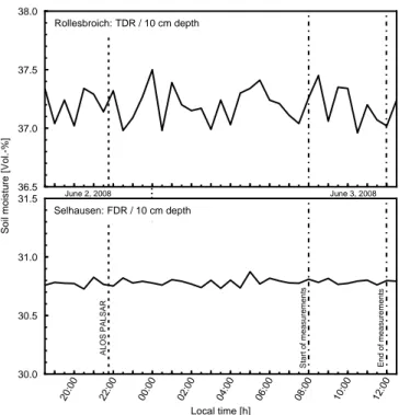
Supplementary Figure S2: Soil moisture at 10 cm below surface [ % (percentage of volumetric water content)] and soil temperature at 10 cm below surface (°C) over the Experiment

The objectives of this paper are: (i) to study the impact of soil moisture and temperature on the net ecosystem carbon balance and its components in two consecutive