A NALYSIS OF SURFACE SOIL MOISTURE
PATTERNS IN AN AGRICULTURAL LANDSCAPE UTILIZING MEASUREMENTS AND
ECOHYDROLOGICAL MODELING
Inaugural-Dissertation
zur
Erlangung des Doktorgrades
der Mathematisch-Naturwissenschaftlichen Fakultät der Universität zu Köln
vorgelegt von Wolfgang Korres
aus Bonn
2013
Berichterstatter: Prof. Dr. Karl Schneider
Prof. Dr. Georg Bareth
Tag der mündlichen Prüfung: 14.01.2013
Abstract
Soil moisture and its distribution in space and time plays a decisive role in terrestrial water and energy cycles. It controls the partitioning of precipitation into infiltration and runoff as well as the partitioning of solar radiation into latent and sensible heat flux. Therefore it has a strong impact on numerous processes, e.g., controlling floods, crop yield, erosion, and climate processes. Soil moisture, and surface soil moisture in particular, is highly variable in space and time and its spatial and temporal patterns in an agricultural landscape are affected by multiple natural (precipitation, soil, etc.) and agricultural (soil management, fertilization etc.) parameters. Against this background, the current study investigates the spatial and temporal patterns of surface soil moisture in an agricultural landscape, to determine the dominant parameters and the underlying processes controlling these patterns. The study was conducted on different spatial scales, from the field scale to the whole catchment scale of the river Rur (2364 km
2) in Western Germany, because observed patterns are intrinsically connected to the scale on which they are observed. For the investigation three different approaches were used:
Analysis based on A) Field measurements, B) Radar remote sensing, and C) Ecohydrological modeling. Extensive field measurements were carried out in a small arable land and grassland test site, measuring surface soil moisture, plant parameters, meteorological parameters, and soil parameters. These measurements were used to analyze the small scale (field scale) patterns of surface soil moisture and for the validation of the two other methods. Since large scale investigations based on field measurements are generally not feasible, surface soil moisture maps from radar remote sensing and ecohydrological modeling were used to analyze large scale patterns of surface soil moisture and their scaling properties.
Precipitation, vegetation patterns, topography and soil properties were found to be the dominant parameters for soil moisture patterns in an agriculturally used landscape.
Precipitation can be assumed to be homogeneous on the small scale, but can be very
heterogeneous on the large scale at the same time. Evapotranspiration causes high small scale
variability, especially during the growing season. If analyzed on coarser resolutions, this small
scale pattern is smoothed out. Topography is a source of small scale patterns only on wet
surface soil moisture states, because of the lateral redistribution of water during or shortly
moisture on all scales, due to the large heterogeneity of soil properties within a given soil type (small scale) and between different soil types (large scale). Altogether, the variability of surface soil moisture increases with an increasing size of the investigation area and with an increasing resolution within the investigation area. During the course of the year surface soil moisture variability and its scaling properties are being influenced by different parameters with temporally varying intensities. During the growing season, at the time of high small scale variability of evapotranspiration, the variability of surface soil moisture is high and decreases much stronger with decreasing spatial resolution of the investigation, than during times outside the growing season. In the beginning and towards the end of the year (outside the growing season, when the soil is wet) the patterns and their scaling properties are mainly determined by soil properties. Precipitation events generally superimpose their large scale patterns for a short period of time and diminish the small scale variability induced by evapotranspiration.
This thesis improves the knowledge about surface soil moisture patterns in agriculturally used areas and their underlying processes. The results of the scaling analysis indicate the potential to use vegetation and precipitation parameters for downscaling purposes.
Understanding the subscale soil moisture heterogeneity is, for example, particularly relevant
to better utilize coarse scale soil moisture data derived from SMOS (Soil Moisture and Ocean
Salinity) or the upcoming SMAP (Soil Moisture Active Passive) satellite measurements.
Kurzzusammenfassung
Bodenfeuchte und ihre räumliche und zeitliche Verteilung spielen eine entscheidende
Rolle im terrestrischen Wasser- und Energiekreislauf. Sie kontrolliert die Aufteilung von
Niederschlägen in Versickerung und Oberflächenabfluss und die Aufteilung von
Sonnenenergie in latenten und fühlbaren Wärmestrom. Dies begründet den unmittelbaren
Einfluss dieser Größe auf vielfältigste Prozesse, wie zum Beispiel auf Überflutungs- oder
Erosionsereignisse, auf Erntemengen oder klimatisch wichtige Größen wie zum Beispiel die
Lufttemperatur. Insbesondere die oberflächennahe Bodenfeuchte ist räumlich und zeitlich
sehr variabel und ihre Muster werden auf landwirtschaftlich genutzten Flächen von einer
Vielzahl natürlicher (z.B. Niederschlag, Bodeneigenschaften) und Bewirtschaftungsfaktoren
(z.B. Bodenbearbeitung, Saattermine, Erntetermine) bestimmt. Vor diesem Hintergrund
untersucht diese Studie die räumlichen und zeitlichen Muster der oberflächennahen
Bodenfeuchte auf landwirtschaftlich genutzten Flächen und analysiert die wichtigsten
Einflussfaktoren und zugrundeliegenden Prozesse, die diese Muster verursachen. Da ein
beobachtetes Muster immer direkt mit der Skala, auf der diese Beobachtung gemacht wurde,
verknüpft ist, wurde diese Studie auf verschiedenen räumlichen Skalen durchgeführt, die von
der Feldskala bis hin zur Skala des Gesamteinzugsgebiets der Rur mit einer Größe von
2364 km
2reicht. Für diese Arbeit wurden drei unterschiedliche methodische
Herangehensweisen verwendet: Analysen basierend auf A) Feldmessungen, B) Radar-
Fernerkundung und C) ökohydrologischer Modellierung. In einem ackerbaulich genutzten
Testgebiet und in einem Grünlandtestgebiet wurden umfangreiche Feldmessungen der
Bodenfeuchte, von Pflanzenparametern, von meteorologischen Parametern und
Bodenparametern durchgeführt. Diese wurden zur Analyse der oberflächennahen
Bodenfeuchtemuster auf der kleinen Skala (Feldgröße) und zur Validierung der beiden
weiteren Methoden verwendet. Da großflächige Untersuchungen auf der Basis von
Feldmessungen nicht durchführbar sind, wurden für die Untersuchung der
Bodenfeuchtemuster auf großen Skala und deren Skalierungseigenschaften
Bodenfeuchtekarten genutzt, die aus der Radar-Fernerkundung abgeleitet wurden oder aus der
ökohydrologischen Modellierung stammen.
Als Haupteinflussfaktoren für oberflächennahe Bodenfeuchtemuster in landwirtschaftlich genutzten Gebieten wurden Niederschlag, Landnutzung, Topographie und Boden ermittelt.
Niederschlag kann zwar auf der kleinen Skala als homogen angenommen werden, aber gleichzeitig große Heterogenität auf der großen Skala zeigen. Evapotranspiration im Zusammenhang mit kleinräumigen Landnutzungsmustern verursacht kleinräumige Variabilität, vor allem in der Hauptwachstumsperiode der Pflanzen. Mit einer Verkleinerung der Auflösung der Untersuchung werden diese kleinräumigen Muster durch Mittelung geglättet. Topographie verursacht ebenfalls kleinräumige Muster der Bodenfeuchte unter feuchten Bedingungen, da Wasser aus Niederschlagsereignissen lateral in tieferliegende Gebiete abgeleitet wird und dort zu einem Anstieg der Versickerung führen kann. Böden haben einen sehr großen Einfluss auf die Variabilität der Bodenfeuchte auf allen Skalen, da die Heterogenität der hydraulischen Bodeneigenschaften innerhalb eines Bodentyps auf der kleinen Skala ebenso groß sein kann wie zwischen unterschiedlichen Bodentypen auf der großen Skala. Insgesamt nimmt die Variabilität der oberflächennahen Bodenfeuchte mit der Vergrößerung der Auflösung der Untersuchung und der Größe des Untersuchungsgebietes zu.
Im Laufe eines Jahres verändern sich der Einfluss verschiedener Faktoren und deren Intensität auf die Muster und deren Skalierungsverhalten. Während der Hauptwachstumsperiode ist die durch die Evapotranspiration verursachte kleinräumige Variabilität sehr hoch, sinkt dann allerdings auch wesentlich schneller mit der Verringerung der Auflösung der Untersuchung als außerhalb der Hauptwachstumsperiode. In dieser Zeit, am Anfang und gegen Ende des Jahres, wenn der Boden feucht ist, bestimmen hauptsächlich Bodeneigenschaften das Muster und die Skalierung. Niederschlagsereignisse mit ihrem großskaligen Muster überlagern und dämpfen die durch die Evapotranspiration verursachte kleinskalige Heterogenität für einen kurzen Zeitraum.
Insgesamt verbesserte diese Arbeit das Verständnis von oberflächennahen
Bodenfeuchtemustern auf landwirtschaftlich genutzten Flächen und deren zugrundeliegenden
Prozessen. Die Ergebnisse der Skalierungsanalyse zeigen das Potenzial von Vegetations- und
Niederschlagsparametern zur Anwendung eines Downscaling-Verfahrens. Das Verständnis
der subskaligen Heterogenität von oberflächennaher Bodenfeuchte ist von besonderem
Interesse, um zum Beispiel großskalige aber gering aufgelöste Bodenfeuchtedaten aus SMOS
(Soil Moisture and Ocean Salinity) oder den kommenden SMAP (Soil Moisture Active
Passive) Satellitenmessungen besser nutzen zu können.
Acknowledgements
This thesis was prepared during the first phase of the Transregional Collaborative Research Center 32 (SFB/TR32) “Patterns in Soil-Vegetation-Atmosphere Systems:
Monitoring, Modeling, and Data Assimilation”, funded by the German Research Foundation (DFG). I gratefully acknowledge their financial support.
I wish to express my gratitude to my supervisor Prof. Dr. Karl Schneider for giving me the opportunity to work in his research group and in the SFB/TR32 project, for providing me with all essential background conditions that made this thesis possible and also for his guidance and invaluable suggestions for improving this work.
I also sincerely thank Prof. Dr. Georg Bareth for consenting to act as second examiner and Prof. Dr. Susanne Crewell for chairing the examination committee.
I am indebted to Prof. Dr. Peter Fiener, Dr. Tim Reichenau and Dr. Christian Koyama for many inspiring and fruitful discussions and collaborations.
I thank my colleagues within the research group for a stimulating and friendly working atmosphere: Dr. Verena Dlugoß, Dr. Christian Klar, Dr. Victoria Lenz-Wiedemann, Paul Wagner and Marius Schmidt.
Furthermore, I thank Sven Bremenfeld, Alexander Schlote, Florian Wilken and the many student helpers for their assistance during the field campaigns and the laboratory analyses.
Many thanks also go to the farmers in Rollesbroich and Selhausen for their permission to carry out our measurements on their fields.
I am grateful to all colleagues within the SFB/TR32 project for their friendly conversations and collaborations.
Last but not least, my heartfelt thanks to my family, my brother Martin, and especially my
Contents
Abstract ... III
Kurzzusammenfassung ... V
Acknowledgements ... VII
Contents ... VIII
1.
Introduction ... 1
1.1.
The importance of soil moisture in the soil-plant-atmosphere system ... 1
1.2.
Scope and outline of this thesis ... 2
2.
Soil moisture ... 5
2.1.
Definition of soil moisture ... 5
2.2.
Soil moisture measurements ... 5
2.2.1. Frequency Domain Reflectometry ... 8
2.2.2. Advanced Synthetic Aperture Radar ... 9
2.3.
Soil moisture modeling ... 9
2.4.
Patterns of surface soil moisture ... 11
3.
Analysis of surface soil moisture patterns based on field measurements ... 14
4.
Analysis of surface soil moisture patterns based on radar remote sensing ... 28
5.
Analysis of surface soil moisture patterns based on ecohydrological modeling ... 39
6.
Summary of results and conclusions ... 80
6.1.
Small scale surface soil moisture patterns ... 81
6.2.
Large scale surface soil moisture patterns ... 82
6.2.1. Validation of methods ... 82
6.2.2. Large scale patterns ... 83
6.3.
Scaling properties of surface soil moisture patterns ... 85
6.4.
General conclusions ... 86
6.5.
Outlook ... 87
References ... 89
1. Introduction
1.1. The importance of soil moisture in the soil-plant-atmosphere system
The water cycle is a key part of the global climate system. Water plays an important role in the Earth's energy budget, due to its high latent heat of fusion and vaporization. Only 0.0012 % of the global water and 0.035 % of the global fresh water (excluding Antarctica) is stored in soils (Oki and Kanae, 2006). Despite its seemingly negligible quantity when compared to global water resources, soil moisture is a key variable in hydrology, meteorology, and agriculture.
Soil moisture plays a central role in terrestrial water and energy cycles. Its distribution controls the partitioning of precipitation into infiltration and runoff (Western et al., 1999), hence it has a strong impact on the response of stream discharge to rainfall events, plays a significant role in producing floods (Kitanidis and Bras, 1980) and affects erosion processes from overland flow and the generation of gullies (Moore et al., 1988). Soil moisture controls the partitioning of incoming radiation into latent and sensible heat, due to its effects on evaporation and transpiration (Entekhabi and Rodriguez-Iturbe, 1994) and thus determines energy and mass fluxes in the soil-vegetation-atmosphere system.
Moreover, soil moisture enables and modulates plant growth and hence has a major
influence on crop yield and food production. Root zone soil moisture determines how much
water is available to plants for photosynthesis, which is regulated by their stomatal
conductance to water transfer. Through their roots, plants extract water from deeper soil
layers and reduce percolation of precipitation to the groundwater. The fact, that
evapotranspiration returns about 60 % of the land precipitation back to the atmosphere (Oki
and Kanae, 2006) and most of the evapotranspiration takes place through the stomata of plants
emphasizes the major importance of the feedback loop between soil moisture and plants in the
terrestrial water and energy cycles. Because of the influence on the partitioning of incoming
radiation into latent and sensible heat, soil moisture impacts on a variety of climate processes,
in particular air temperature, boundary layer stability and in some instances precipitation
(Seneviratne et al., 2010).
In addition, soil moisture plays a major role in the global carbon cycle (Falloon et al., 2011), since microbiological activity and the decomposition of soil organic matter are controlled by temperature and moisture conditions. It is also of great socio-economic interest.
Global population growth, rapid economic development and climate change intensify the demand of fresh water, e.g., for drinking, irrigation, and cooling (Arnell, 1999).
Consequently, information about the spatial and temporal patterns of soil moisture is a very important parameter in weather forecast and global climate models, due to the improved representation of interactive land surface processes, in predicting extreme events like droughts or floods, erosion modeling, water resource management, and agricultural applications, e.g., determination of sowing dates, rational irrigation practices, cultural practices or selective application of pesticides. However, soil moisture and surface soil moisture in particular, is highly variable in space and time, impacted by the heterogeneity of soil properties, topography, land cover, and meteorological conditions.
1.2. Scope and outline of this thesis
This thesis was embedded within the framework of the Transregional Collaborative Research Center 32 (SFB/TR32) with the title “Patterns in Soil-Vegetation-Atmosphere Systems: Monitoring, Modelling, and Data Assimilation” funded by the German Research Foundation (DFG). This multidisciplinary project involves research groups in the field of geophysics, soil and plant science, hydrology and meteorology located at the Universities of Aachen, Bonn, and Cologne and the Research Centre Jülich. The project aims at extending the knowledge about the origins of and the interrelations between spatial and temporal patterns within the soil-vegetation-atmosphere system and their relation to energy and matter. The research area is the Rur catchment in Western Germany. The research of our subproject within the SFB/TR32 focuses on the subject of surface soil moisture, an essential quantity in the context of the overall research of the SFB/TR32 project. This dissertation thesis aims at answering the following main research questions:
What are the dominant parameters and underlying processes for spatial and temporal patterns of surface soil moisture in an agriculturally used landscape?
How does the spatial variability of surface soil moisture change from the field scale to
the catchment scale?
How do surface soil moisture patterns and their scaling behavior change during the course of the year? What parameters determine the patterns and their scaling behavior at different times?
To address these main questions three different approaches were used: Analysis based on A) Field measurements, B) Radar remote sensing, and C) Ecohydrological modeling.
Extensive spatially distributed field measurements of surface soil moisture in a grassland and an arable land test site were conducted. To analyze the patterns and dominant parameters at the small catchment scale an Empirical Orthogonal Function (EOF) and a correlation analysis were used (see chapter 3). The measurements were also used to validate an empirical soil moisture retrieval algorithm for Advanced Synthetic Aperture Radar (ASAR) remote sensing data. Retrieved soil moisture data and the field measurements served as a basis for the analysis of statistical properties of surface soil moisture from the field scale to the whole catchment scale in terms of the relationship between soil moisture variability and mean soil moisture (see chapter 4). To identify and assess the influence of the main parameters and processes leading to the scale dependent variability of surface soil moisture, a process based, dynamic ecohydrological model was deployed and validated. The use of this model accounted for the complex interactions and feedbacks between soil, plant, and atmosphere. An autocorrelation and scaling analysis of the surface soil moisture data from different model runs was used to investigate the varying impact of soil, precipitation and vegetation on the autocorrelation structure and scaling properties of surface soil moisture patterns during the course of the year (see chapter 5).
This thesis is organized in the following manner:
This introduction (Chapter 1) is followed by a general chapter (Chapter 2), with definitions of the variable of interest (2.1), an introduction of soil moisture measurement methods (2.2), a short introduction of soil moisture modeling in the context of ecohydrology (2.3) and an integrated overview of the research on patterns of soil moisture (2.4). Chapters 3 to5 contain three research papers corresponding to the research approaches:
Chapter 3: Analysis of surface soil moisture patterns based on field measurements with the
paper title: “Analysis of surface soil moisture patterns in agricultural landscapes using
Empirical Orthogonal Functions”.
Chapter 4: Analysis of surface soil moisture patterns based on radar remote sensing with the paper title: “Variability of Surface Soil Moisture Observed from Multitemporal C-Band Synthetic Aperture Radar and Field Data”.
Chapter 5: Analysis of surface soil moisture patterns based on ecohydrological modeling with the paper title: “Patterns and scaling properties of surface soil moisture in an agricultural landscape: An ecohydrological modeling study”.
Chapter 6 summarizes the results and conclusions of this thesis regarding the small scale
patterns (6.1), the large scale patterns (6.2), and the scaling properties (6.3) of surface soil
moisture. Furthermore, in the general conclusions (6.4) the main research questions will be
addressed and a short outlook is given (6.5).
2. Soil moisture
2.1. Definition of soil moisture
Soil is a three phase system, consisting of soil particles, soil water, and soil air. The water contained in the unsaturated soil is defined as soil moisture (Hillel, 1998). The amount of water in the soil can be expressed in relative terms (volumetric soil moisture [m
3m
-3], gravimetric soil moisture [kg kg
-1] or saturation ratio) and in absolute terms (water depth [mm] or mass [kg]). The value of soil moisture is considered with regard to a given soil volume. This is highly relevant, when comparing different soil moisture measurements or estimations, because the considered volumes range from the top few centimeters of the soil (e.g., from radar remote sensing) or a small volume (e.g., from Frequency Domain Reflectometry measurements) to discrete soil layers (e.g., from modeling) or an extremely large volume (e.g., from Gravity Recovery and Climate Experiment, GRACE). For the definition of root zone soil moisture and total soil moisture the relevant soil volume will vary as a function of space and time, depending on the rooting depth of plants and the water table depth, respectively. Two other important quantities in hydrology and agricultural applications are field capacity and permanent wilting point. Above field capacity, water cannot be held against gravity and drains towards the groundwater table, and below wilting point the water is strongly bound to the soil matrix and not accessible to plants. The binding of the soil moisture to the soil matrix is characterized by the soil moisture potential. Field capacity and permanent wilting point are typically defined as corresponding to suction heads of pF 1.8-2.5, with pF being the logarithm of the cm of water column suction, and pF 4.2, respectively. These are approximated values, and the wilting point is depending on the vegetation type.
2.2. Soil moisture measurements
There are multiple techniques that are used to measure soil moisture. However, a method
to continuously measure the spatial patterns of soil moisture at larger scales is currently not
available. The available measurement methods can be differentiated in direct (measurement of
hydrological variable, e.g., rainfall depth) or indirect methods. Most soil moisture
measurement techniques employ indirect measurements methods, utilizing the measurements
of features which are closely linked to soil moisture (e.g. frequency modulation of an emitted signal for FDR measurements or electromagnetic emissions for remote sensing). These measurements are then converted by a rating function to a soil moisture value (Grayson and Blöschl, 2000). These conversions can introduce additional measurement errors. In the following section different methods of soil moisture measurement are introduced, however this short outline is not intended to be exhaustive.
The thermogravimetric method is a one of the few direct methods and determines the weight loss of a known volume of soil after oven drying at 105°C (Reynolds, 1970a). But it is a very time-consuming and destructive method, used for calibration and evaluation purposes.
Time and Frequency Domain Reflectometry (TDR, FDR) are used most often to investigate soil moisture at the point scale (Navarro et al., 2006; Roth et al., 1992). These techniques are based on the change of an emitted electromagnetic wave along some wave guides inserted in the soil depending on the dielectric constant of the wet soil (see 2.2.1). The sensors are either used on fixed locations to monitor temporal dynamics or as portable probes to study spatially distributed soil moisture patterns. To enlarge the number of measurement locations while simultaneously retain the high temporal resolution of the measurements, wireless sensor networks have been developed (Bogena et al., 2007), but they cannot be applied to surface soil moisture investigations in an arable land test site, due to the cultivation practices and the high effort of installation and deinstallation.
Geophysical methods like ground penetrating radar (GPR, Huisman et al., 2001),
electromagnetic induction (EMI, Sheets and Hendrickx, 1995) or electric resistivity
tomography (ERT, Kemna et al., 2002) make it possible to measure soil moisture in a less
invasive or even noninvasive way on larger areas, but they rely on highly detailed information
of subsurface properties and a site specific calibration. The GPR method uses the same
principle as TDR, only it uses a non-guided electromagnetic wave, measured between a
transmitter and a receiver. EMI measures the apparent electric conductivity of the soil,
depending on the water content of the soil, with a magnetic field. ERT measures the bulk soil
electric conductivity, related to the water content, between two or more electrodes inserted
into the soil. Other ground based methods are utilizing the sensitivity of cosmic ray neutrons
to water content changes to estimate surface soil moisture non-invasive for a spatial scale of
300 m radius around the measurement device (Zreda et al., 2008) or using fibre optic cables
(Sayde et al., 2010; Steele-Dunne et al., 2010) to estimate soil moisture along cables of over
10 km length, using the dependence of soil thermal properties on soil moisture, but with a
Remote sensing can be used to observe larger scale soil moisture patterns with different spatial and temporal resolutions. All remote sensing based approaches are indirect methods, measuring the color (at optical to mid-infrared wavelengths), parameters of the surface energy balance (e.g., temperature, at thermal infrared wavelengths) or dielectric properties (at microwave wavelengths) of the soil. For the retrieval of soil moisture the following microwave frequency bands are most important: L-band (wavelength 15 - 30 cm), C-band (3.8 - 7.5 cm) and X-band (2.5 - 3.8 cm). There are three types of remote sensing platforms, towers, aircrafts (airborne) and satellites (spaceborne), but for operational purposes spaceborne platforms are the prime choice, because of their global coverage and the regular nature of their overpasses (Wagner et al., 2007). Active radar systems measure the backscattering coefficient (reflectivity of the surface) of the emitted beam, whereas passive systems (Radiometers) measure the brightness temperature of the surface (product of emissivity and temperature). Active measurements are more sensitive to roughness and vegetation structure than passive measurements, but they provide a much better spatial resolution. Examples for Microwave radiometers (passive systems) are: Advanced Microwave Scanning Radiometer (AMSR-E) or Soil Moisture and Ocean Salinity (SMOS). Examples for Synthetic Aperture Radar (SAR, active systems) platforms are: RADARSAT-1, RADARSAT-2, ERS-1, ERS-2 and ENVISAT (all C-band) or JERS-1 and ALOS (L-band).
SAR systems allow monitoring patterns at higher spatial and lower temporal resolutions, while passive systems allow assessing patterns at lower spatial and higher temporal resolutions (Wagner et al., 2007).
In our study, we used FDR probes both for the spatial surface soil moisture measurements and the measurements of soil moisture time series on single locations. Moreover, we used data from the Advanced Synthetic Aperture Radar (ASAR) onboard the ENVIronmental SATellite (ENVISAT) launched by the European Space Agency (ESA). Therefore these techniques are described in the following sections 2.2.1 and 2.2.2. in more detail.
The organization of measurements can be characterized by three scales (spacing, extent,
and support) and has been termed “scale triplet” by Blöschl and Sivapalan (1995). The term
scale refers to a characteristic length or time scale. Spacing refers to the distance (or time)
between the measurements, extent to the overall coverage of the measurements (in time or
space), and support to the averaging volume or area (or time) of a single measurement. For
example, the FDR measurements in our grassland test site had 50 meter spacing (between the
measurements), 1000 meter extent (length of the test site), and 0.1 meter support (area
scale that is able to resolve all variability of the processes that influences the soil moisture patterns. If the spacing is too large, small scale variability will not be captured. If the extend is too small, large scale variability will not be captured and if the support is to large, variability will be smoothed out (Grayson and Blöschl, 2000). Thus, ideally the process scale equals the measurement scale (equals the model scale).
2.2.1. Frequency Domain Reflectometry
Frequency Domain Reflectometry (FDR) measurements (Navarro et al., 2006) are used in this study as a standard for in situ soil moisture measurements. The FDR probes (Delta-T Devices Ltd., Cambridge, UK) consist of a waterproof casing for the electronics and four 6 cm long parallel stainless steel rods (to be inserted into the soil) and a data logger. This system provides a quick and efficient method for measuring soil moisture patterns (with a handheld logging device) or soil moisture time series (with a stationary data logger). The soil moisture value is averaged over a sampling volume with about 6 cm in length (along the rods) and a diameter of approximately 10 cm.
FDR is an indirect method and it is based on the change of the amplitude of an emitted 100 MHz sinusoidal wave signal as a function of the soil dielectric constant, also known as permittivity or specific inductive capacity (Gaskin and Miller, 1996). The dielectric constant is a measure of how polarizable a material is, when subjected to an electric field and is measured usually in relation to the dielectric constant of free space (then called relative dielectric constant). The relative dielectric constant of soil consists of the relative dielectric properties of liquid water (approximately 80) and dry soil (2-5, depending on bulk density), and the volume fraction of each component involved. Thus, when the soil moisture content in the soil increases, the relative dielectric constant increases. However, the dielectric constant of moist soil is more complex than a simply weighted average of its components and the mixing model has many influencing factors (Jackson and Schmugge, 1989). A comprehensive overview over the topic complex dielectric constant is given by Von Hippel and Labounsky (1995). The most commonly used relationship to convert the dielectric constant to volumetric soil moisture is an empirical third order polynomial expression established by Topp et al.
(1980). This conversion is almost independent from soil density, soil texture, soil salinity and
soil temperatures (for temperatures between 10°C and 36°C) and has been used as a quasi-
standard method in various investigations.
2.2.2. Advanced Synthetic Aperture Radar
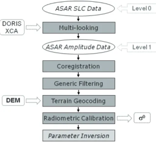
The Advanced Synthetic Aperture Radar (ASAR) was launched as one of ten instruments onboard the ENVISAT-1 satellite by the European Space Agency (ESA) with a sun- synchronous polar orbit in 2002. It is an active radar instrument, operating in C-band with a center frequency of 5.331 GHz (the corresponding wavelength is 5.62 cm) and can perform multiple acquisition modes. The penetration depth of the radar determines the sample volume and varies between half of the wavelength to the order of some tenths of the wavelength (in wet soil conditions). In our study wide swath images with a resolution of approximately 150 m and a swath width (width the sensor can observe) of 400 km were used, because this mode is suitable for the derivation of large scale surface soil moisture patterns. The single scenes were acquired on the same orbit, hence the time lag between the different images equals the orbital repeat cycle of the satellite of 35 days.
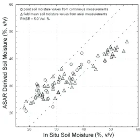
The derivation of surface soil moisture values from radar remote sensing is based on the sensitivity of the SAR backscatter intensity to the dielectric constant of the moist soil (see FDR measurements). But the backscatter signal at the C-band is also significantly influenced by vegetation and surface roughness, thus for the estimation of spatial soil moisture patterns, correction procedures for these two factors are required. Physically based backscatter models for the inversion of soil moisture from the radar data are only available for bare soil conditions and require either detailed independent soil data or additional radar data to isolate the effects of surface roughness and surface soil dielectric constant. This detailed additional data is often unavailable, particularly for larger areas. Empirical and semiempirical algorithms have shown their potential to derive soil moisture from single-frequency SAR data, but their applicability might be limited to the region where they are developed (Oh et al., 1992;
Rombach and Mauser, 1997). If transferred to a different area, they must be validated again.
An overview of the existing inversion approaches is given by Verhoest et al. (2008).
2.3. Soil moisture modeling
Soil moisture modeling in the context of ecohydrology can be characterized by two main
types of concepts: i) empirical modeling concepts, with only a statistical or conceptual (high
degree of abstraction) description of the processes and their underlying controlling factors and
ii) process based dynamic modeling concepts, with a process based description of the physical
processes and the capability of simulating nonlinear interactions. Process based dynamic
models are suitable for climate change studies, the analysis of complex cause and effect
principles and have a high transferability to other areas. The transferability of models or modeling concepts from the point or small scale, where they are being developed and validated, to the larger or even global scales is another big challenge and a large source of uncertainty. Three examples of concepts for bridging this scale gap are effective parameters (Hansen et al., 2007), Geo-complexes (Ludwig et al., 2003), and hydrological response units (HRUs, Flügel, 1995). Due to the large variety of models and model concepts with various complexities of process descriptions at different scales, a short description of the concepts in the model we used in our investigation is given in the following section instead of a general overview over different models and concepts (for this, see Pitman, 2003; Sellers et al., 1997).
The ecohydrological model used in this study is the DANUBIA simulation system. It is a component and raster based modeling tool designed for coupling models of different complexity and temporal resolution and consist of 17 components in its complete structure, representing natural as well as socio-economic processes (Barth et al., 2004; Barthel et al., 2012). It was developed in the GLOWA-Danube Project to investigate the impacts of Global Change on the Upper Danube catchment in Southern Germany. For the current study in the northern part of the Rur catchment, only the ecohydrological components regarding plant growth, soil nitrogen transformation, hydrology, and energy balance were used. These components model fluxes of water, energy, nitrogen and carbon in the soil-vegetation- atmosphere system using physically based process descriptions.
The vertical water fluxes in the soil are modeled using a modified Eagleson approach (Eagleson, 1978). The modification particularly pertains to describing water fluxes in soil by a user defined number of soil layers. Percolation of the upper soil layer is interpreted as effective precipitation for the downward layer (Mauser and Bach, 2009). Volumetric soil moisture and matrix potential is calculated according to the one-dimensional, concentration dependent diffusivity equation (Philip, 1960). Eagleson (1978) presented an analytical solution of the Philips equation for simplified boundary conditions to model the key processes of soil water movement, namely infiltration, exfiltration, percolation and capillary rise. Most of the hydrological models use a numerical solution of the Richards' equation to describe soil water flow (e.g. HYDRUS, Šimůnek et al., 2008), but for our distributed soil moisture modeling at larger scales only an analytical algorithm like the Eagleson approach is practical.
This analytical and physically based approach is computationally efficient and it avoids
iterative solutions. It has proven its applicability (Mauser and Bach, 2009; Schneider, 2003)
and all necessary input data can be derived from soil texture, which is extensively available
larger grid sizes comparable to our study (Vogel and Ippisch, 2008) and can in some cases lead to loss of the physical basis.
The crop growth model (Lenz-Wiedemann et al., 2010) simulates water, carbon, and nitrogen fluxes within the crops as well as the energy balance at leaf level. It models photosynthesis, respiration, soil layer-specific water and nitrogen uptake, dynamic allocation of carbon and nitrogen to four plant organs (root, stem, leaf, harvest organ), as well as phenological development and senescence. Resulting from the interplay of these processes, transpiration is a function of available energy, stomatal conductance (controlled by soil moisture and CO
2), and leaf area (emerging from carbon and nitrogen dynamics). The water and nitrogen uptake is differentiated between the different soil layers based on the distribution of the plant roots. The main concepts and algorithms are adopted and extended from the models GECROS (Yin and van Laar, 2005) and CERES (Jones and Kiniry, 1986). The soil nitrogen transformation model (Klar et al., 2008) is based on algorithms from the CERES maize model (Jones and Kiniry, 1986) and models nitrogen transformation processes:
Mineralization from two organic carbon pools (easily decomposable fresh organic matter and stable humus pool), immobilization, nitrification, denitrification, urea hydrolysis, and nitrate leaching. The iterative solution of the energy and mass balance is calculated based on the results exchanged between the soil component (including a soil temperature model from Muerth and Mauser, 2012) and the plant growth component. Meteorological input was derived from meteorological station data, using the method described by Mauser and Bach (2009).
The full coupling of the different components as well as the dynamic plant growth component (in contrast to a prescribed vegetation) consider the manifold interactions and feedbacks between soil, plant, and atmosphere with regard to water and energy fluxes and their resulting effect on soil moisture and evapotranspiration. Thus, DANUBIA is a suitable model to investigate soil moisture patterns at larger scales in strongly managed agricultural areas.
2.4. Patterns of surface soil moisture
Many factors control the spatial patterns and temporal dynamics of surface soil moisture.
Among these a distinction can be made between static and dynamic factors (Reynolds,
1970b). Static factors are particularly topography (e.g., slope and aspect affect runoff,
infiltration, and evapotranspiration) and soil properties (e.g., texture, porosity and organic
matter content affecting water holding capacity). Dynamic factors are meteorological conditions (e.g., precipitation, solar radiation, air temperature, wind speed, humidity), vegetation dynamics (e.g., influencing transpiration, evaporation from intercepted precipitation) and human management (e.g., irrigation). The influence of the different factors can vary significantly over time in the same landscape. Grayson et al. (1997) distinguish between two states: A) a wet state, denoted as non-locally controlled, which is dominated by lateral water movement through both surface and subsurface paths, with catchment terrain leading to organization of wet areas along drainage lines, and B) a dry state, denoted as locally controlled, dominated by vertical fluxes (e.g., evapotranspiration), with soil properties and only local terrain (areas of high convergence) influencing spatial patterns. But also precipitation as the main driver of surface soil moisture can occur at different scales in space and time. Convective precipitation can be characterized by small spatial extent, high intensities and short durations, with typical spatial scales of 1–10 km and typical temporal scales ranging from 1 minute to 1 hour. Whereas frontal weather systems tend to produce wide areas of relatively uniform rainfall with typical spatial scales of 100–1000 km and typical temporal scales of 1 day (Grayson and Blöschl, 2000).
Autocorrelation length is often used to analyze the spatial structure of soil moisture fields
and their driving parameters. For a small grassland catchment, Western and Grayson (1998)
found shorter autocorrelation lengths on wet days, related to the smaller spatial scale of lateral
redistribution, in contrast to longer autocorrelation lengths on dry dates, connected to the
larger scale of evapotranspiration as the dominant driver. At the field scale (mainly on wheat
fields) in a semi-arid climate, Green and Erskine (2004) found a spatial structure of surface
soil moisture, but no clear connection of the autocorrelation length to dry or wet soil moisture
conditions. Western et al. (2004) compared soil moisture autocorrelation lengths of soil
moisture and terrain attributes, indicating the important role of topography at one test site and
the variation of soil properties at other test sites. But these studies focused on small
catchments, mostly with homogeneous vegetation, therefore the influence of the interacting
factors topography, vegetation, soil, and precipitation on surface soil moisture patterns were
not investigated. Other studies used Empirical Orthogonal Functions to analyze the variability
of surface soil moisture and their driving factors over a large variety of scales, from the field
scale for agricultural sites (Yoo and Kim, 2004) to small catchment scales (Perry and
Niemann, 2007), and to regional scales (Jawson and Niemann, 2007). At the field and small
catchment scale topography related factors were found to be most important for the spatial
scale. This indicates that topographic characteristics influence soil moisture largely through lateral flows, which are not easily observed at larger scales.
Many studies have analyzed the statistical properties of the spatial structure of soil moisture in terms of the relationship between soil moisture variability and mean soil moisture using point measurements (e.g., Famiglietti et al., 1998; Western et al., 1998), remotely sensed images (e.g., Kim and Barros, 2002; Rodriguez-Iturbe et al., 1995) and model generated maps (e.g., Manfreda et al., 2007; Peters-Lidard et al., 2001). Contrasting findings of the relationship have been reported. Some studies found an increase of spatial variability with decreasing mean soil moisture (e.g., Choi and Jacobs, 2011; Famiglietti et al., 1999), others found opposite trends (e.g., Famiglietti et al., 1998; Western and Grayson, 1998) or were unable to detect a trend (e.g., Charpentier and Groffman, 1992; Hawley et al., 1983).
Teuling and Troch (2005) explained these contrasting findings by analyzing that both, soil properties and vegetation dynamics, can act to either create or destroy spatial variability. The main discriminating factor between both behaviors is a critical moisture content in the soil, defined by the transition between stressed and unstressed conditions for transpiration.
Moreover, Rodriguez-Iturbe et al. (1995) and Manfreda et al. (2007) showed that spatial soil
moisture variability is not only depending on mean soil moisture, but also varies with the
spatial scale of the analysis following a power-law relationship.
3. Analysis of surface soil moisture patterns based on field measurements
Journal article (published):
Korres, W., Koyama, C.N., Fiener, P., Schneider, K., 2010. Analysis of surface soil moisture patterns in agricultural landscapes using Empirical Orthogonal Functions. Hydrology and Earth System Science, 14(5): 751-764.
Permission to reprint:
The article and any associated published material is distributed under the Creative Commons
Attribution 3.0. Copyright on this article is retained by the authors. Original page numbers are
used.
www.hydrol-earth-syst-sci.net/14/751/2010/
doi:10.5194/hess-14-751-2010
© Author(s) 2010. CC Attribution 3.0 License.
Earth System Sciences
Analysis of surface soil moisture patterns in agricultural landscapes using Empirical Orthogonal Functions
W. Korres, C. N. Koyama, P. Fiener, and K. Schneider
Department of Geography, University of Cologne, Cologne, Germany
Received: 30 July 2009 – Published in Hydrol. Earth Syst. Sci. Discuss.: 24 August 2009 Revised: 3 April 2010 – Accepted: 14 April 2010 – Published: 12 May 2010
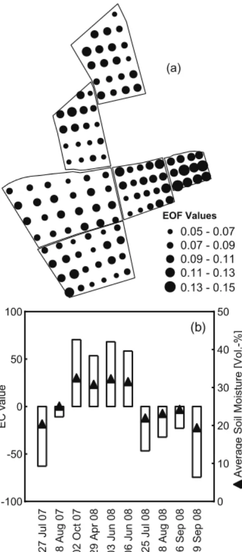
Abstract. Soil moisture is one of the fundamental variables in hydrology, meteorology and agriculture. Nevertheless, its spatio-temporal patterns in agriculturally used landscapes that are affected by multiple natural (rainfall, soil, topog- raphy etc.) and agronomic (fertilisation, soil management etc.) factors are often not well known. The aim of this study is to determine the dominant factors governing the spatio- temporal patterns of surface soil moisture in a grassland and an arable test site that are located within the Rur catchment in Western Germany. Surface soil moisture (0–6 cm) was mea- sured in an approx. 50×50 m grid during 14 and 17 measure- ment campaigns (May 2007 to November 2008) in both test sites. To analyse the spatio-temporal patterns of surface soil moisture, an Empirical Orthogonal Function (EOF) analysis was applied and the results were correlated with parameters derived from topography, soil, vegetation and land manage- ment to link the patterns to related factors and processes.
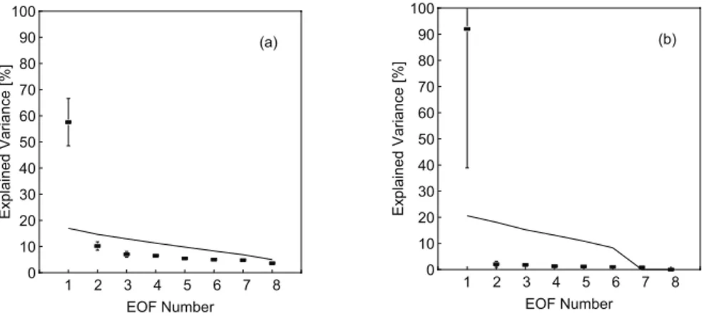
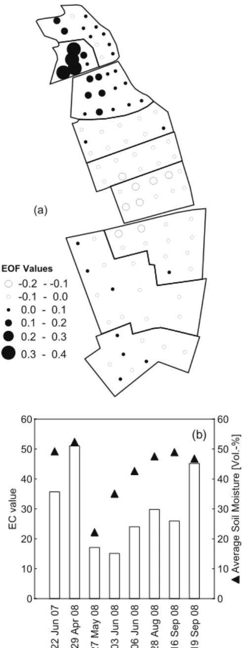
For the grassland test site, the analysis resulted in one sig- nificant spatial structure (first EOF), which explained 57.5%
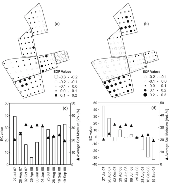
of the spatial variability connected to soil properties and to- pography. The statistical weight of the first spatial EOF is stronger on wet days. The highest temporal variability can be found in locations with a high percentage of soil organic carbon (SOC). For the arable test site, the analysis resulted in two significant spatial structures, the first EOF, which ex- plained 38.4% of the spatial variability, and showed a highly significant correlation to soil properties, namely soil texture and soil stone content. The second EOF, which explained 28.3% of the spatial variability, is linked to differences in land management. The soil moisture in the arable test site varied more strongly during dry and wet periods at locations
Correspondence to:W. Korres (wolfgang.korres@uni-koeln.de)
with low porosity. The method applied is capable of iden- tifying the dominant parameters controlling spatio-temporal patterns of surface soil moisture without being affected by single random processes, even in intensively managed agri- cultural areas.
1 Introduction
Soil moisture is one of the fundamental variables in hydrol- ogy, meteorology and agriculture as it plays a major role in partitioning energy, water and matter fluxes at the bound- ary between the atmosphere and the pedosphere. Its spatio- temporal distribution influences the partitioning of precipita- tion into infiltration and runoff (Western et al., 1999a) and it partitions the incoming radiation into latent and sensible heat due to the control of evaporation and transpiration. It has a strong impact on the response of stream discharge to rainfall events, it plays a significant role in producing floods (Kitani- dis and Bras, 1980) and affects erosion from overland flow and the generation of gullies (Moore et al., 1988). More dis- charge and erosion have been observed in areas with high soil moisture that are well connected to channels (Ntelekos et al., 2006). The spatio-temporal variation of soil moisture is also reflected in spatial patterns of plant growth and crop yield (Jaynes et al., 2003). For example, crop yield is highly sensitive to early season soil moisture conditions, especially during seed germination (Green and Erskine, 2004).
Due to difficulties in measuring spatio-temporal patterns of soil moisture at larger scales and owing to the impor- tance of these patterns for many environmental processes, great efforts were undertaken to derive spatially distributed soil moisture maps from remote sensing and modelling (Op- pelt et al., 1998; Owe and Van de Griend, 1998; Schneider,
2003). Since surface soil moisture data is potentially avail- able for large areas using remote sensing products (Koyama et al., 2010), it is of great interest to analyse the driving pa- rameters which explain these patterns. To build an adequate model, all relevant processes that affect spatial and temporal soil moisture variability must be identified and addressed. In case of strong spatial variations in soil properties or a dom- inance of vertical fluxes, such as evapotranspiration or infil- tration, soil moisture patterns are controlled by local prop- erties and processes (Grayson et al., 1997; Vachaud et al., 1985). If soil moisture is horizontally redistributed by lat- eral fluxes, non-local dependencies can play a decisive role (Herbst and Diekkr¨uger, 2003). Both, locally and non-locally controlled processes and their varying importance in time are essential for the determination of soil moisture patterns.
Hawley (1983) determined that topography (relative eleva- tion) is the most important driver of soil moisture in small agricultural watersheds. Even in watersheds with little slope, soil moisture values are consistently higher at the bottom of the slope. Vegetation tends to override this topographic influ- ence. The effect of soil texture on surface soil moisture ap- pears to be larger under wet conditions; minor variations in soil type seem to be insignificant. For all soil texture classes (except sands), soil moisture variability is typically high in a mid range between 18 and 23 Vol.-% (Vereecken et al., 2007). On a 1.4 ha hillslope, Burt and Butcher (1985) de- tected the development of saturated areas in downhill, low slope and convergent locations, indicating lateral redistri- bution of soil water via saturated flow above impermeable bedrock. The correlation between Wetness Index (WI; Beven and Kirkby, 1979) and soil moisture was generally better during wet conditions (Burt and Butcher, 1985). However, lateral water movement in unsaturated soils can also be ob- served and may reach the same order of magnitude as the vertical movement. This is caused by anisotropic permeabil- ity due to different soil layers (Zaslavsky and Sinai, 1981;
Herbst et al., 2006). For the Tarrawarra grassland catchment in south eastern Australia (Western et al., 1999a), the high- est correlation between soil moisture and topographic char- acteristics occurred for moderately wet conditions. This re- lationship deteriorates for dry and very wet (near saturation) conditions. The soil moisture autocorrelation calculated for different dates generally showed longer correlation length on dry dates, related to the larger spatial scale of evapotranspi- ration as the dominant driver. The shorter correlation length on wet days seems to be connected to the smaller spatial scale of lateral redistribution (Western et al., 1998). Green and Erskine (2004) found no clear correlation length of soil moisture at the field scale for a semi-arid climate. Western et al. (2004) compared soil moisture correlation lengths with the spatial correlation of terrain attributes indicating the im- portant role of topography at one site and the variation of soil properties at other sites. Empirical Orthogonal Func- tion (EOF) analysis can be used to identify the dominant processes and essential parameters controlling soil moisture
patterns. Since introduced to the analysis of geophysical fields by Lorenz (1956), EOF analysis has been widely ap- plied for the analysis of the spatial and temporal variability of large multidimensional datasets and has been commonly used in meteorological studies. More recently it has also been used to analyse soil moisture patterns at a large vari- ety of scales, from the field scale for agricultural sites (Yoo and Kim, 2004), to catchment scales (Perry and Niemann, 2007), and to regional scales (Jawson and Niemann, 2007;
Kim and Barros, 2002). The result of this analysis is a small number of spatial structures (EOFs) that explain a high per- centage of variation of the dataset and temporal varying co- efficients (ECs), which modulate the influence of these spa- tial structures in time. Utilizing correlation analyses, these underlying (stable) patterns of soil moisture variations can be connected to parameters derived from topography, soil, vegetation, land management and meteorology. Our dataset contains “snapshots” in time and the intention of our analysis is not to analyse continuous soil moisture seasonality. The main objectives of this study are to identify the dominant parameters and underlying processes controlling the stable spatial and temporal patterns of surface soil moisture under different soil moisture states and to examine whether the ap- plication of this method in agriculturally used areas, which are affected by heterogeneous, land-use dependent manage- ment procedures, also provides reasonable results.
2 Test sites
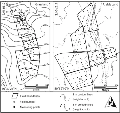
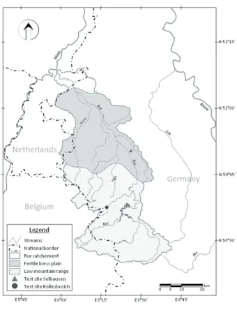
Field measurements were carried out in a grassland test site in Rollesbroich and an arable test site in Selhausen, both located west of Cologne, Germany. The grassland site (50◦3725N/6◦1816E) covers an area of approximately 20 ha with nine fields of extensively used grassland (Fig. 1).
This test site is typical for the low mountain ranges of the Eifel. Slopes range from 0 to 10◦, while altitude ranges from 474 to 518 m a.s.l. Mean annual air temperature and aver- age annual precipitation measured at a meteorological sta- tion 9 km west (altitude 505 m) of the test site are 7.7◦C and 1033 mm, respectively. No pronounced seasonality in precipitation can be found. The dominant soils are (gleyic) Cambisol, Stagnosol and Cambisol-Stagnosol. The grass- land vegetation is dominated by a ryegrass society, par- ticularly perennial ryegrass (Lolium perenne) and smooth meadow grass (Poa pratensis).
The arable site (50◦5210N/6◦274E) covers an area of approximately 34.3 ha and represents an intensively used agricultural area, where crops are grown on gentle slopes (0–
4◦). The altitude ranges from 102 to 110 m a.s.l. A mean annual air temperature of 9.8◦C and an average precipitation of 690 mm with slightly higher values occurring in June and July were measured at a meteorological station 4.5 km to the north-west (altitude 90 m). Main soils are (gleyic) Cambisol and (gleyic) Luvisol with a high amount of coarse alluvial
10 3
108 109
110 106
104 01
2 1 10
Field boundaries 1 m contour lines
(height a. s. l.) 5 m contour lines (height a. s. l.)
103505 515
510 515 5 50
500 490 495 5 48 47 480
5
0 51
50˚37'25''N
Measuring points
F1 F2
F3
F4 F5
F6
F7
F8
F9
F5
F6
F4 F2
F1
F3
Field number
F8
10 5
01 7
Grassland ArableLand
50˚52'10''N
0 150 300
Meters
6˚18'16''E 6˚27'04''E
0 150 300
Meters
Fig. 1.Topography, field layout and measuring grid of the grassland (Rollesbroich) and the arable test site (Selhausen).
deposits on a former river terrace in the eastern part. The land cover types during the measurement period were sugar beet (beta vulgaris), wheat (triticum aestivum), rye (secale cereale), oilseed radish (raphanus sativus oleiformes) and fallow.
3 Field measurements 3.1 Grassland test site
Surface soil moisture measurements for the topsoil layer (0–
6 cm) were performed on an approx. 50×50 m grid (Fig. 1).
The measurement locations were slightly adjusted according to local conditions such as field boundaries. While the aver- age distance to the next measurement location was 50 m, the minimum distance was 20 m and ranged up to 60 m. Mea- surements were taken during 14 campaigns from May 2007 to November 2008 at 41 to 96 locations. To provide represen- tative values, each measurement location is represented by the average of six measurements carried out within a radius of 10 cm. Soil moisture was measured with handheld FDR probes (Delta-T Devices Ltd., Cambridge, UK). The probes were calibrated individually in the laboratory using a mix- ture of water and glass beads to provide well defined water
content and tested on soil samples from the test sites. Based on these lab procedures, the FDR probes yield an absolute accuracy of±3 Vol.-% and a relative accuracy of±1 Vol.-%
(Delta-T Devices Ltd., Cambridge, UK). To investigate the influence of soil texture and soil organic carbon (SOC) on the surface soil moisture, soil samples in three depths (0–10 cm, 10–30 cm and 30–60 cm) were taken at every sampling lo- cation. Carbon content and soil texture were determined using mid-infrared-spectroscopy (Bornemann et al., 2008).
The results from spectroscopy analysis were calibrated to carbon content using samples analysed with a CN Elemen- tar Analysator (Elementar, Germany). In addition, topsoil (0–5 cm) porosity and soil organic matter (SOM) were mea- sured at four locations in the northern part of the test site, where very high surface soil moisture values (up to 75 Vol.-
%) were determined (especially field F2).
3.2 Arable test site
Similarly to the grassland test site, surface soil moisture (<6 cm) was measured in the arable test site on a grid of ap- prox. 50×50 m (Fig. 1). Again the locations were adjusted according to local conditions and field boundaries. Measure- ments were taken during 17 campaigns between May 2007 and November 2008 at 44 to 118 locations. Soil information
was taken from a high resolution soil map (Bodenkarte 1:50 000, Geologischer Dienst, North-Rhine-Westphalia). A terrace slope with an elevation difference of about 2–3 m cuts through the test site. Soil translocation by tillage operations at the edge of the terrace result in a high percentage of stones at the surface in the vicinity of the terrace slope. The up- per terrace plain has a high stone content, while the lower plain generally shows a lower stone content. The stone cover on the surface within a sample area of 0.4×0.4 m was vi- sually estimated at each measuring location using a wooden frame. On every location, three replicate measurements were taken. Using previously measured data of the course fraction of soil material, a relationship between the stone cover and the coarse fraction of the top soil layer (0–30 cm) was estab- lished by correlation analysis for two parallel transects with 8 measurement points. This analysis resulted in a Pearson correlation coefficient ofr=0.89. The stone cover analysis is subsequently used in the pattern analysis. The ground based data set was complemented by data on the tillage practice for each field.
4 Methods
4.1 Empirical Orthogonal Functions analysis
Empirical Orthogonal Functions (EOF) analysis is one of the best known data analysis techniques and a well established method of multivariate data analysis (Jolliffe, 2002). The EOF analysis, also known as principal component analysis, decomposes the observed variability of a dataset into a set of orthogonal spatial patterns (EOFs) and a set of time series called expansion coefficients (ECs). While single soil mois- ture patterns might be affected by random processes (e.g.
rainfall shortly before measuring), significant EOFs repre- sent stable patterns of a dataset and are by definition not ran- dom (definition of statistical significance in Sect. 4.2). The existing degree of randomness of a single soil moisture pat- tern is reflected by the associated EC, since the EC value represents the proportion of the significant EOF pattern in the soil moisture pattern of each date. In consequence, we did not use single soil moisture patterns (which might be random) but the EOF patterns for the subsequent correlation analysis.
Measurements, taken at locationxi(i=1,...p)and at time tj (j=1,. . .n), are arranged into a matrixD(nbyp:nsam- pling times andpsampling locations), in a so called S-mode.
Each row of the matrix represents the measurements at one point in time at all locations and each column represents a time series of measurements for a given location. To anal- yse the spatial variability of the data, a matrixFis computed from the matrixDby subtracting the average of each row of the data matrixD(average soil moisture for a given observa- tion time over all measurements locations). Analogously, to analyse the temporal variability, the average of each column
is subtracted from matrixD(average soil moisture for a given location for all measurements conducted at that location). In the next step, the covariance matrixR(pbyp) of the data matrixFis calculated:
R= 1
N−1FtF (1)
where the superscriptt indicates a transposed matrix andN is the number of observations.
Ris diagonalized to find the eigenvectors and eigenvalues:
RC=C (2)
where(pbyp) is a diagonal matrix containing the eigen- valuesλi ofR, andC(pbyp) contains the eigenvectorsci
ofRin the column vectors, corresponding to the eigenval- uesλi. For more details on the procedure see Jolliffe (2002);
Hannachi (2007) or Preisendorfer (1988).
This procedure rotates the original coordinate axes in a multidimensional space to align the data along a new set of orthogonal axes in the direction of the largest variance. Thus, the first axis or eigenvector is oriented in the direction that explains the largest variance. The subsequent axes are con- strained to be orthogonal to the axes computed before and consecutively explain the largest part due to the remaining covariance. The eigenvectorsci in the columns of the matrix Care the EOFs. The EOFs represent patterns or standing oscillations that are invariant in time. To analyse how the EOFs evolve in time, the expansion coefficients (ECs) asso- ciated with each EOF are calculated by projecting the matrix Fonto the matrixC:
A=FC (3)
where the matrixAcontains the expansion coefficientsai in the column vectors.
The EOF analysis produces p (p=sampling locations) EOF/EC pairs, but only min (n,p)eigenvalues (n=sampling times) are greater than zero and only a subset (usually a much smaller set) of these positive eigenvalues are meaningful. In general, the EOFs and ECs are rearranged in descending or- der due to their eigenvalues, so that the first EOF (EOF1) is associated with the largest eigenvalue. The fraction of vari- ance explained (EV) by each EOF can be found by dividing the associatedλi by the sum of all eigenvalues (the trace of ):
EVi= λi p i=1
λi
(4)
Following Bj¨ornsson and Venegas (1997) and Hannachi et al. (2007), the EOFs and the ECs can be determined very efficiently by singular value decomposition (SVD) without computing the covariance matrix and solving the eigenvalue problem. This decomposition by SVD provides a compact representation, because it drops unnecessary zero singular values (equivalent to zero eigenvalues).