Pathways of ice-wedge degradation in polygonal tundra under different hydrological conditions

(1)

https://doi.org/10.5194/tc-13-1089-2019

Pathways of ice-wedge degradation in polygonal tundra under different hydrological conditions

Jan Nitzbon^1,2,3, Moritz Langer^1,2, Sebastian Westermann³, Léo Martin³, Kjetil Schanke Aas³, and Julia Boike^1,2

1Alfred Wegener Institute, Helmholtz Centre for Polar and Marine Research, Telegrafenberg A45, 14473 Potsdam, Germany

2Geography Department, Humboldt-Universität zu Berlin, Unter den Linden 6, 10099 Berlin, Germany

3Department of Geosciences, University of Oslo, Sem Sælands vei 1, 0316 Oslo, Norway Correspondence:Jan Nitzbon (jan.nitzbon@awi.de)

Received: 28 September 2018 – Discussion started: 7 November 2018

Revised: 27 February 2019 – Accepted: 4 March 2019 – Published: 4 April 2019

Abstract. Ice-wedge polygons are common features of lowland tundra in the continuous permafrost zone and prone to rapid degradation through melting of ground ice.

There are many interrelated processes involved in ice-wedge thermokarst and it is a major challenge to quantify their influence on the stability of the permafrost underlying the landscape. In this study we used a numerical modelling approach to investigate the degradation of ice wedges with a focus on the influence of hydrological conditions. Our study area was Samoylov Island in the Lena River delta of northern Siberia, for which we had in situ measurements to evaluate the model. The tailored version of the CryoGrid 3 land surface model was capable of simulating the changing microtopography of polygonal tundra and also regarded lateral fluxes of heat, water, and snow. We demonstrated that the approach is capable of simulating ice-wedge degradation and the associated transition from a low-centred to a high- centred polygonal microtopography. The model simulations showed ice-wedge degradation under recent climatic conditions of the study area, irrespective of hydrological conditions. However, we found that wetter conditions lead to an earlier onset of degradation and cause more rapid ground subsidence. We set our findings in correspondence to observed types of ice-wedge polygons in the study area and hypothesized on remaining discrepancies between modelled and observed ice-wedge thermokarst activity. Our quantitative approach provides a valuable complement to previous, more qualitative and conceptual, descriptions of the possible pathways of ice-wedge polygon evolution. We concluded that our study is a blueprint for investigating thermokarst landforms and marks a step forward in understanding the

complex interrelationships between various processes shap- ing ice-rich permafrost landscapes.

1 Introduction

Many landscapes in the terrestrial Arctic are changing rapidly due to the thawing of ice-rich permafrost and subsequent ground subsidence, a process referred to as thermokarst (French, 2007; Rowland et al., 2010).

Thermokarst activity is apparent from various landforms including the formation of lakes, thaw slumps and thermo- erosional gullies (Kokelj and Jorgenson, 2013; Olefeldt et al., 2016). Another manifestation of thermokarst is the degradation of ice-wedge polygons, which is expressed by the formation of water-filled pits and troughs in polygonal tundra.

Advanced degradation of ice wedges can lead to a transition in the surface microtopography, from low-centred polygons to high-centred polygons (French, 2007). There is ev- idence from across almost all of the Arctic for increasing thermokarst activity in general (Kokelj and Jorgenson, 2013) and ice-wedge degradation in particular (Liljedahl et al., 2016) over the past few decades.

Ice-rich thermokarst landscapes are estimated to cover about 20 % of the Northern Hemisphere’s permafrost region but to store about half of the below-ground organic carbon of that region (Olefeldt et al., 2016). Because ice-wedge polygonal tundra is widespread in thermokarst landscapes it is of particular relevance to the local, regional, and possibly global cycling of energy, water, and carbon (Muster et al., 2012). The water and energy balances of polygonal tun-

(2)

dra are characterized by small-scale spatial heterogeneities (Langer et al., 2011b), which are influenced by the microtopography of the terrain. The degradation of ice wedges and concomitant microtopographic changes could therefore significantly alter water and energy fluxes in polygonal tundra (Liljedahl et al., 2016), with implications for a range of ecosystem functions such as, for example, the decomposition of organic matter (Lara et al., 2015). However, the implications of ice-wedge degradation for land–atmosphere and land–land energy, water, and carbon fluxes remain poorly constrained.

Ice-wedge degradation has been documented through in situ measurements at, and remote-sensing observations over, a number of different Arctic areas (Jorgenson et al., 2006;

Kokelj et al., 2014; Liljedahl et al., 2016; Fraser et al., 2018), and the biogeophysical processes controlling the evolution of ice-wedge polygons on different temporal scales have been described by conceptual models (Jorgenson et al., 2015; Kanevskiy et al., 2017). However, the prediction of thermokarst landscape evolution (as demanded by Rowland and Coon, 2015) requires numerical models capable of simulating the dominant processes associated with thermokarst landforms such as ice-wedge polygonal tundra (Painter et al., 2013). A variety of numerical modelling studies have ad- dressed different aspects of a broad range of biogeophysical processes associated with the evolution of ice-wedge polygons. Cresto Aleina et al. (2013) presented a data-driven, scalable approach to assessing the hydrological connectiv- ity of polygonal tundra and reported a non-linear hydrological control on methane fluxes. Several studies have noted the influence of microtopography and lateral fluxes on subsurface thermal and hydrological regimes, as well as on the biogeochemical processes in polygonal tundra areas (Kumar et al., 2016; Grant et al., 2017a, b; Bisht et al., 2018; Abolt et al., 2018). Liljedahl et al. (2016) investigated the hydrological implications of a transition from low-centred polygons to high-centred polygons and noted the important influence of spatially heterogeneous snow distribution. Abolt et al. (2017) investigated the ability of a hillslope diffusion approach to describe the geomorphological transition from low-centred polygons to high-centred polygons.

While all of these studies have improved our understanding of certain aspects of polygonal tundra systems, none used numerical models that could simulate the thermal and hydrological processes in polygonal tundra in combination with its dynamically changing microtopography due to melting of excess ground ice and successive ground subsidence (i.e.

thermokarst formation). Furthermore, most numerical models previously used to investigate ice-wedge polygons involved two- or three-dimensional fine-scale representations of the terrain, thereby significantly limiting the spatial features (a few metres across) and temporal periods (a few years) that could be simulated.

In this paper we present a modelling approach that is able to represent the landscape dynamics of polygonal tun-

dra, thereby taking into account transient microtopographic changes due to subsidence of ice-rich ground, as well as ac- counting for lateral fluxes of heat, water, and snow. Using a tiling approach to represent different parts of polygonal tundra allowed long-term (several decades) simulations on a landscape scale (several polygonal structures). We took ad- vantage of a detailed in situ data record from a site in the Lena River delta of northern Siberia (Boike et al., 2019), which was used to provide model parameters and meteorological forcing data, as well as for comparisons between actual measurements and the simulation results. Our main ob- jectives were

1. to demonstrate the ability of our tile-based modelling approach to simulate the process of ice-wedge degradation and the associated transition from low-centred polygons to high-centred polygons.

2. to assess the stability and the evolution of ice wedges in the study area under present-day climatic conditions but different site-specific hydrological conditions.

3. to quantify the implications of ice-wedge degradation for land–atmosphere and lateral (land-land) water and energy fluxes.

For this we performed and analysed numerical simulations, using a tailored version of the CryoGrid 3 land surface model (Westermann et al., 2016). Our investigations aimed at understanding the evolution of ice wedges in polygonal tundra in equilibrium with the recent climatic conditions, while we did not address projections of ice-wedge development in a changing future climate.

2 Methods 2.1 Study area

Our study area was Samoylov Island in the Lena River delta, northern Siberia (72.36972^◦N, 126.47500^◦E), which lies within the lowland tundra vegetation zone and is un- derlain by continuous permafrost. The climate on the island is Arctic continental with a mean annual air temperature (MAAT) below −12^◦C, minimum temperatures below−45^◦C, and maximum temperatures above 25^◦C (Boike et al., 2013, 2019). The average annual liquid precipitation is approximately 169 mm. There is typically continuous snow cover from the end of September to the end of May, with a mean end-of-winter thickness of about 0.3 m; the remaining months are mostly snow-free. The permafrost in the Lena River delta extends to depths of between 400 and 600 m (Yer- shov et al., 1999) with ground temperatures (in 2006) at a depth of 27 m of about−9^◦C (2006) (Boike et al., 2019).

(3)

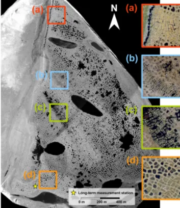
Samoylov Island belongs to the first river terrace of the Lena River delta, which was formed by fluvial erosion and sedimentation during the Holocene. The sediments in the upper soil layers have a silty to sandy texture with variable mineral (20 %–40 % by volume) and organic contents (5 %–10 % by volume) (Boike et al., 2013). Peat layers of variable thickness with higher organic contents have accu- mulated at the surface. These Holocene deposits are super- saturated with ice, with an average volumetric ice content of at least 60 %–70 % (Zubrzycki et al., 2013). The spatial distribution of ground ice is highly variable due to the pres- ence of ice wedges underlying most of the island. The pres- ence of ice wedges is expressed at the ground surface by a polygonal-patterned landscape, formed as a result of repeated frost-cracking of the ground and subsequent infiltration and freezing of water. Apart from a few large thermokarst lakes, Samoylov Island is largely covered by ice-wedge polygons whose surface features vary greatly across the island (Fig. 1).

Some areas are covered with un-degraded low-centred polygons (LCPs; Fig. 1d), while initial degradation features, as described by Liljedahl et al. (2016) and Kanevskiy et al.

(2017), are visible in other parts of the island (Fig. 1b).

Due to advanced degradation of ice wedges, some polygons feature a reversed, high-centred relief (high-centred polygons: HCPs) and interconnected troughs that can be either dry or water-filled (Fig. 1a and c). The polygonal tundra on Samoylov Island has been previously investigated in a number of studies, with a particular focus on measuring its water and energy balances (Boike et al., 2008; Langer et al., 2011a, b; Helbig et al., 2013). Moisture levels on the island are spatially variable with a high abundance of polygonal ponds and a few larger water bodies in its central part and dryer, well- drained areas towards the margins of the island (Muster et al., 2012).

The diversity of ice-wedge polygons that evolved under identical climatic conditions on Samoylov Island makes it a highly suitable location for studying the factors affecting the evolution of polygonal tundra. The long-term monitoring of meteorological and ground conditions (Boike et al., 2013, 2019) also provides valuable in situ baseline data (see Fig. 1 for the location of long-term measurement station).

These data have been used as input for permafrost models in a number of modelling studies (Westermann et al., 2016, 2017; Langer et al., 2016; Gouttevin et al., 2018), as well as for their validation.

2.2 Model description

2.2.1 Tile-based representation of polygonal tundra The subgrid-scale heterogeneity of land surfaces (e.g. with regard to vegetation or snow cover) has previously been taken into account in LSMs using tiling approaches (Avis- sar and Pielke, 1989; Koster and Suarez, 1992; Aas et al., 2017). In this study we have used a similar approach to repre-

Figure 1. Aerial image of Samoylov Island with enlargements showing various types of ice-wedge polygons in different parts of the island, all of which evolved under identical climatic conditions:(a)high-centred polygons with drained troughs;(b)water- filled troughs that are indicative of initial ice-wedge degradation;

(c)high-centred polygons with water-filled troughs;(d)low-centred polygons with wet or water-covered centres. The central part of the island is relatively wet and contains a large number of water bodies, while the surrounding areas are drier and in part drain into the surrounding river delta. The location of the long-term measurement station for soil and meteorological conditions described in Boike et al. (2019) is indicated by a yellow star.

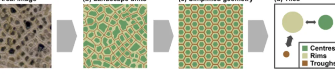
sent the spatial heterogeneity of permafrost landscapes, with each landscape tile representing a distinct part of the polygonal tundra (Fig. 2a). We subdivided the polygonal patterned landscape into three landscape units according to what we refer to as its microtopography: polygon centres (C), elevated rims (R), and a network of troughs (T) that spreads among the distinct polygonal structures (Fig. 2b). A similar partitioning of polygonal tundra has been used previously (Muster et al., 2012; Kumar et al., 2016; Grant et al., 2017a, b). Each of these landscape units constitutes a certainareal fractionγ of the overall landscape. We further simplified the partitioned landscape by assuming that it was made up of equally sized hexagons arranged on a regular grid (Fig. 2c). This assumption allowed us to derive topological relationships among the different landscape units, in particular lateraldistances D and contact lengthsL (see Appendix C for details and equations). Each of the landscape units (C, R, and T) was in- tegrated into a single representative tile (Fig. 2d). The land-

(4)

Figure 2.In our model framework the spatial heterogeneity of polygonal tundra microtopography is represented by three landscape tiles (polygon centres, C; polygon rims, R; troughs, T). The assumption of equally sized hexagons arranged on a regular grid makes it possible to quantify lateral transport processes among the tiles.

scape tiles were coupled by lateral transport processes whose magnitudes were determined by the topological relationships among the relevant tiles (Sect. 2.2.4). Note that apart from the partitioning into centres, rims, and troughs, our approach did not take into account topographic features of individual polygons. Instead, we assumed that larger areas with multiple polygons of similar topography and subject to similar hydrological conditions can be described via a single “effective”

polygon composed of the three tiles.

In order to reflect microtopographic differences within the polygonal tundra landscape, each tile was associated with a particular surface altitude (a).¹We defined three types of ice- wedge polygonal tundra based on the soil surface altitudes of the tiles. We designated the state in which the centre tile had the lowest elevation as low-centred polygonal tundra (LCP):

LCP: aC≤min(aR, aT) . (1)

Initial ice-wedge degradation is typically characterized by subsidence of the soil surface within the troughs. Those configurations in which the troughs subsided below the level of the centre but with the rims remaining elevated relative to the centre were designated intermediate-centred polygonal tundra (ICP):

ICP: aT< aC< aR. (2)

Finally, configurations in which the centre tile had the highest elevation were designated high-centred polygonal tundra (HCP):

HCP: aC≥max(aR, aT) . (3)

These definitions of polygonal tundra microtopography (LCP→ICP→HCP) correspond approximately to the three stages of ice-wedge degradation qualitatively depicted by Liljedahl et al. (2016) in their Fig. 1c and to the definitions of polygon types by MacKay (2000).²

1Throughout this paper we used the term altitude (a) when referring to the height above sea level and the term elevation (e) when referring to the height above the initial position of the centre tile (a_C), which serves as a reference height.

2Note that we excluded the caseaR< a_C< aTfrom these definitions as it corresponds to a state that is not observed in nature.

2.2.2 CryoGrid 3 Xice land surface model

To simulate the ground thermal regime of polygonal tundra, we used a parallelized version of the CryoGrid 3 land surface model in which each of the tiles described in Sect. 2.2.1 (C, R, and T) was assigned a one-dimensional representation of the subsurface (see Westermann et al., 2016, for a detailed description, and Nitzbon et al., 2019a, for the model source code). The numerical model simulates the temporal evolution of the ground temperature profile (T (z)) by solving the one- dimensional heat conduction equation, taking into account the phase change of water through an effective heat capacity:

C(z, T )+ρwLsl

∂θ_w

∂T ∂T

∂t = ∂

∂z

k(z, T )∂T

∂z

, (4)

whereθw is the volumetric water content,ρwthe density of water, andLslthe latent heat of fusion of water. The thermal properties of the soil cells (volumetric heat capacityC(z, T ) and thermal conductivityk(z, T )) are derived from the volumetric fractions of mineral, organic, water, ice, and air (see Westermann et al., 2013, for details). The lower boundary condition is prescribed by a constant geothermal heat flux (Q_geo), while the boundary condition at the surface is given by the ground heat flux (Q_g), which is obtained by explic- itly solving the surface energy balance (SEB) equations from the meteorological forcing data. The model further simulates the build-up and ablation of the snowpack, heat conduction within the snow, and water infiltration and refreezing within the snowpack. CryoGrid 3 uses a first-order forward Euler algorithm with adaptive time step for the numerical integration of the heat conduction equation.

The unique feature of CryoGrid 3 that enables it to simulate the evolution of ice-wedge polygons is its excess ground ice scheme (“Xice”), which uses a simple parameterization for excess ice melt and the resulting ground subsidence and water body formation, based on an algorithm proposed by Lee et al. (2014). This involves each cell of the discrete one- dimensional grid that represents the subsurface in the model being assigned a “natural” porosity (φ_nat). Frozen grid cells for which the volumetric water content (θ_w) exceedsφ_natare considered to contain excess ice. Once a grid cell containing excess ice thaws, the excess water (θ_w−φ_nat) is routed upwards while the solid soil matrix material of the cells above is

(5)

routed downwards such that it occupies the natural volumetric matrix fraction (1−φnat). Continued thawing of excess ice cells results in a net subsidence of the soil surface and potentially in the formation of a water body at the surface, depending on the treatment of excess water.

2.2.3 Hydrology scheme for unfrozen ground

To simulate the subsurface hydrological regime of the active layer we enhanced CryoGrid 3 with a hydrology scheme for unfrozen ground conditions. We used an instantaneous infiltration scheme which assumes rapid vertical water flow compared to the rates of other processes represented in the model. This is a valid assumption for the upper soil layers of tundra wetlands, which are typically characterized by large hydraulic conductivities (Boike et al., 2008) and in which infiltration into the active layer is mainly controlled by thaw depth (Zhang et al., 2010).

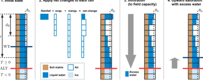
Given the preconditions of a snow-free and unfrozen soil surface, the hydrology scheme simulates the change in water content (θ_w) of each grid cell (within the soil domain and water bodies atop the soil surface) resulting from precipitation, evapotranspiration, and infiltration (Fig. 3). Wa- ter gained from rainfall (and snowmelt) is added to the uppermost soil grid cell. Reductions in soil water content due to evaporation and transpiration are distributed down to a characteristic evaporation depth (dE) and root depth (dT). An infiltration algorithm is then used to take into account the changes in water content due to precipitation and evapotranspiration; this first routes water downwards to the bottom of the active layer, setting the soil water content of all grid cells at maximum to the field capacity (θ_fc). Potential excess water is then pooled upwards by successively saturating the grid cells, which leads to the formation of a water table within the active layer (or even above the soil surface). Note that no sensible heat is transported with the infiltrating water; i.e. the process of heat advection is not taken into account by Cryo- Grid 3. A quantitative description of the hydrology scheme is given in Appendix A.

We note that the employed hydrology scheme is rather simplistic compared to other schemes available (e.g. Painter et al., 2016). We confirmed, however, that the employed scheme, in combination with the lateral water transport scheme detailed in Sect. 2.2.4, was sufficiently suited to reflect the spatial heterogeneity of the subsurface hydrological regime of polygonal tundra (see Sect. 3).

2.2.4 Lateral transport of heat, water, and snow among tiles

We further enhanced CryoGrid 3 by taking into account lateral subsurface heat and water fluxes among the landscape tiles, as well as snow redistribution. Topological characteristics of and relationships among the tiles (areaA, thermal

distanceD^th, hydraulic distanceD^hy, contact lengthL) were used to quantify the magnitudes of the lateral fluxes.

Lateral transport of heat. The lateral heat flux between adjacent tiles is computed for each cell of the vertically dis- cretized grid of all tiles, according to Fourier’s law. The heat flux q_α,i^th (J s⁻¹) to the cell with index i of tile α from all adjacent tiles is given as

q_α,i^th = X

β∈N(α)

k_αβⁱ T_βⁱ−T_αⁱ

D^th_αβ L_αβ1ⁱ_α, (5) whereN(α) denotes all tiles adjacent to α, kⁱ_αβ is the effective lateral thermal conductivity (Eq. B1 in Appendix B), Tⁱ refers to the temperature, and 1ⁱ refers to the height of grid celli. The lateral heat fluxes are added after each lateral transport time step1t_latto the vertical heat fluxes resulting from heat conduction and boundary fluxes (i.e. geothermal and ground heat fluxes).

Lateral transport of water between tiles. Lateral water fluxes between adjacent tiles are calculated as bulk fluxes, based on Darcy’s law. Given the precondition of a snow-free and unfrozen land surface, the lateral water fluxq_α^hy(m s⁻¹) to tileαfrom all adjacent tiles is given as

q_α^hy= X

β∈N(α)

K_αβwβ−max(wα, fα) D^hy_αβ

HαβLαβ

A_α , (6)

whereK_αβ is the saturated hydraulic conductivity between tilesαandβ,w_α the elevation of the water table of tileα, andf_α the elevation of the frost table (i.e. the bottom of the active layer) of tile α.H_αβ is the hydraulic contact height between tilesαandβ, which is obtained as follows:

H_αβ=min

w_β−max(w_α, f_α) , w_β−f_β

. (7)

The bulk lateral fluxesq_α^hy are applied to each tileα after each lateral transport time step1t_latusing the instantaneous infiltration scheme described in Sect. 2.2.3. Note that a tile for which no water table forms above the frost table can only receive lateral water fluxes. To ensure conservation of water, lateral fluxes are proportionally reduced if insufficient water is available in those tiles that “lose” water.

Exchange of water with the surrounding terrain. The trough tile is hydrologically connected to a theoretical external “water reservoir” that has a constant water level (w_res).³ This water level serves as a hydrological boundary condition between the modelled polygonal tundra and the surrounding terrain. A low water level in the external water reservoir leads to drainage of the troughs while a high water level results in their inundation. The lateral water fluxes from the reservoir

3Note that we used the symboleres when the reservoir water level is given relative to the initial altitude of the centre tile (e_res= wres−a_C).

(6)

Figure 3.Schematic illustration of the hydrology scheme for unfrozen ground conditions. The net changes due to precipitation and evapotranspiration are calculated during each time step of the model. The instantaneous infiltration routine involves downwards routing of water to the bottom of the active layer (ALT) and saturation with excess water from the bottom upwards. The water table (WT) forms above the uppermost water-saturated grid cell. Details on the hydrology scheme are given in Appendix A.

to the troughs (q_res^hy) are calculated in a similar way to those in Eq. (6), as follows:

qres^hy=Kres

w_res−max

w_T, f_T2

A_T , (8)

whereK_resis the reservoir hydraulic conductivity that, compared to the saturated hydraulic conductivity K, also in- corporates the topological parameters for hydraulic distance (D^hy) and contact length (L) between the reservoir and the trough tile.

Lateral transport of snow.Snow redistribution due to wind drift is assumed to occur among all tiles. A terrain index (I_α) that depends on the difference of the snow surface elevation (a_α) and the mean surface elevation (a) is calculated and indicates whether tileαloses or gains snow due to snow redistribution. The mobile snow of the more elevated tiles is redis- tributed amongst the less elevated tiles while at the same time taking into account the conservation of mass, leading to a levelling out of the snow surfaces, The “snow catch” effect of vegetation is taken into account by treating only snow above a threshold height (h^catch_α ) as “mobile” snow. Furthermore, lateral snow transport does not occur during melting conditions, i.e. if any snow cell has a positive temperature (Tⁱ>0) or contains liquid water. The governing equations of the lateral snow transport scheme are provided in Appendix B.

2.3 Model setup and simulations 2.3.1 Topology

As described in Sect. 2.2.1, we represented the spatial heterogeneity of the polygonal tundra landscape using three tiles (C, R, and T) and a theoretical, external water reservoir (de-

noted with subscript “res”). Figure 4 provides a schematic representation of the lateral connections among these tiles and indicates important parameters used to characterize the topology and microtopography in the model setup. Polygon centres are adjacent only to the rims, while the rims are also connected to the troughs. The troughs are hydrologically connected to the external water reservoir, which makes it possible to exchange water with the surrounding terrain (Fig. 4). We derived the topological relationships among the tiles (areas, contact lengths, and distances) based on an assumed regular hexagonal grid (see Fig. 2c). We estimated the areal fraction (γ) of the tiles (Table 1) on the basis of land cover classifications for Samoylov Island by Muster et al. (2012). The contact lengths (L_αβ), thermal distances (D^th), and hydraulic distances (D^hy) between adjacent tiles were calculated on the basis of geometric assumptions (i.e.

regular hexagonal grid) and the mean size of polygons on Samoylov Island given by Muster et al. (2012) (see Fig. 4 and Appendix C for details).

2.3.2 Microtopography

The lateral fluxes of snow, water, and heat are also influenced by the microtopography of the terrain, which is reflected in the different relative elevations of the tiles. We assumed that the initial elevation of the rims (e_R) of intact low-centred polygons relative to the centres was 0.4 m (Boike et al., 2019) and that the troughs were initially 0.1 m lower than the polygon rims (Table 1). The water level in the external water reservoir relative to the initial altitude of the polygon centres (e_res) was varied among different runs. In order to take into account variability in the polygon topology and micro-

(7)

Table 1.Parameters used to specify the topology and the microtopography for the tile-based model of polygonal tundra. Note that the initial altitude of the tiles can change due to ground subsidence. Lateral distances and contact lengths are calculated from these values using the formulas in Appendix C.

Parameter Symbol Unit Centre Rim Trough Total Reference

Altitude (initial) a m 20 20.4 20.3 – Boike et al. (2013)

Area Atot m² – – – 140 Muster et al. (2012)

Areal fraction γ – 0.3 0.6 0.1 1 Muster et al. (2012), Langer et al. (2011b)

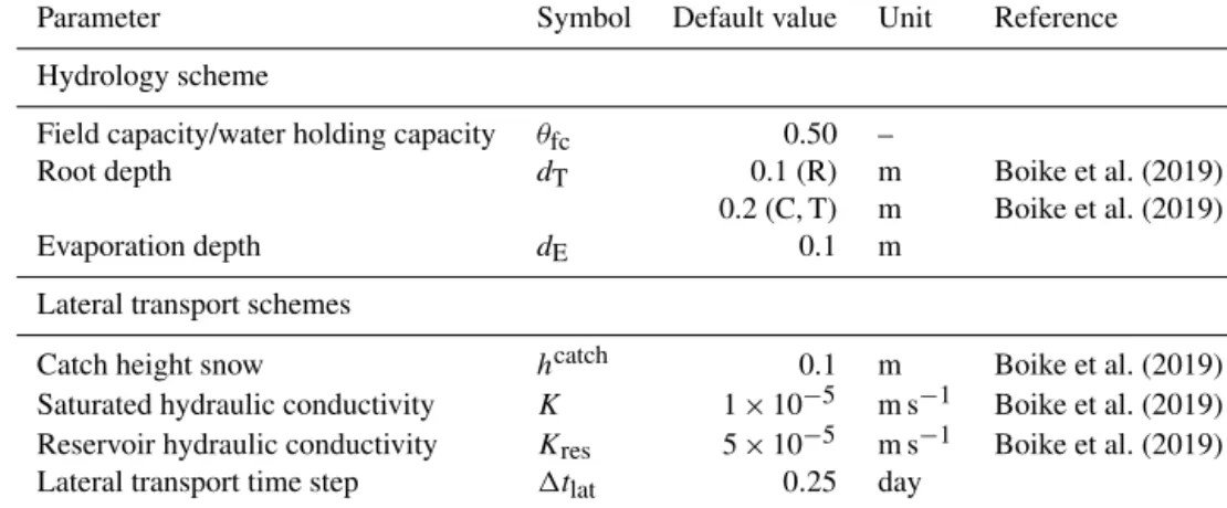
Table 2.New parameters introduced with the hydrology scheme and the lateral transport schemes described in this paper.

Parameter Symbol Default value Unit Reference

Hydrology scheme

Field capacity/water holding capacity θ_fc 0.50 –

Root depth d_T 0.1 (R) m Boike et al. (2019)

0.2 (C, T) m Boike et al. (2019)

Evaporation depth d_E 0.1 m

Lateral transport schemes

Catch height snow h^catch 0.1 m Boike et al. (2019)

Saturated hydraulic conductivity K 1×10⁻⁵ m s⁻¹ Boike et al. (2019) Reservoir hydraulic conductivity K_res 5×10⁻⁵ m s⁻¹ Boike et al. (2019)

Lateral transport time step 1t_lat 0.25 day

Figure 4.Setup of the coupled tiles (centres, C; rims, R; troughs, T) with parameters specifying the topology (reflected by areal fractions,γ; hydrological distances,D^hy; and thermal distances,D^th) and microtopography (reflected by elevations,e, relative to the altitude of the centre tile,a_C) of the polygonal tundra landscape. Each tile was assigned a one-dimensional representation of the subsurface, for which a parallelized version of the CryoGrid 3 land surface model was used. Water can also be exchanged with the surrounding terrain, which is represented by a theoretical water reservoir (res) with a fixed water level (eres) and a hydraulic conductivity (Kres).

Subscripts denote the tile(s) the parameters are relating to.

topography we conducted a sensitivity test and compared the modelled results with in situ measurements (see Sect. 3).

2.3.3 Parameters

Many of our model parameters were adopted from previous studies of the same study area that also used CryoGrid 3 (see

Table D1 in Appendix D). The parameters introduced with the hydrology scheme (Sect. 2.2.3) and the lateral transport scheme (Sect. 2.2.4) are summarized in Table 2, which also includes the default values and ranges assumed in this study.

We assumed a field capacity for the upper soil layers (θ_fc) of 0.50, which is in agreement with typical volumetric water contents in unsaturated soil layers, measured during the summer (Boike et al., 2019, Table 1). The root depth (dT) was set to 0.2 m for the polygon centres and troughs, which are typically covered with mosses and sedges, and to 0.1 m for the rims, where the mosses have shallower roots. The evaporation depth (dE) was set uniformly to 0.1 m for all tiles.

The saturated soil hydraulic conductivity (K) among all connected tiles was set to 1×10⁻⁵m s⁻¹and the reservoir hydraulic conductivity (K_res) was set to 5×10⁻⁵m s⁻¹; both values were of the same order of magnitude as the various estimates for the uppermost soil layers in the same study area (1.09–46.3×10⁻⁵m s⁻¹; Boike et al., 2019). The lateral transport schemes were run in intervals of 6 h (1t_lat= 0.25 day). Those parameters for which no published values were available have been estimated by the authors who have long-time field experience in the study area.

2.3.4 Soil stratigraphies

The soil stratigraphies were based on the stratigraphy provided in Westermann et al. (2016) for a polygon centre on Samoylov Island. However, we modified the stratigraphies for the different tiles to reflect the spatially heterogeneous

(8)

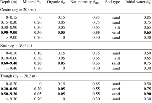
Table 3.Overview of the soil stratigraphies used for polygon centres, rims, and troughs. Excess ice layers (θ_w⁰> φnat) are shown in bold.

Depths are relative to the initial altitude (a) of the respective tile.

Depth (m) Mineralθm Organicθo Nat. porosityφnat Soil type Initial waterθ_w⁰ Centre (a_C=20.0 m)

0–0.15 0 0.15 0.85 sand 0.85

0.15–0.30 0.20 0.05 0.75 sand 0.75

0.30–0.90 0.30 0.05 0.65 silt 0.65

0.90–9.00 0.30 0.05 0.55 sand 0.65

>9.00 0.70 0 0.30 sand 0.30

Rim (a_R=20.4 m)

0–0.10 0.10 0.15 0.75 sand 0.50

0.10–0.60 0.30 0.05 0.65 silt 0.65

0.60–9.40 0.20 0.05 0.55 sand 0.75

>9.40 0.70 0 0.30 sand 0.30

Trough (a_T=20.3 m)

0–0.20 0 0.15 0.85 sand 0.50

0.20–0.50 0.20 0.05 0.55 sand 0.75

0.50–9.30 0.05 0.05 0.55 sand 0.90

>9.30 0.70 0 0.30 sand 0.30

ground ice distribution, which is linked to the surface microtopography expressed as polygon centres, rims, and troughs (see Table 3). The position of excess ground ice layers was crucial for the geomorphological dynamics simulated by the subsidence scheme. In these layers the volumetric water content exceeds the natural porosity (φnat), for which we assumed a conservative value of 0.55. In an idealized polygonal tundra, ice wedges are located beneath the troughs, where frost cracks occur during cold winters. We assumed that the ice wedges consisted of almost pure ice (θ_w⁰=0.90, i.e. 35 % excess ice) and that they extended from a depth of 0.5 m down to 9.3 m. An intermediate layer with less excess ice (θ_w⁰=0.75, i.e. 20 % excess ice) was placed between 0.2 and 0.5 m in depth, serving as a protective layer between the active layer and the ice wedge (see the conceptual model by Kanevskiy et al., 2017). Above these excess ice layers, the troughs were covered with an insulating organic soil layer 0.2 m thick. Since ice wedges typically extend laterally beneath the polygon rims (which is causal for their elevation above polygon centres), we assigned high excess ice contents to the rim tile over the full vertical extent of the ice wedges.

We therefore placed an excess ice layer withθ_w⁰=0.75 (i.e.

20 % excess ice) between 0.6 and 9.4 m in depth. A silty mineral layer was placed above that excess ice layer, covered by an organic-rich layer 0.1 m thick. The stratigraphy for the polygon centres was chosen to be identical to that in Wester- mann et al. (2016), with a layer of 10 % excess ice starting at a depth of 0.9 m and extending downwards to 9.0 m. Note that the excess ice domain of all tiles ends at the same absolute depth and that this depth corresponds to the recorded

depth of ice wedges on Samoylov Island. The upper organic layer of the centre tile had a thickness of 0.15 m. A bedrock layer with no organic constituents and a lower ice content of (θ_w⁰) of 0.30 was assumed to extend from the bottom of the ice-rich layer down to the lower end of the model domain for all tiles (C, R, and T).

2.3.5 Forcing data

The model required meteorological data (including air temperature, humidity, pressure, wind speed, rain and snow precipitation, and incoming long-wave and short-wave radia- tion) to provide the atmospheric forcing at the upper boundary of the model domain. We used the same forcing dataset as Westermann et al. (2016), which covers the period from 1979 to 2014. These data are based on in situ observations from Samoylov Island for the period from 2002 to 2014 (Boike et al., 2019). Downscaled ERA-Interim reanalysis data were used to infill gaps during this period and to obtain forcing data for the period from 1979 to 2002 (see Westermann et al., 2016 for details). In order to allow long-term simulations under present-day climatic conditions, the dataset was extended to 2040 by repeated appending of the forcing data from the period between January 2000 and December 2014 to the end of the original forcing dataset. Note that due to a lack of con- sistent in situ data the precipitation forcing (rain and snow) was taken from the reanalysis product for the entire forcing period.

(9)

2.3.6 Simulations

An overview of the different model runs and specific parameter settings is provided in Table 4.

Validation runs. We conducted six 7-year validation runs for the period from October 2007 to December 2014, for which there is a good coverage of in situ data available. All runs were initialized with a typical temperature profile for the beginning of October, based on borehole measurements from 2006 and an extrapolation assuming a typical geothermal temperature gradient (0 m depth: 0.0^◦C; 2 m:−2.0^◦C; 5 m:

−7.0^◦C; 10 m: −9.0^◦C; 25 m: −9.0^◦C; 100 m: −8.0^◦C;

1100 m:+10.2^◦C). The initial soil water content of the active layer was based on the end-of-season soil moisture measured for the centre and rim profiles in 2007 (Boike et al., 2019). We allowed the state variables to adjust to the climatic conditions during an entire winter season before comparing model output with measurements. We confirmed that this spin-up period was sufficient for the near-surface processes of interest by evaluating the same period after a 10- year spin-up with the meteorological forcing of 2007, but this did not change the evaluation results significantly. We used a number of validation runs to test the model’s sensitivity to variations in microtopography (γ_C/R/T,e_R), snow properties (ρ_snow), and hydrological parameters (θ_fc,K) as detailed in Table 4 (VALIDATION). We then compared the results from the six validation runs with in situ measurements (see Sect. 3).

Long-term runs.To study the long-term (i.e. over multiple decades) evolution of polygonal tundra under different hydrological conditions, we conducted a number of 60-year runs for the period from October 1979 to December 2039.

The soil temperatures were initialized to the same profile as used for the validation runs. The initial soil water contents were as shown in Table 3. The first 3 months (October 1979–

December 1979) of the simulations were not considered in order to allow the state variables to adjust to the climatic forcing. We confirmed that this spin-up period was sufficient by running the model with a 20-year spin-up using the meteorological forcing of the 1979–1989 decade, which did not significantly change the results for the analysis period starting from 1980. The lateral topology and microtopography of the polygonal tundra were estimated based on available in situ data given and referenced in Table 1. To investigate the susceptibility of the evolution of polygonal tundra to the hydrological conditions, the elevation of the external water reservoir (e_res) was varied between −1.5 and +0.5 m (Ta- ble 4, LONGTERM-XICE), where low values correspond to drainage of the troughs and higher values to their inundation. To isolate the effects of subsidence we conducted control runs with the subsidence due to excess ice melt disabled (Table 4, LONGTERM-CONTROL). For these runs the initial LCP microtopography was static during the entire simulation period.

3 Model validation

In order to justify the tile-based representation of a permafrost landscape within our modelling framework we as- sessed its ability to reproduce the spatial heterogeneity in the thermal and hydrological characteristics of polygonal tundra by comparing the model results with in situ measurements from Samoylov Island.

3.1 In situ measurements

The in situ measurement data came mainly from the long- term records of the Samoylov Permafrost Observatory described in Boike et al. (2019). This dataset contains vertical soil temperature and soil moisture profiles of different microtopographic units of the polygonal tundra (one profile for centre, slope, rim, and ice wedge, respectively; see Fig. 1 for the location of the measurement polygon), as well as water table (WT) records for an adjacent polygon centre. We also used the active layer thickness (ALT) time series from the Samoylov Circumpolar Active Layer Monitoring (CALM) site which cover different microtopographic units of polygonal tundra, including polygon centres (“wet tundra”,n=39 measurement points) and rims (“dry tundra”,n=80 measurement points) (Boike et al., 2013). Most of the data cover the period from 2002 to 2017 (with a few gaps), but WT measurements are only available from 2007 to 2017. In order to evaluate the simulated spatial heterogeneity of the surface energy balance (SEB) of polygonal tundra, we took surface energy flux measurements and Bowen ratios recorded in summer 2008 on Samoylov Island by Langer et al. (2011b).

These data include a separation of wet tundra and dry tundra surface energy fluxes which was based on a linear decomposition of measurements conducted in different parts of Samoylov Island with variable areal coverages of wet and dry tundra (see Langer et al., 2011b, for details). We used spatially distributed snow depth (SD) measurements obtained in spring 2008 from different parts of the polygonal tundra, including polygon rims and polygon centres (Boike et al., 2013), for comparison with the modelled spatial distribution of snow.

3.2 Comparison of model results and in situ measurements

3.2.1 Ground thermal regime

We compared the modelled and measured evolution of ALT for polygon centres and rims during all years of the validation period, i.e. from 2008 to 2014 (Fig. 5). For the polygon centres both the progression of the thaw front and the maximum ALT of all model runs lay mostly within 1 standard deviation from the mean of the measurements. During the last 4 years of the validation period (2011–2014) the ALT progression in the centres between all model runs showed a large variability and some runs simulated ALTs that were too shallow

(10)

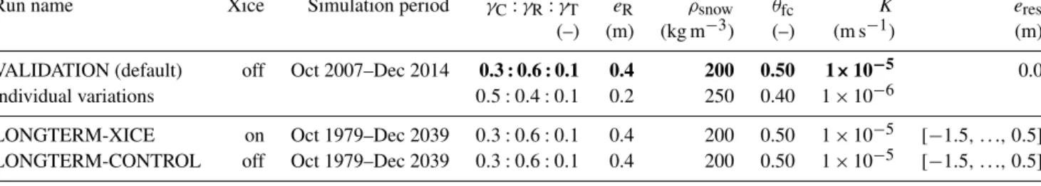
Table 4.Overview of the configurations used for validation and long-term model runs. Each of the default parameters shown in bold has been varied during the validation runs to the value specified in the line below while the remaining parameters were kept at their default values.

Run name Xice Simulation period γ_C:γR:γT eR ρsnow θ_fc K eres

(–) (m) (kg m⁻³) (–) (m s⁻¹) (m)

VALIDATION (default) off Oct 2007–Dec 2014 0.3 : 0.6 : 0.1 0.4 200 0.50 1×10⁻⁵ 0.0

individual variations 0.5:0.4:0.1 0.2 250 0.40 1×10⁻⁶

LONGTERM-XICE on Oct 1979–Dec 2039 0.3:0.6:0.1 0.4 200 0.50 1×10⁻⁵ [−1.5, . . .,0.5] LONGTERM-CONTROL off Oct 1979–Dec 2039 0.3:0.6:0.1 0.4 200 0.50 1×10⁻⁵ [−1.5, . . .,0.5]

compared to the measured values. For 2013 all model runs significantly underestimated the maximum ALT of the centres (by about 0.3 m) compared to the measured values. This can probably be attributed to too little precipitation in the forcing data, leading to an overly dry, and hence insulating, upper organic soil layer. The ALTs of the simulations with an increased areal fraction of the centres (γC=0.50) and with lower-elevated rims (eR=0.20 m) were particularly shallow during the final 3 years of the validation period, highlight- ing the sensitivity of the thermal regime to microtopographic characteristics.

The modelled ALT progressions for polygon rims were within the range of available measurements during all years of the validation period, resulting in good agreement with re- spect to both the timing of thawing and the maximum ALT.

The underestimation of ALT for the centres that occurred in 2013 was not observed for the rims. There was generally a very low variability among the validation runs, indicating that the modelled ALTs for the rims were less susceptible to changes in the varied parameters (γC/R/T,eR,ρsnow,θfc,K) than those simulated for the centres. This can probably be attributed to larger differences among the hydrological regimes of the centres among the different validation runs.

In addition to the ALT, we also compared modelled and measured soil temperatures within the active layer, for both polygon centres and polygon rims (see Fig. E1 in Ap- pendix E). A detailed assessment of the model performance in terms of root-mean-squared error (RMSE), bias, and coef- ficient of determination (R²) is provided in Tables F1 and F2 in Appendix F. For the default parameters, there was a slight cold bias (≥ −0.4^◦C) for the simulated rim temperatures while the centre temperatures showed a slight warm bias (≤0.52^◦C).R²values were in the range of 0.69 to 0.83 for the centres and between 0.79 and 0.90 for the rims, indicating an overall good reproduction of the temperature evolutions.

3.2.2 Ground hydrological regime

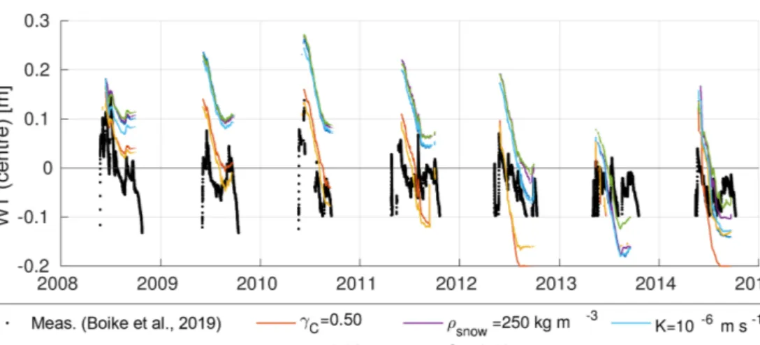
The hydrology scheme incorporated into CryoGrid 3 (see Sect. 2.2.3) made it possible to simulate a dynamic water table; we compared the modelling results with in situ WT measurements from a polygon on Samoylov Island (see Fig. 1 for the location of the measurement polygon). Figure 6 shows

the modelled and measured WT evolution in the polygon centre during the summer months of the validation period.

With the exception of 2013, the simulated WT evolutions showed a large range of about 0.1 to 0.2 m among the most extreme runs. For some years (e.g. 2011) there were runs in which the centres were water-covered throughout the entire summer while for the runs withγC=0.50 andeR=0.20 m WT was mostly below the soil surface. This suggests that the simulated WT of the centres is very sensitive to the topology and microtopography of the polygonal tundra and feeds back on the simulated ALT as mentioned above. Note that for these runs the RMSE was smaller for the simulated WTs but larger for the simulated ALT of the centres (Table F1) compared to the remaining runs, indicating the complex in- terplay among microtopography, hydrology, and the active layer. There was a general pattern in the simulated WT evolutions that was independent of the year and the parameter setting used: WTs were high immediately after snowmelt, usually followed by a decrease over the summer months after which the WTs stabilized towards the end of summer or increased again in response to major precipitation events.

The measured WTs lay mostly within the range of the simulated WTs. During most summers the measured WTs were partly above and partly below the soil surface. In most years the measured WT evolutions revealed a similar pattern to the modelled evolutions, with high WTs after snowmelt followed by a decrease towards the end of the summer. However, the measurements showed a more pronounced intra-annual variability than the individual model runs. In contrast, the inter- annual variability appeared to be slightly greater in the model runs. The remaining mismatches between modelling results and measurements were attributed to a variety of factors including (i) site-specific characteristics of the measurement polygon, (ii) the accuracy of the precipitation forcing data used in the model, (iii) the accuracy of measured WT values, and (iv) the simplistic representation of vertical and lateral water fluxes in the model.

Apart from WT we also compared modelled and measured soil moisture levels within the active layer, for both polygon centres and polygon rims (see Fig. E2 in Appendix E). There was a good agreement between modelled and measured soil moisture levels for the mostly water-saturated centre, while

(11)

Figure 5.Modelled and measured progression of the active layer thicknesses (ALTs) of polygon centres(a)and rims(b)for the 7-year period of the validation runs. The black markers represent the means and standard deviations of categorized CALM data (n=39 measurement points for centres,n=80 for rims) described in Boike et al. (2019). Coloured lines correspond to the individually modelled ALTs of the six validation runs (see Table 4 VALIDATION for default parameter values.). Note that the ALTs refer to unfrozen soil, excluding water bodies, so that positive values of ALT may occur if a water body is present.

Figure 6.Modelled versus measured water tables (WTs) relative to the soil surface of a polygon centre for the 7-year period of the validation runs. The measured data are for a particular polygon centre on Samoylov Island described by Boike et al. (2019). Coloured lines correspond to the individually modelled WTs of the six validation runs (see Table 4 VALIDATION for default parameter values). Note that minimum WT measurements are limited to a level of−0.120 m until 2009 and to−0.095 m from 2010.

(12)

the model underestimated soil moisture by about 10 % close to the surface of the rim profile. The latter can be attributed to uncertainty in the parameters (e.g. θfc, Table 2) and the assumption of instantaneous infiltration.

The model performance in terms of RMSE, bias, andR² for the simulated ground hydrological regime, is presented in Tables F1 and F3 in Appendix F. The simulated WT had a positive bias (0.06 m) for the default parameters, while it was slightly negative-biased for the runs withγ_C=0.50 and e_R=0.20 m. Simulated soil moisture values showed mostly low dry-biases (≥ −0.08) and fairR² values ranging from 0.39 to 0.76 for the centres and from 0.57 to 0.74 for the rims.

3.2.3 Summer surface energy balance

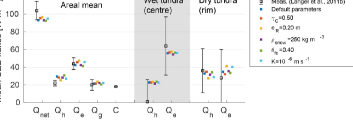
We used eddy-covariance measurements from Samoylov Is- land obtained between 7 June and 30 August 2008 (Langer et al., 2011b) to assess the model’s ability to reproduce the spatial heterogeneity in the SEB of polygonal tundra. We first compared measured mean surface energy fluxes⁴(net radia- tionQ_net, sensible heat fluxQ_h, latent heat fluxQ_e, ground heat fluxQg) with the modelled area-weighted mean fluxes for the same period in the validation runs (Fig. 7, left-hand side). The variability in all SEB components among the different model runs was low and they were all close to, or within, the uncertainty range of the measured fluxes. The measured summer Bowen ratio was 0.50, which compares reasonably well with the mean modelled value of 0.64. Note that the low variability in the modelled SEB partitioning indicates that it is robust against variations in the topology and microtopography of the polygonal tundra, as well as snow properties and hydrological parameters.

We next compared the turbulent heat fluxes (Q_h,Q_e) of wet tundra estimated from field measurements with those modelled for the centre tile (Fig. 7, central part). While the modelled fluxes lay within the large uncertainty range of the fluxes measured in the field, the mean modelled summer Bowen ratio of 0.40 was larger than the measured value of 0.02. However, the SEB partitioning for the centre tile in the model was significantly distinct from the area-weighted mean SEB.

Similarly, the modelled turbulent heat fluxes for the rim tile were of comparable magnitude to the fluxes for dry tundra estimated from field measurements (Fig. 7, right-hand side). The mean summer Bowen ratio for the rims in the model runs was 0.89, while the measured value was 1.29.

Like for the wet tundra described above, the model was able to reproduce a SEB partitioning for the rim tile that was distinct from the area-weighted mean SEB.

Although the spatial heterogeneity was more pronounced in the measured data than in the modelling results, the model

4The eddy-covariance measurement footprint was about 200 m in diameter.

was able to reproduce spatially heterogeneous patterns of turbulent heat fluxes while also robustly reflecting the mean summer SEB partitioning of the polygonal tundra.

3.2.4 Snow redistribution

To assess the ability of the snow redistribution scheme to reproduce actual, spatially heterogeneous SD distributions, we compared modelled and measured SDs for spring 2008 in polygon centres and rims as well as the areal mean SD (Fig. 8). The modelled areal mean SDs of the validation runs were close (≤0.07 m) to the measured value of 0.31 m. Mod- elled areal mean SDs were slightly higher for those runs with lower snow density (ρ_snow=200 kg m⁻³) and agreed very well with the measured value for the run withρsnow= 250 kg m⁻³. The modelled SDs for polygon centres were consistently higher (mean of all runs: 0.60 m) than the measurements which had a mean of about 0.46 m. Similarly, the modelled SDs of the rims were on average (mean of all runs:

0.23 m) higher than the measurements (mean: 0.18 m), but were overall closer to the field data than those for the centres.

The parameter variations further revealed that while the areal mean SDs are only sensitive to snow density, the spatial distribution of SDs is critically influenced by variations in the topology (γ_C/R/T) and microtopography (e_R) of polygonal tundra. The comparison showed that the model was able to realistically reproduce the spatial heterogeneity in SD. Fur- thermore, the variability within the validation runs was similar to that found in the measurement data collected from an area that contained several polygons.

3.3 Summary

The comparison of modelled and measured ALT, WT, SEB, and SD (plus soil temperature and soil moisture in Ap- pendix E) justified the use of a tile-based modelling approach as the measured spatial heterogeneities in (i) the subsurface thermal and hydrological regimes, (ii) the surface energy balance, and (iii) the snow distribution of polygonal tundra were well reproduced in the model validation runs. The sensitivity tests revealed that the simulated ALT and WT evolutions are robust against variations in snow and hydrological parameters (ρ_snow,θ_fc,K), while the polygon microtopography (γ_C, e_R) had a significant impact on simulated SD, WT, and ALT.

4 Results

4.1 Ice-wedge degradation under intermediate hydrological conditions (e_res=0.0 m)

The primary objective of our study was to simulate the transient process of ice-wedge degradation in a tile-based model of polygonal tundra. For this we conducted 60-year runs of our model setup with the excess ice module being enabled (see Table 4, LONGTERM-XICE). The run with an interme-

(13)

Figure 7.Modelled and measured partitioning of the mean surface energy balance (SEB) during summer 2008 (7 June–30 August). Modelled values are displayed in individual colours for each of the six validation runs (see Table 4 VALIDATION for default parameter values). The measured data are mean summer fluxes from Langer et al. (2011b) and the error bars indicate the estimated accuracies provided in that publication. The left-hand side (white background) shows the overall SEB (area-weighted mean of all tiles for the model), the central part of the figure (grey background) shows turbulent fluxes for wet tundra (centre tile for the model), and the right-hand side (white background) shows turbulent fluxes for dry tundra (rim tile for the model).

Figure 8.Modelled and measured snow depths (SDs) for polygon centres and polygon rims, together with the areal mean. The data from Boike et al. (2013) show the mean and standard deviation of spatially distributed point measurements obtained between 25 April and 2 May 2008. Modelled values correspond to SDs on 1 May 2008 and are displayed in individual colours for each of the six validation runs (see Table 4 VALIDATION for default parameter values).

diate water level in the external water reservoir (e_res) of 0.0 m illustrated the degradation process and the associated microtopographic changes very well (Fig. 9). The Supplement to this article contains an animated video showing the results of this simulation run.

LCP phase.During the first decade of the simulation period (1980–1990) the modelled polygonal tundra was low- centred (LCP, according to Eq. 1 above). During this period the centre tile was (over-)saturated with water, resulting in surface water of 0.05 to 0.2 m in depth. The rims were rather dry with end-of-summer WTs about 0.2–0.3 m below the surface. The absolute altitude of the modelled end- of-summer WT was almost identical for the centre (1986:

WT_C=20.20 m) and rim tile (1986: WT_R=20.15 m), indicating lateral water fluxes that lead to a levelling out of the WT within the active layer between the different tiles. Dur- ing the LCP phase the troughs showed a very shallow ALT of about 0.2 m in depth and their active layer was mostly dry

with water tables either absent or just above the frost table.

Note that during the first 9 years of the simulation period the active layer of the trough tile did not extend below the water level in the external water reservoir (20.0 m a.s.l.), so that any water in the troughs drained into the external reservoir.

Transition.During the last 5 years of the LCP phase (1986 to 1990) the troughs started to subside as soon as the active layer extended into the intermediate excess ice layer, which lay between 0.2 and 0.5 m in depth and contained 20 % excess ice (see Table 3). Concurrent with the subsidence of the ground surface the end-of-summer ALT almost doubled from 0.20 m in 1986 to 0.38 m in 1991. During these years the water saturation in the active layer beneath the troughs increased (with the WT lying above ALT) due to the addition of water from the melting of excess ice and lateral fluxes from the rims, which occur every summer as soon as the frost table of the troughs sinks below the water table of the rims. The increased amount of liquid water in the active layer beneath

(14)

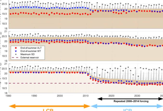
Figure 9.Evolution of the polygonal tundra tiles for the 60-year run (from 1980 to 2040) withe_res=0.0 m (see Table 4, LONGTERM- XICE). Each panel displays the temporal evolution of the vertical extents of snow cover, water body, and soil domains (excess ice and no excess ice) for the different tiles (a: centre;b: rim;c: trough). For the excess ice layers, lighter colours indicate larger amounts of excess ice. The end-of-summer (maximum) active layer depth (ALT), the end-of-summer water table (WT), and the maximum snow depth (SD) are also indicated for each year. The initial low-centred polygon (LCP) phase lasted for about 11 years, followed by a transitional phase of ice-wedge degradation and ground subsidence (ICP) until the start of the high-centred polygon (HCP) phase. Note that the meteorological forcing after 2014 consisted of repeated appending of the forcing between 2000 and 2014. A condensed plot of the results is shown in Fig. 10.

The Supplement to this article contains an animated video showing the results of this simulation run.

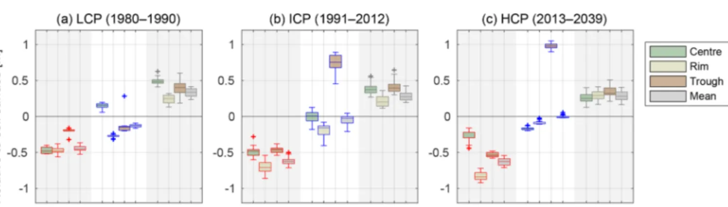
Figure 10.Box plots of the distributions of maximum ALT, WT, and SD for each tile and the area-weighted means from all years of the respective phases of the polygonal tundra, from the LCP phase(a), through the ICP phase(b), to the HCP phase(c). The transition from LCP to HCP implies shifts in the thermal and hydrological regimes of the different landscape tiles; it also affects the snow distribution. The results are for the long-term run witheres=0.0 m, which is also shown in Fig. 9.

(15)

the troughs increased its thermal conductivity, resulting in increased ground heat flux (with the mean summer Qgin the trough tile increasing from about 8 W m⁻²in 1986 to about 36 W m⁻² in 1991) which in turn resulted in a further increase in the ALT. This positive feedback led to continued melting of excess ice and subsequent ground subsidence in the following years. In the year 1989 of the simulation the thaw front extended into the ice-rich layer representing the ice-wedge which contained 35 % of excess ice (see Table 3).

The increased amount of melted excess ice pooled up in the active layer and enhanced the positive feedback described above.

ICP.During the summer of 1990 of the simulation the soil altitude of the troughs subsided below that of the centre tile, such that the polygons represented by the tiles were clas- sified as ICPs, according to Eq. (2) above. After the first 2 years of the ICP phase (1990–1991), during which the troughs subsided very rapidly (about 0.2–0.3 m a⁻¹), the subsidence rate decreased to about 0.05–0.1 m a⁻¹in subsequent years, with a number of summers recording no ground subsidence at all. The total subsidence of the troughs between 1990 and 2012 amounted to about 1.0 m. The depth of the water body ponded in the troughs was about 1.0 m in 2012.

During the ICP phase the rims also started to subside as soon as the active layer extended into the excess ice layer for the first time (extending downwards from 0.6 m in depth with 20 % excess ice; see Table 3). The subsidence continued for about 2 decades but at a lower rate than the troughs, which had a higher excess ice content. During the simulation period from 1990 to 2012 the polygon rims subsided by a total of 0.4 m, reaching the level of the centre tile, so that the modelled polygonal tundra was subsequently centred high (HCP, according to Eq. 3 above). Note that during the ICP phase the active layer of the polygon rims became wetter as the absolute altitude of the WT remained more or less constant while the soil surface subsided. The polygon centres remained mostly water-saturated during the ICP phase, with their WT sinking below the soil surface in only a few of the summers.

HCP.The HCP phase lasted from 2012 until the end of the simulation period in 2040. The subsidence rates for both rim and trough tiles were significantly lower than during the ICP phase. No ground subsidence occurred in any of the tiles during the last decade of the simulation. The water levels in all tiles also stabilized and showed less inter-annual variability.

As soon as the centres became the highest part of the landscape their WT dropped to about 0.2 m below the surface.

The resulting organic-rich dry upper layer had an insulating effect so that the maximum ALT of the centre tile was sub- stantially lower during the HCP phase than during the pre- ceding LCP and ICP phases.

All of the stages of polygonal tundra evolution defined in Sect. 2.2.1 occurred during the 60-year simulation period of the run with an intermediate water level in the external water reservoir (e_res=0.0 m): the LCP phase lasted for 10 years,

from the start of the simulation in 1980 until the summer of 1990, followed by the ICP phase that lasted for 22 years (until summer 2012) and the HCP phase that continued for the remaining 27 years. The key characteristics of the different phases are summarized in Fig. 10, which shows box plots of the distributions of end-of-summer ALT, end-of-summer WT, and maximum SD for each tile, together with the area- weighted means for the entire landscape. The transition from LCP to HCP led to an increase in the maximum ALT for polygon rims and troughs but a reduced maximum ALT for the polygon centres. These changes were directly linked to the changes in WTs, which fell from above the surface of the centres during the LCP phase to below the surface during the HCP phase. For the polygon rims and troughs the WT increased such that the landscape-mean WT elevation relative to the soil surface increased slightly, indicating that the polygonal tundra was becoming wetter. The snow distribution, which was heterogeneous during the LCP phase with a high SD for centres and troughs, becomes increasingly ho- mogeneous during the HCP phase in which the surface altitudes of the three tiles were similar.

In summary, the run with intermediate hydrological conditions (e_res=0.0 m) demonstrated that the tile-based approach to modelling a polygonal tundra landscape is able to simulate the degradation of ice wedges and the associated geomorphological transition from low-centred polygons to high-centred polygons.

4.2 Variation in the hydrological conditions

The second objective of our study was to investigate the control that hydrological conditions exert on the evolution of polygonal tundra. For this we considered the results of addi- tional long-term runs with different water levels in the external water reservoir (e_res; see Table 4, LONGTERM-XICE).

To contrast the results for the run withe_res=0.0 m discussed in Sect. 4.1, we analysed in detail another model run with a rather low value fore_resof−1.0 m, corresponding to draining hydrological conditions (Sect. 4.2.1). We also compared the evolution of the polygonal tundra in all runs with the excess ice scheme enabled, covering a broad range of hydrological conditions (Sect. 4.2.2).

4.2.1 Draining hydrological conditions (e_res= −1.0 m) The temporal evolution of the tiles is shown in Fig. 11 and the characteristics of the different phases are summarized in Fig. 12. The Supplement to this article contains an animated video showing the results of this simulation run.

LCP.The landscape evolution for this setting can be di- vided into two phases. During the first 3 decades of the simulation period (1980–2010) the polygonal tundra remained centred low, with the polygon centres being water-covered, the rims were stable (i.e. not subsiding) with an end-of- summer WT about 0.3 m below the surface, and the troughs

(16)

Figure 11.Evolution of the polygonal tundra tiles for the 60-year run (from 1980 to 2040) and well-drained hydrological conditions (e_res=

−1.0 m). Ice-wedge degradation started about 2 decades later than in the run with a water level in the external reservoir (eres=0.0 m – Fig. 9), ultimately leading to an overall lowering of the water tables and effective drainage of the landscape. Note that the meteorological forcing after 2014 consisted of repeated appending of the forcing between 2000 and 2014. A condensed plot of the results is shown in Fig. 12.

The Supplement to this article contains an animated video showing the results of this simulation run.

Figure 12.Box plots of the distributions of maximum ALT, WT, and SD for each tile and the area-weighted means from all years of the respective phases of polygonal tundra, from the LCP phase(a)to the ICP phase(b). Note that the HCP phase is not attained during this run.

The results are for the long-term run withe_res= −1.0 m, which is also shown in Fig. 11.