Blood Distribution and Energy Metabolism of the Brain of Polar cod (Boreogadus saida) Under Ocean Acidification
Erasmus Mundus International M.Sc. in Marine Biological Resources (IMBRSea)
Applied Ecology and Conservation
Alfred-Wegener-Institute, Helmholtz-Centre for Polar and Marine Research Division Biosciences
Section Integrative Ecophysiology
Thesis candidate: Jan Phillipp Geißel, B.Sc.
Reference number: 20170579
janphillipp.geissel@imbrsea.eu Thesis supervisor: Dr. Christian Bock
presented the 05th of August 2019
Declaration of authorship
I hereby declare that the thesis submitted is my own work. All direct or indirect sources used are acknowledged as references.
Data ownership
No data can be taken out of this work without prior approval of the thesis supervisor and the author.
I Table of contents
I. Abbreviations and symbols ... III II. Figures ... IV III. Tables ... I
1 Executive summary ... 1
2 Abstract ... 1
3 Introduction & Aims ... 1
3.1 Ocean Warming and Acidification (OWA) and Ecological Consequences ... 1
3.2 Model species... 3
3.3 Cellular energy metabolism, acid-base regulation, intracellular pH ... 3
3.4 Blood distribution ... 4
3.5 Magnetic Resonance Imaging (MRI) ... 6
3.6 31P-NMR Spectroscopy ... 7
3.7 Aims ... 10
4 Materials & Methods ... 11
4.1 Specimens and animal maintenance ... 11
4.2 Water supply and seawater chemistry ... 12
4.3 Experimental setup and protocol ... 13
4.4 Nuclear magnetic resonance imaging and spectroscopy ... 15
4.4.1 Experimental protocol ... 15
4.4.2 MR imaging and spectroscopy protocol ... 16
4.4.3 Image Analysis ... 17
4.4.4 Statistical analysis ... 20
5 Results ... 21
5.1 Brain morphology ... 21
5.2 Blood Flow and Perfusion ... 23
5.2.1 Vascular morphology ... 23
II
5.2.2 Angiography scans ... 23
5.3 In vivo measurement of blood distribution of the brain of polar cod ... 26
5.3.1 Method Application ... 26
5.4 In vivo measurement of intracellular pH and the energy metabolism of the brain of polar cod ... 40
5.4.1 Indices for the cellular energetic state in vivo. ... 40
5.4.2 In vivo measurement of intracellular pH and the energy metabolism of the brain of polar cod 44 6 Discussion ... 48
6.1 Method Development and Evaluation ... 48
6.2 Effects of Ocean Acidification ... 50
7 Conclusion ... 56
8 Acknowledgements ... 57
9 References ... 58
10 Annex ... 64
10.1 Phantom trials ... 64
10.1.1 Titration curve ... 65
III I. Abbreviations and symbols
ASL arterial spin labelling ATP adenosine tri-phosphate
B0 magnetic field, represents net magnetization vector in MRI BOLD blood oxygenation level dependent
CASL continuous ASL
CBF cerebral blood flow CBV cerebral blood volume
cm centimetre
FAIR flow-sensitive alternating inversion recovery FLASH fast low angle shot
FID free induction decay fMRI functional MRI
IPCC Intergovernmental Panel on Climate Change MIP maximum intensity projection
MR magnetic resonance
MRI magnetic resonance imaging MTT mean transit time
NMR nuclear magnetic resonance OA ocean acidification
OW ocean warming
OWA ocean warming and acidification
PASL pulsed ASL
pCO2 partial pressure carbon dioxide PCA phase contrast angiography
PCr phosphocreatine
pHe extracellular pH pHi intracellular pH Pi inorganic phosphate
pK logarithmic acid dissociation constant PWI perfusion weighted imaging
RARE rapid acquisition with relaxation enhancement rCBF regional cerebral blood flow
RCP representative concentration pathway ROI region of interest
SNR signal-to-noise-ratio SST sea surface temperature
T Tesla, derived unit of magnetic induction T1 longitudinal relaxation time
T1A apparent T1
T2 transversal relaxation time T2* spin-spin-relaxation time TA acquisition time
TE echo time
ToF time of flight angiography TR repetition time
µm micrometre
δ chemical shift
ν frequency
µatm micro atmosphere
IV II. Figures
Figure 3-1 In vivo 31P-NMR spectrum calibrated to PCr as 0 ppm illustrating the
measurement of the chemical shift (δ) of Pi in relation to PCr. ... 9
Figure 4-1 Photo of a polar cod (Boreogadus saida) in its habitat (photo: Hauke Flores/AWI). ... 11
Figure 4-2 Technical drawing of the experimental setup. ... 12
Figure 4-3 Technical drawing of the in-house built experimental chamber. ... 14
Figure 4-4 Experimental chamber at the positioning device in front of the MRI. ... 14
Figure 4-5 Photo of the used MRI and positioning device. ... 15
Figure 4-6 Example of an axial FLASH scan in vivo with marked ROIs for the evaluation of blood flow. ... 18
Figure 5-1 Comparison of two different MR imaging techniques. ... 22
Figure 5-2 Morphological RARE MRI scans of the brain of polar cod. ... 22
Figure 5-3 Example axial FLASH scan of a Polar cod head. ... 23
Figure 5-4 3D Angiography MIP axial plane in anterior view. ... 24
Figure 5-5 3D Angiography MIP in the coronal plane dorsal view. ... 25
Figure 5-6 3D Angiography MIP sagittal plane. ... 25
Figure 5-7 example axial phase contrast imaging scans. ... 26
Figure 5-8 Axial phase contrast imaging scan of fish 6 with ROIs annotated in their respective position. ... 27
Figure 5-9 Time series of measured blood flow in ROI 1, ROI 2 and ROI 3 in fish 6. 28 Figure 5-10 Time series of measured blood flow in ROI 1, ROI 2 and ROI 3 in fish 7. ... 30
Figure 5-11 Time series of measured blood flow from phase contrast imaging in ROI 4, ROI 5 and ROI 6 in fish 7. ... 31
Figure 5-12 FLASH axial MRI image annotated with ROIs of Polar cod (fish 6) in vivo ... 32
V Figure 5-13 Time series of signal intensity from T1-weigthed imaging in ROI 1-4 in fish 6. ... 33 Figure 5-14 Time series of measured signal from T1-weigthed imaging intensity in ROI 1-4 in fish 7. ... 34 Figure 5-15 BOLD axial MRI image annotated with ROIs of Polar cod (fish 6) in vivo.
... 35 Figure 5-16 Time series - BOLD in vivo MRI scans of fish 6 in ROI 1- 4 in fish 7. .... 37 Figure 5-17 BOLD axial MRI image annotated with ROIs of Polar cod (fish 7) in vivo.
... 38 Figure 5-18 Time series - BOLD in vivo MRI scans of fish 7 in ROI 1-3 in fish 7. ... 39 Figure 5-19 Boxplots showing the Pi-PCr-ratio for fish 6 and fish 7 compared by experimental category (post handling, control, treatment, post treatment). ... 40 Figure 5-20 Boxplots showing the βATP signal intensity for Fish 6 and Fish 7 compared by category (post handling, control, treatment, post treatment). ... 41 Figure 5-21 Time series plots of the Pi-PCr-ratio (top) and βATP signal intensity in fish 6 over time. ... 42 Figure 5-22 Time series plots of the PI/PCr-ratio (top) and βATP concentration in fish 7 time. ... 43 Figure 5-23 Comparison of sum spectra of a fish after handling and after 18h post handling. ... 44 Figure 5-24 Time series of pHi from 31P NMR over the post-handling acclimation phase. ... 45 Figure 5-25 31P NMR sum spectrum showing a double peak around the δ of Pi. ... 45 Figure 5-26 Boxplots showing the intracellular pH (pHi), calculated from chemical shift, for fish 6 and fish 7 compared by experimental category (post handling, control, treatment, post treatment). ... 46 Figure 5-27 Time series of the pHi by condition. ... 47 Figure 10-1 Photo of a phantom solution injected into a sealed glass vial. The vial was positioned within an experimental chamber. ... 66
VI Figure 10-2 Titration curve. ... 68
I III. Tables
Table 1 Seawater alkalinity parameters ... 12 Table 2 measured chemical shifts of the 31P-NMR spectroscopy phantom trials. .... 64 Table 3 chemical composition of the 31P-NMR Spectroscopy phantoms ... 66
1 Executive summary
Polar cod (Boreogadus saida) is a key species of the arctic food web. It has a linking function between the trophic level of zooplankton and the top predators like marine mammals and seabirds. Under climate change and it shifts its distribution northwards and decreases in numbers. Under ocean acidification, by increased CO2 accumulation, polar cod exhibits alterations in its neurochemical profile as well as behavioural alterations. The underlying factors are still poorly understood. In airbreathing vertebrates, increased concentrations of CO2 (hypercapnia) leads to increased cerebral blood flow, so it was suggested that one of the underlying factors of those behavioural alterations might be accompanied by increased cerebral blood flow.
Besides potential changes in the blood distribution, elevated environmental CO2 might affect the acid-base status of the brain and its energy metabolism. Therefore, this study aimed to adapt an array of non-invasive magnetic resonance imaging (MRI) techniques to investigate potential changes in the blood distribution of the brain of polar cod under ocean acidification accompanied with measurements of the intracellular pH and energy status of the brain cells. To investigate blood flow, phase contrast MR imaging, FLASH MR imaging and BOLD imaging were adapted and successfully used under control conditions and conditions of elevated CO2 concentrations in seawater. These investigations were complimented by in vivo 31P-NMR spectroscopy to investigate potential changes in intracellular pH and energy metabolism. The presented study attained to deliver the first multi-parametric datasets, investigating blood supply on different levels of the vascular system of the head combined with observations of the acid-base and energy status of the brain of polar cod. Fluctuations in blood flow and perfusion were observed, but no significant elevation could be identified under ocean acidification. Ocean acidification induced decreases in intracellular pH were subtle and compensated for completely within 24 hours. No substantial alterations in the energy metabolism of the brain were detected under elevated CO2. This study confirms previous work that found that the regulation of the acid-base status in the fish brain was fast and complete and advanced the current knowledge about the effects of ocean acidification on cerebral blood flow in fish. While previous works found showed that venous and arterial blood flow velocities in polar cod were decreasing under CO2 this study did not find suspected CO2 dependent blood flow alterations in the vasculature of the head.
2 Abstract
Polar cod (Boreogadus saida) is a key species of the arctic food web and links trophic levels. Under ocean acidification (OA), the accumulation of CO2, polar cod exhibits neurochemical alterations as well as behavioural alterations. The underlying factors are still poorly understood. In airbreathing vertebrates, increased CO2 concentrations (hypercapnia) cause increased cerebral blood flow (CBF). Besides potential changes in the blood distribution, elevated environmental CO2 might affect the acid-base status of the brain and its energy metabolism. Therefore, this study aimed to adapt an array of in vivo magnetic resonance imaging (MRI) techniques to investigate potential changes in the blood distribution of the brain of polar cod under OA. To investigate blood flow, phase contrast MRI, FLASH MRI and BOLD imaging were adapted and used under control conditions and conditions of elevated CO2 concentrations. These investigations were complimented by in vivo 31P-NMR spectroscopy to investigate potential changes in intracellular pH and energy metabolism. Fluctuations in blood flow and perfusion were observed but no significant elevations could be identified under OA. OA induced decreases in intracellular pH were subtle and compensated for completely within 24 hours. No substantial alterations in the energy metabolism of the brain were detected under elevated CO2.
3 Introduction & Aims
3.1 Ocean Warming and Acidification (OWA) and Ecological Consequences The extensive burning of fossil fuels and the resulting emission of CO2 and other greenhouse gases to the atmosphere have already caused warming of the earth, including the oceans. This warming will continue over the 21st century even though there are different predictions about its extent. This ocean warming will lead to rising sea levels due to thermal expansion and melting ice, decreased sea-ice extend and altered ocean circulations (IPCC 2013). The rising temperature poses threats to a broad variety of marine organisms and biota associated with the sea on all trophic levels. (Alexander et al. 2018). Not only form those organisms an integral part of the marine ecosystem and provide important, ecosystem services but also provide an essential part of the food security of many countries and societies. Fish for example accounted for 16.6 percent of the world’s intake in animal protein in 2009 (FAO 2012).
Especially in the Arctic Ocean physical and biological conditions are changing at unprecedented rates (Gaston et al. 2003, Polyakov et al. 2005). Physical factors such as an elevated SST and decreased sea ice coverage lead to serious shifts in the biogeography of fish stocks, their temporal and spatial distribution and abundance.
(Gaston et al. 2003, Pörtner & Knust 2007, Pörtner et al. 2008) Additionally, to global warming, the oceans pH decreases by carbon dioxide (CO2) intake from the atmosphere to the water. This process is known as ocean acidification (OA). CO2
dissolves in the ocean and reacts with seawater in a process that forms carbonic acid.
Hereby the ocean acidifies the partitioning of inorganic carbon shifts towards increased CO2 and dissolved inorganic carbon and decreased carbonate ions concentrations.
Ocean surface pH has already decreased by 0.1 units compared to pre-industrial times (Field et al. 2014). The further decrease in pH depends on both the future emissions of carbon dioxide and the emissions pathways (Representative Concentration Pathways (RCP)) as projected by the Intergovernmental Panel on Climate Change (IPCC) for the end of the century (IPCC 2013). Under unabated emissions ocean surface pH might decrease about 0.4 units compared to pre-industrial times by the end of the 21st century (Field et al. 2014, Gattuso et al. 2015). In the Arctic these alterations in pH and pCO2 may even be stronger and faster due to the high solubility of gases in cold water (Fransson et al. 2009). The Representative Concentration Pathway (RCP) projects a sea surface temperature (SST) rise of 4 to 11 °C for the Arctic in the business-as-usual case (RCP 8.5, IPCC 2014) accompanied by a partial pressure of
Introduction & Aims
2 carbon dioxide (pCO2) rise from 400 µatm to 1370 µatm. High CO2 levels affect marine biota on all trophic levels and has acute impacts on vital physiological functions and chronic impacts on vital aspects of their life cycles (Ishimatsu et al. 2005, Esbaugh 2018). Under high ambient pCO2, CO2 diffuses into animals via their epithelia decreasing first the extracellular pH (pHe) and then in intracellular compartments. In tissue, the formation of carbonic acid is catalysed through carbonic anhydrase under hypercapnia. This facilitates a balance of acid-base equivalents, namely H+ and HCO3-
(Clairborne et al. 2002).
The effects of elevated CO2 concentrations in sea water are diverse. Albeit a present lack of knowledge about the extent of the ecological consequences of high CO2
concentrations in the world’s oceans variety of effects were demonstrated. Elevated CO2 concentrations will affect fish due acute, potentially lethal, effects on vital physiological functions as well as due to chronic, sublethal impacts on other aspects of their life cycle. Lethal pCO2 appears to vary between species and especially early life stages are sensitive to high CO2 (Ishimatsu et al. 2005)
Especially behavioural changes in a high CO2 world are of interest as studiesshowed that certain species exhibit altered behaviour under simulated ocean acidification (Ishimatsu et al. 2005, Tresguerres & Hamilton 2017). Polar cod (Boreogadus saida) for example exhibits behavioural disturbances like significantly reduced absolute laterality and a shift in relative laterality under elevated CO2 (Schmidt et al. 2017a).
Also, neurochemical alterations in the brain of polar cod like an significant increase in GABA at high pCO2 (Schmidt et al. 2017b). In Atlantic cod (Gadus morhua) studies could show strong aversive behaviour towards water with increased pCO2 (Jutfelt &
Hedgärde 2013). In vivo magnetic resonance imaging (MRI) and spectroscopy (NMR) studies revealed, that the acid base regulation in the brain is particularly affected under elevated CO2 concentrations (Wermter et al. 2018). Active acid base regulation of the brain is an energy consuming process and appears to be limited in polar cod under OWA (Schmidt et al. 2017b).
Introduction & Aims
3 3.2 Model species
In this study polar cod (Boreogadus saida) was used as model species. As being highly specialist to cold water and polar regions, polar cod is critically affected by ocean warming and acidification. Polar cod has its temperature range from -2 to +8°C. (Drost et al. 2014) and is regularly associated with sea ice. The are considered demersal or semi-pelagic with a strong surface orientation of eggs and larvae and an orientation to deeper habitats including demersal habitats at the end of their first year (Geoffroy et al. 2016). The distribution ranges of polar cod appear to have shifted northwards with decreasing numbers at the edges of their distribution and reduced numbers in years with reduced sea ice cover (Mueter et al. 2016). Recent studies predicted further habitat losses in polar cod under OA due to a narrowing of thermal ranges during the embryonic development (Dahlke et al. 2018) and behavioural alterations (Schmidt et al. 2017a). Kunz et al. (2018) demonstrated that polar cod possesses reduced maximum swimming capacity after long time acclimation to future OAW conditions (RCP 8.5 scenario, IPCC 2014) even though they could not find significant differences in standard metabolic rate. The linking function of polar cod among trophic levels in the Arctic food web is at stake if the standing stock shifts its distribution further northwards, which might result in cascading ecological consequences. To be able to project ecosystem impacts caused by climate change, the assessment of tolerance ranges and acclimation capacities of key species is crucial (Kunz et al. 2018). Its predicted that under the predicted OWA scenarios Polar cod will show shifts in populations abundances and los crucial parts of its spawning grounds (Dahlke et al. 2018).
However, the underlying physiological factors that cause behavioural alterations are not well understood and there appears to be a knowledge gap. Possible factors like brain perfusion, alterations in the brain’s energy metabolism need further investigation.
3.3 Cellular energy metabolism, acid-base regulation, intracellular pH
Energy provision and consumption in fish is generally dependent on the levels and variability of activity and environmental factors. Different pathways contribute to the functional capacities if cells, organs and the whole organism. Energy demanding processes like ventilation, cardiovascular performance and acid-base regulation need to be fuelled.
Introduction & Aims
4 In the cellular energy metabolism, adenosine tri-phosphate (ATP) is the most important nucleoside phosphate in the energy pathway. Biological functions from the generation of mechanical work to the powering of ion-transporters is fuelled by metabolic energy in form of ATP. As in most vertebrates, in fish, more than 95% of the ATP required in the cell metabolism under resting conditions is derived from the aerobic metabolism based in mitochondria, i.e. oxidative phosphorylation.
In fish, there are two main anaerobic pathways produce ATP in fish when there is high availability of energy. The more relevant here is PCr hydrolysis following the formula:
creatine + ATP → phosphocreatine + ADP + H+
Under conditions of rapidly increasing energy demand or when oxygen is limited this process is reversed using PCr as store of high-energy phosphates that are easily and timely assessable. PCr can donate phosphates to ADP forming ATP. PCr as energy store allows fast energy transfer to ATP at rates far higher than by aerobic or anaerobic metabolism. As it is the first energy source to be used under high energy demand such as burst swimming it is used under handling stress, anoxia and possibly hypercapnia (Borger et al. 1998). The signal intensity of inorganic phosphates (Pi) rises with increased energy demand. In teleosts, PCr levels are typically high in energy demanding tissues like skeletal muscle and nervous tissue and low in other organs.
This allows its use in 31P NMR spectroscopy studies of the energy metabolism of muscles and brain.
Fish must maintain homeostasis of their intra- and extracellular pH like other vertebrates but face constraint due to the aquatic environment they are living in (Clairborne et al. 2002). Under normal conditions pH is tightly controlled in organisms due to its critical role for the function of cellular processes such as the energy metabolism. While the measurement of blood pH (i.e. extracellular pH (pHe)) is relatively simple, the accurate measurement of intracellular pH (pHe) in vivo is more challenging.
3.4 Blood distribution
One of the permanent tasks of blood is to provide the gas exchange, i.e. O2- transportation from the respiratory organs (e.g. gills) to the tissues where it is needed
Introduction & Aims
5 and in turn the removal of CO2. This is the case for all animals except Tracheata. In the respiratory organs, i.e. lungs and gills, O2 is incorporated and then distributed in the body by energy consuming processes like the heartbeat. The heart pumps the blood through arteries and from there through their smaller branches, the arterioles, and finally trough the capillaries. Capillaries, small blood vessel from 5 to 10 µm in diameter, forming a fine mesh, the capillary bed, where the actual exchange of gas and nutrients between the blood and the tissues happens. After the capillaries, the blood is transported by venules and veins back to the heart. This is true for those animals having a closed circulation system including vertebrates (Soldatov 2006).
Cartilaginous and bony fish are the first groups of organisms whose capillary networks are close to those of terrestrial vertebrates. They differ though in in reactivity of vessels to vasoactive compounds and ecological factors and show a heterogeneity of vessels in the capillary bed and a permeability of capillary units to organic compounds different to other vertebrates (Söderström & Nilsson 2000).
In vivo cardiac responses to hypercapnia vary amongst fish species. Similarly, corresponding blood pressure responses vary amongst species. Bradycardia appears to be a common but not universal response to hypercapnia among teleosts (Perry &
Gilmour 2006). In rainbow trout (Oncorhynchus mykiss), direct vasodilatory effects of elevated pCO2 on the peripheral vasculature were found (Mckendry and Perry 2001).
Other studies showed increased blood pressure in different species due to peripheral vasoconstriction. There appears to be no obvious pattern across teleost species (see Perry & Gilmour 2006 for review). In Atlantic cod (Gadus morhua), reduced cardiac output could be shown under severe hypercapnia (Gesser & Poupa 1983). Also, the contractile force in the myocardium of G. morhua has been shown to decrease under high CO2 to an extend lower than of compared species (Gesser & Jørgensen 1982).
Schmidt (2019) showed significantly lowered arterial and venous blood flow both in polar cod under increased CO2 (1668 ± 250 μatm)) and normal blood flow was not restored within the observation period of four days.
Perfusion is defined as the passage of blood through an organ’s vascular network, e.g.
the microcirculation trough the capillary bed of the brain. Perfusion can be assessed non-invasively by MRI measurements of cerebral blood flow (CBF), cerebral blood volume (CBV) and mean transit time (MTT). In mammals and other air breathing vertebrates, e.g. turtles, hypercapnia causes cerebral vasodilation which leads to
Introduction & Aims
6 increased CBF (Bickler 1992, Buchanan & Phillis 1993, Duelli & Kuschinsky 1993).
Currently there is poor knowledge about the regulation of cerebral blood flow (CBF) in fish and other “lower” vertebrates.
3.5 Magnetic Resonance Imaging (MRI)
In vivo magnetic resonance imaging (MRI) allows to study physiologic processes non- invasively in a living organism. MRI bears the advantages to allow scans of soft tissue (other than other imaging modalities like x-ray) and allows the measurement of flowing liquids (e.g. diffusion and perfusion) in a living organism, both physiologic and pathologic. Furthermore, MRI allows the characterization and discrimination among tissues using their physical and biochemical properties (water, iron, fat, and extravascular blood and its breakdown products). It provides three-dimensional non- invasive quantitative methods of cerebral blood flow (CBF) quantification.
Specific parameters were introduced for an understanding and characterisation of MR imaging contrast. In particular, the T1 relaxation time, also known as spin-lattice relaxation time, describes the time net magnetisation vector of an excited particles spin recovers to its ground state according with B0. T1-weighted imaging is frequently applied for separation of tissues by differences in image contrast, which depends on the different T1 relaxation times of different tissues. T2-relaxation-time describes the spin-spin-relaxation time. This refers to the progressive dephasing of the spin of the nuclei after the end of a 90° pulse. The time this dephasing takes is tissue-dependent.
T2 is long in pure water and comparably faster in macromolecules and tissues. T2*- weighted imaging is a MRI sequence used to quantify effective T2*, which depends in addition to T2 on local changes in the magnetic field homogeneity caused by minor differences in the chemical environment. T2*-weighting is therefore used for functional imaging.
Introduction & Aims
7 T1-weighted MR imaging (FLASH)
T1-weighted is a method advised for stationary anatomical applications. T1-weighted imaging is usually achieved using a gradient echo method (e.g. fast low angle shot (FLASH) or spin-echo sequence (such as Relaxation Enhancement (RARE) MR imaging) with a short repetition time (TR) (Matthaei et al. 1985). T1-weighted imaging methods exhibit a high signal intensity for fat, fatty bone marrow, paramagnetic contrast agents and slow flowing blood. The sensitivity for slow flowing blood makes it a method of particular interest for this study. FLASH methods allow the acquisition of time courses.
Blood oxygenation level dependent (BOLD) MR imaging
Blood oxygenation level dependent (BOLD) imaging is a T2*-weighted gradient echo method to generate images to assess differences in the ratio of oxygenated and deoxygenated blood (Ogawa et al. 1990). Oxygenated haemoglobin is diamagnetic and deoxygenated haemoglobin is paramagnetic. Paramagnetic materials induce changes in T2* values of tissues, therefore changes in oxygenated and deoxygenated ratio of blood can be followed up with this technique and is frequently used in functional MRI (fMRI) and resting state MRI.
Flow-weighted MR imaging
Flow-weighted MR imaging is a flow-compensated gradient echo method and is frequently used for the quantification of blood flow changes in vessels (Underwood et al. 1987). Classic applications of the phase contrast imaging are angiography and the observation of blood flow changes. The analysis of the MR phase signal allows the quantitative mapping of blood velocity in heart and large vessels.
3.6 31P-NMR Spectroscopy
Nuclear Magnetic Resonance (NMR) spectroscopy is one of the most established platforms to analyse the composition of substances and is nowadays used in
Introduction & Aims
8 metabolomics. In vivo 31P-NMR spectroscopy has been popular since 1973 to detect high energy phosphates such as ATP and its end product, inorganic phosphate, which can be used to estimate the intracellular pH in vivo (Beirnaert et al. 2018, Roberts et al. 1981).
The chemical shift (δ) of the inorganic phosphate (Pi) NMR signal is sensitive to changes in pH within the physiological range and many studies have been published on the calibration of pH in 31P-NMR spectroscopy in brain, other organs and tissues (e.g. Kost 1990). For pH estimation from 31P-NMR spectra standards are needed. The chemical shift of a certain molecule can either be compared to an external standard like Methylenediphosphat (MDP) or to an internal standard. In this study phosphocreatine (PCr) was used as internal standard as its chemical shift is not pH dependent (Kost 1990). Measurement of chemical shift of the centre of the resonance line in the sample towards the internal reference standard phospocreatine can be represented by the following formula with the peak at the resonance frequency of PCr as 𝜈 ref and the peak at the resonance frequency of Pi as 𝜈 sample.
δ = 𝜈𝑠𝑎𝑚𝑝𝑙𝑒− 𝜈𝑟𝑒𝑓
𝜈𝑟𝑒𝑓
Introduction & Aims
9
Figure 3-1 In vivo 31P-NMR spectrum calibrated to PCr as 0 ppm illustrating the measurement of the chemical shift (δ) of Pi in relation to PCr.
As the pH-value of the second proton dissociation of the inorganic phosphate is close to neutrality the measured chemical shift of Pi can be transformed into a pH. Under in vivo conditions, this signal is mostly representing the intracellular milieu and is therefore transformable into an intracellular pH (pHi). To derive the pHi, from observed chemical shifts (δo), the logarithmic acid dissociation constant (pK) is needed as well as the chemical shift of the acid (δmin) and the chemical shift of the base (δmax) from a calibration curve. Using these values and a modified Henderson-Hasselbalch equation for a single equilibrium the pH can be calculated (Roberts et al. 1981).
pH = pK + log [δmax − δo δo − δmin]
Reference measurements were performed using artificial phantoms with defined pH- values in the relevant physiologic pH-spectrum ranging at levels from pH 6.8 up to 8 to create a titration curve for the calibration of following in vivo measurements.
Introduction & Aims
10 3.7 Aims
The main aim of this work was to adapt a set of non-invasive methods to investigate possible neurophysiological effects of ocean acidification in the brain of polar cod.
Possible alterations in the blood supply of the brain, potentially due to vasodilation under hypercapnia, shall be assessed. To investigate this question MR imaging methods used in medicine and basic pre-clinical research were adapted for the use in marine polar fish.
Simultaneously, a protocol should be delivered to assess blood supply and alterations in the brain’s energy metabolism and acid-base status. Therefore, an in vivo 31P NMR spectroscopy protocol was applied additionally to the MR imaging
The experimental protocol was tested to investigate potential physiological effects in the brain of polar cod to acute changes to ocean acidification.
Materials & Methods
11 4 Materials & Methods
4.1 Specimens and animal maintenance
In this study polar cod (Boreogadus saida) were used as model animal. N=7 animals ranging from 19-26 cm total length and weighting between 26 and 63 g were used in this study. The fish were caught 2018 during deep water trawls using a fish lift onboard the RV ’Heincke’ by the Alfred Wegener Institute in the Billefjord, Svalbard, at temperatures between -1° C and -1.5° C in depths between 130 m and 190 m (RV Heincke Cruise HE519 (DOD-Ref-No.20180069, Mark 2018)). The fish were transported to the AWI and held in the section´s aquarium facility in tanks supplied with natural seawater at 0°C and were fed once a week with frozen shrimp and mussels.
Figure 4-1 Photo of a polar cod (Boreogadus saida) in its habitat (photo: Hauke Flores/AWI).
All procedures were approved in accordance with the regulations for the welfare of experimental animals issued by the Federal Government of Germany (§11 Abs. Ziff. 1 a+b) AZ: 0515_2040_15 and with the guidelines of the European Union (2010/63/EU) for care and use of laboratory animals.
Materials & Methods
12 4.2 Water supply and seawater chemistry
The water supply is based on a water reservoir tank (i.e. header tank) that was stored high to achieve a gravity-based/hydrostatic water flow through the chamber. The water in the storage tank was cooled to a defined temperature of 0.5° C by thermostats and was enriched with a controlled gas mixture. There were two header tanks (50 L each), one supplied with an atmospheric gas mixture as control condition and the second with an elevated pCO2 gas mixture. The connection tubing between the tanks and the chamber could be switched at any time and allowed an acute change in treatment without a ramp up. A constant water flow of about 500 ml/min was set. After flowing through the chamber, the water was be pumped back to the storage tank with a peristaltic pump (Masterflex I/P Easyload model 7529-10), cooled and enriched with gas again.
Figure 4-2Technical drawing of the experimental setup.
The experimental chamber as a flow-through chamber (A), flow through tank were flow can be measured and adjusted (B), the two header tanks (H1 seawater at atmospheric pCO2, and H2 at elevated pCO2) (adapted after Wermter et al. 2018).
The setup and control of the seawater chemistry under conditions of ocean acidification was designed according to the ‘Guide to best practices for ocean acidification research and data reporting’ (Riebesell et al. 2011). The seawater alkalinity was calculated using CO2Sys_v2.1.xls (Pierrot et al. 2006).
Table 1 Seawater alkalinity parameters
Materials & Methods
13 condition T
[°C]
Salinity [psu]
pH (NBS) pH (NBS)
pCO2
[ppm]
pH total scale
pH freescale
Seawater Dickson
control 0.5 30.4 8.01 8.8 517.7 8.102 8.143 treatment 0.5 30.3 6.94 8.8 3482.1 7.032 7.073
Temperature was measured online simultaneously in both header tanks (H1 and H2) and in the tubing at the exit of the experimental chamber using glass fibre optical thermometer (i.e. optode) (OPTOCON AG, Optical Sensors and Systems, Dresden, Germany). The temperature regulation was achieved by cooling the header tanks and insulation of all tanks and tubing. The header tanks were cooled using cooling thermostats (LAUDA, RC 6 CS and ECO RE 630). Salinity in the header tanks was controlled repeatedly using a conductivity-meter (WTW LF197). The pH as controlled repeatedly measuring the total hydrogen concentration using a pH meter (WTW, profiline pH 3310) calibrated with two defined calibration solutions and a Dickson tris buffer as reference. Gas was supplied in form of compressed air and concentrated CO2 from an in-house centralized gas supply system. Gas was mixed by a mass-flow controller (mks Instruments Deutschland GmbH, PR 4000) before being pump into the header tanks and being diffused by airstones. The respective pCO2 in the treatment seawater tank was controlled repeatedly using a Vaisala CARBOCAP carbon dioxide probe GMP343 coupled with a Vaisala relative humidity and temperature probe.
4.3 Experimental setup and protocol
The handling of the animals prior experimentation followed a strict protocol. One animal was retrieved from the aquarium facility prior to the experiment (with one person assisting) and fish was transferred to an in-house built experimental chamber made from polyurethane within the cooled aquarium facility. The chamber consisted of a main part with two hose connections for seawater inflow and outflow and a positioner to adapt the free space within the chamber to the fish’s length. The bottom and sides of the frontal part of the chamber was coated with dental wax additionally to adjust for the curvature of the fish. After transportation to the NMR laboratory the chamber was
Materials & Methods
14 closed and it was connected to the seawater cycle. The closed chamber was attached to a positioning device and inserted into the centre of the magnet (see Figure 4-4).
Figure 4-3 Technical drawing of the in-house built experimental chamber.
The chamber is equipped with a positioner and dental wax to modulate for the size and shape of the individual fish for scanning. At the right end of the chamber two hose connecters allow the connection of the chamber to the respective seawater cycle. The blue arrow indicates the outflow of seawater from the chamber.
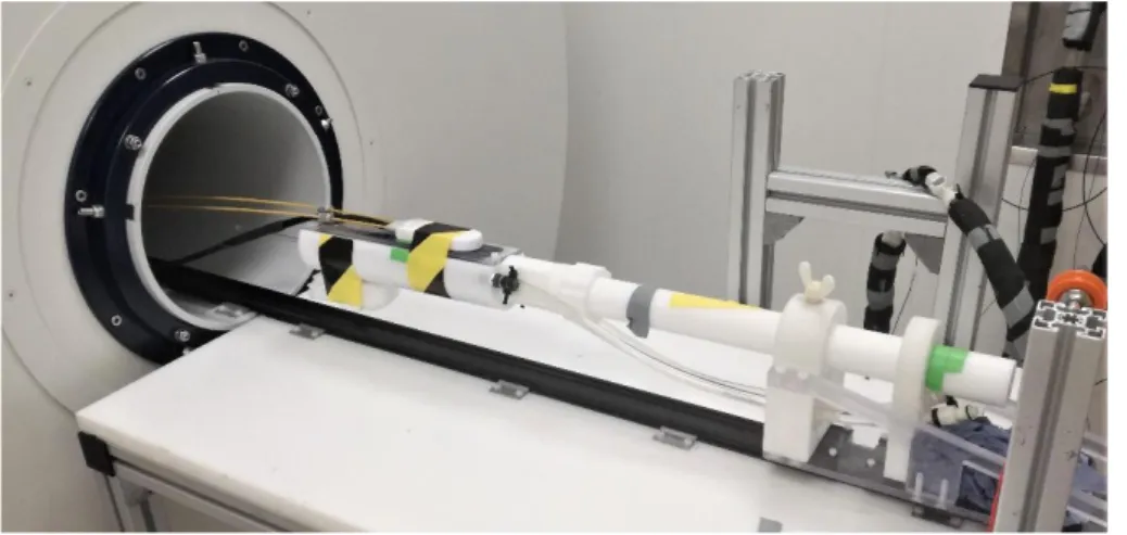
Figure 4-4 Experimental chamber at the positioning device in front of the MRI.
The 31P-NMR surface coil was attached to the upper side of the chamber. The chamber is connected to the seawater cycle by hoses.
Materials & Methods
15 4.4 Nuclear magnetic resonance imaging and spectroscopy
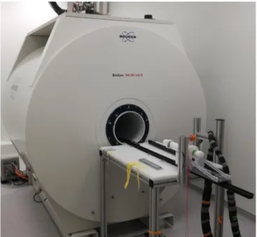
In vivo MRI and 31P NMR spectra were obtained using a 9,4 T animal scanner with a horizontally accessible bore of 30 cm (Bruker Biospin MRI GmbH Ettlingen, Germany, BioSpec 94/30 US/R, AVANCE III) and a BGA‐12S HP B0 gradient system. The signal of the fish was collected with a 2 cm diameter surface coil which was double-tuned for the hydrogen and phosphorous frequencies. The NMR control software (Paravision 6.0.1, Bruker Biospin MRI GmbH) was run on a HP workstation with a Linux based operating system.
Figure 4-5 Photo of the used MRI and positioning device.
94/30 US/R, AVANCE III and in-house built positioning device and insulating tubing for the seawater supply.
4.4.1 Experimental protocol
The experimental chamber was placed into the centre of the MR scanner and the fish was allowed to acclimate to its new setting for 18 hours at least. After control of the position of the animal chamber inside the magnet, consecutive in vivo 31P-NMR spectroscopy scans were conducted over the time course of this post handling phase to control the acid-base and energy status for potential handling-induced alterations.
After an acclimation phase the experimental protocol was started when the fish was considered free of handling stress. Treatment conditions were induced acutely for 24 hours to investigate potential changes in blood distribution, pHi and energetic status of
Materials & Methods
16 brain cells. Finally, after the treatment a control phase of 3 hours was conducted under control conditions. Animals were transported back to the aquaria after the experiment.
All animals survived the MR experiments except for one individual, due to an accidental stop in the water supply during the night.
Over a pre-treatment control phase of 3 hours, the treatment period and a post- treatment control phase of 3 hours in vivo 31P NMR spectroscopy was performed as well as MR imaging. After a tri-pilot scan blocks of three consecutive spectra were followed by a FLASH scan, a BOLD scan and a phase contrast imaging scan. This scheme was repeated over the whole course of the control and treatment phase.
4.4.2 MR imaging and spectroscopy protocol
For the localization of the relevant field of view and for the verification of the fish’s position within the chamber tri-pilot localizer scans were performed to generate an simple MR image giving an 3D overview. The used tri-pilot scans were based on the Bruker Localizer_Service protocol and slightly adapted. For each tri-pilot one scan was conducted with a TE of 4.0 ms and a TR of 100 ms which gave a fast TA of 12 s 800 ms. The slice thickness was 2.0 mm at an image size of 128 x 128 pixels and a field of view of 80 x 80 mm. The excitation pulse was of 1.40 ms length and had a bandwidth of 3000.0 Hz at a FA of 30° and a power of 0.76 W.
The Bruker protocol FLOWMAP was used as base with the reconstruction mode
“VelocityMapping”. The used parameters were a TR of 9.0 ms at TE of 4.0 ms with a FA
of 20° gave a TA of 1m 13s 728 ms duration for one slice and a field of view of 40 x 40 mm and 256 x 256 pixels. 16 averages were generated per scan and anti-aliasing was set to 1.0. The velocity range was set to its minimum of 4.49 cm/s. The excitation pulse used had a length of 0.78 ms, a bandwidth of 5400.0 Hz and a flip angle of 20°and 1.30 W power. Masking threshold was set to 0.0 % after exploratory scans showed very low signal intensities which would make the blood flow in blood vessels masked even under thresholds as low as 0.1 % signal intensity.
RARE scans were used for morphological investigations. The used examination parameters were TR of 1000.0 ms and TE of 40.0 ms and a 90° FA. Eight averages
Materials & Methods
17 were obtained for one slice with a thickness of 1 mm per scan. A field of view of 40 x 40 mm and 256 x 256 pixels were obtained. TA was 2 min 15 s 130 ms.
FLASH scans were used after modifications of the examination parameters to a TR of 85.3 ms. For scans of 0.50 mm slice thickness and 16 averages per scan the TE was set to 10.0 ms with a FA to 60° generated suitable images for morphological analysis and verification of the position of the animal and identification of blood vessels. The acquisition time (TA) was 6 min 33 s 238 ms for a scan with 6. The image size was 256 x 256 pixel for a field of view of 40.0 x 40 mm. The used excitation pulses had a length of 2.0 ms with a bandwidth of 4000 Hz and had a power of 6.45W.
To investigate possible differences in perfusion BOLD MRI scans were used. The used scanning protocol was based on the Bruker T1_FLASH. The parameters used were TE
of 40.0 ms, TR of 100.0 ms with 16 averages resulting in a TA of 7m 40 s 800 ms. For one slice with an image size of 256 x 256 pixels and a field of view of 40.0 x 40.0 mm.
The excitation pulse had a length of 2.0 ms with a bandwidth of 4000.0 Hz and a FA of 60° and a power of 6.45 W.
31P NMR spectroscopy parameters were as follows. The total acquisition time per 31P- NMR spectrum was = 5 min 07 s 200 ms. 256 scans/averages were conducted with a TR of 1200 ms, a FA of 65° and an acquisition duration of 409.6 ms. 4096 acquisition points were used at a acquisition bandwidth of 10000 Hz = 61.70 ppm, a spectral resolution of 1.22 Hz/points and the reference power was 2.714 W. The excitation pulses were bp32 (block pulses) with a length of 0.2 ms, a bandwidth of 6400 Hz and a pulse power of 16.96 W.
4.4.3 Image Analysis
Image analysis was performed in Paravision 6.0.1 (Bruker Biospin MRI GmbH) for phase contrast imaging and in FIJI is just ImageJ (Version 1.52n) for FLASH imaging, BOLD imaging. 3D MIPs were created in HOROS medical image viewer. In the
Materials & Methods
18 obtained MR images regions of interests (ROI) were evaluated either for signal intensity (BOLD and FLASH) or for flow velocity (phase contrast imaging).
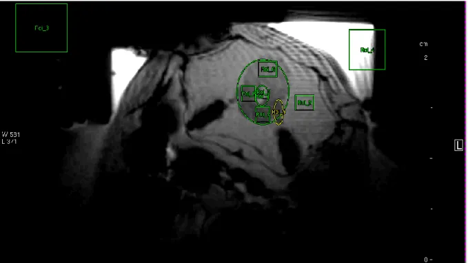
In phase contrast imaging, if the position allowed at least three ROIs were chosen to measure the blood flow in brain vessels while the remaining ROIs were positioned to control for possible aliasing and movement artefacts. They were positioned in areas of the image that represented body tissue, water flow in the surrounding chamber, air outside the chamber and they were positioned according to phase gradient errors due to movement.
Figure 4-6 Example of an axial FLASH scan in vivo with marked ROIs for the evaluation of blood flow.
The NMR spectroscopy analysis workflow consist of several pre-processing steps including a conversion of the free induction decay (FID) to a spectrum in the intensity vs ppm format using a Fourier-transformation in Topspin 3.1PV (Bruker Biospoin GmbH), an automated baseline correction, and manual phase correction. The received
Materials & Methods
19 spectra were calibrated with the peak of PCr to 0 ppm as reference. All in vivo and in vitro calibration spectra were analysed manually.
As indices for the energetic status of the cell metabolism the Pi-PCr-ratio (ratio of the concentration of inorganic phosphate to phosphocreatine) was calculated as well as the signal intensity of βATP which is representative for the ATP level (Borger et al.
1998, van den Thillart 1989).
Materials & Methods
20 4.4.4 Statistical analysis
The data was exported and stored in Microsoft Office 365 Excel sheets. Statistical analysis was carried out using the software R version 3.5.3 (R Core Team, 2019).
Images were obtained, stored and worked on as DICOM (Digital Imaging and Communications in Medicine) files. 31P-NMR spectra were obtained and evaluated using Topspin Software for Paravision 6.0.1. (Bruker Biospin MRI GmbH).
Results
21 5 Results
An experimental protocol was developed to investigate the effects of ocean acidification on the blood distribution and energy metabolism of the brain as well as its intracellular pH (pHi) in Polar cod. The used scanning methodology was refined using a total of 5 fish and applied for experimentation on 2 fish under trial conditions. Different methodologies were tested and compared to investigate the blood distribution of the brain.
5.1 Brain morphology
A series of in vivo morphological scans were conducted on all animals (n = 7). Over the course of this work several MR imaging techniques were tried and compared to produce high quality in vivo MRI brain scans in Polar cod under control and treatment conditions. Different imaging techniques were tried and adapted. Rapid Acquisition with Relaxation Enhancement (RARE) MRI as well as Fast Low Angle Shot (FLASH) MRI scans were tried and compared for morphological imaging. The RARE imaging provided relatively high image contrasts and allowed discrimination between brain regions and surrounding tissues and even between different structures within brain areas. The RARE imaging did not allow the detection of blood flow or blood vessels.
The FLASH imaging in contrast did not provide high contrast and was not very suitable for the discrimination of brain areas and tissues but did exhibit very strong signals even for small blood flows and was therefore suitable to detect blood vessels in the head of the fish and explore the heads vascularity (see Figure 5-1).
Results
22
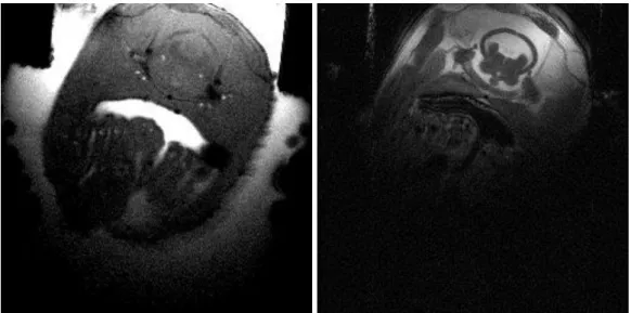
Figure 5-1 Comparison of two different MR imaging techniques.
On the left, there is a FLASH image. On the right there is a RARE image presented. Both images show axial scans (at the same position) through the head of the fish. The images show cross-sections through the fish’s head. In the left image (FLASH) flow is displayed brightly exhibiting water filled mouth cavity and blood flow in the blood vessels of the head, around the brain and around the otoliths, as well as in the gills. In the right image (RARE) the different anatomical structures in the fish’s head can be discriminated by contrast.
Figure 5-2 presents different morphological MR imaging views to illustrate the brain anatomy of Polar cod. Morphological scans of the fishes’ brains and the surrounding head were obtained for the three planes and at different positions.
Figure 5-2 Morphological RARE MRI scans of the brain of polar cod.
(A) coronal plane (B) sagittal plane (C) axial planes at four different positions of the head. The annotated brain regions are I – olfactory nerve, OB – olfactory bulb, Tel - telencephalon, Tec – tectum, EG – eminentia granularis division of the cerebellum, Tel – telencephalon, M – mesencephalon, Di- diencephalon, P – pons, MO – medulla oblongata, CCb –corpus division of the cerebellum, C – Cerebellum. CC – crista cerebellaris of the rhombencephalon
Results
23 5.2 Blood Flow and Perfusion
5.2.1 Vascular morphology
To investigate possible changes in brain perfusion under elevated pCO2 in vivo suitable blood vessels for blood flow investigations had to be found. To find these vessels axial, sagittal and coronal scans were performed. To describe the morphology, distribution of these vessels in the fish head a 3D reconstruction was achieved. Axial scans were used in experiments to find vessels for further investigation using flow-weighted and BOLD MRI techniques.
5.2.2 Angiography scans
Serial axial T1_Flash scans were conducted over the whole length of the animal´s head to find and trace suitable blood vessels for perfusion weighted imaging. For every block of flow-weighted scans T1- weighted scans were repeated to allow the identification of movement and repositioning of the fish.
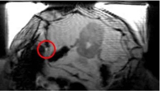
Figure 5-3 Example axial FLASH scan of a Polar cod head.
The image shos a cross-section of the fish head. Obtained for the localisation of blood vessel and neuroanatomical overview. Marked with a red circle a blood vessel is visible as a bright structure.
5.2.2.1 Angiography – Maximum intensity projection (MIP)
For one animal an 3-dimensional angiography model was rendered based on 40 separate time of flight (ToF) angiography scans to display and trace the blood vessels
Results
24 of the fish’s head. As the model is a maximum intensity projection (MIP) blood vessels cannot only be visualized by their signal intensity but also can flow within these be compared by signal intensity representing flow speed with an opacity following a linear table (see Figure 5-4 ff). Movie files of the 3D rendered angiography scans can be found in the digital annex.
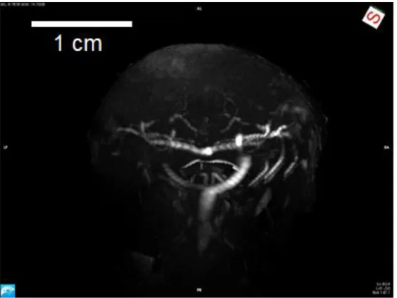
Figure 5-4 3D Angiography MIP axial plane in anterior view.
The 3D model is showing the blood vessels in the fish head. The upper side of the image is dorsal, the lower side ventral. The bright structures are the blood vessels in the head of polar cod. The mouth cavity and the gills were removed digitally.
Results
25
Figure 5-5 3D Angiography MIP in the coronal plane dorsal view.
The 3D model is showing the blood vessels in the fish head. The upper side of the image is caudal, the lower side ventral. The bright structures are the blood vessels in the head of polar cod. The mouth cavity and the gills were removed digitally.
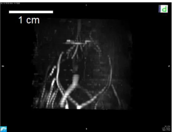
Figure 5-6 3D Angiography MIP sagittal plane.
It is showing the blood vessels in the fish head. The right side of the image is rostral, the left side caudal, the upper side dorsal and the lower side ventral. The bright structures are the blood vessels in the head of polar cod. The mouth cavity and the gills were removed digitally.
Results
26 5.3 In vivo measurement of blood distribution of the brain of polar cod
5.3.1 Method Application
For the in vivo investigation of effects of elevated pCO2 on the blood distribution to the fish’s brain a set of MRI scanning protocols were developed and tested. The methods chosen for the in vivo trials were T1-weighted FLASH scans, BOLD and phase contrast imaging.
5.3.1.1 Phase Contrast MRI
Figure 5-7 example axial phase contrast imaging scans.
On the left a phase contrast angiography reconstruction and a velocity map reconstruction on the right.
Marked in green and yellow are the respective ROIs. The images show the cross-section of the fish. In the left images flow is displayed as bright. The bright areas on top represent water flowing around the fish and the bright areas within the fish represent blood and water in the mouth cavity in the fish. The right image is a velocity map reconstruction of the same scan representing flow velocity and direction by brightness.
Strong aliasing was observed in the top left and top right corner of the images were water was flowing with velocities far beyond the set flow speed in all in vivo scans.
These aliasing effects were not observed within the fish.
Results
27
Figure 5-8 Axial phase contrast imaging scan of fish 6 with ROIs annotated in their respective position.
In fish 6 changes in blood flow could be observed in ROI 1 to ROI 3 comparing control and treatment conditions (see time series plot in Figure 5-9). The ROIs 1 and two were placed laterally over the blood vessels on top of otolith organs. The third ROI was placed over the vessel that lies centrally between them.
The mean blood flow per scan seemed to be relatively stable over the whole trial showing small fluctuations that did not obviously coincide with the treatment. Due to movement of the fish only one phase contrast image could be evaluated for the pre- treatment control of the fish. This scan was compared to 6 scans under treatment conditions before the fish moved again and ROIs had to be re-adjusted.
In ROI 1 the mean blood flow in the first scan before treatment was 0.569 cm/s (standard deviation 0.257) and in the second scan mean blood flow was 0.462 cm/s (standard deviation 0.225). The first scans under treatment conditions showed a flow of 0.149 cm/s (standard deviation 1.470). After that blood flow increased again with 0.253 cm/s (standard deviation 0.673) in the last scan before the fish moved and ROIs had to be adjusted. For the ROIs 2 and 3 the mean blood flow was lower for the first six scans under treatment conditions than in the compared scans under control conditions. For ROI 2 the mean blood flow before treatment was 0.42 cm/s (standard
Results
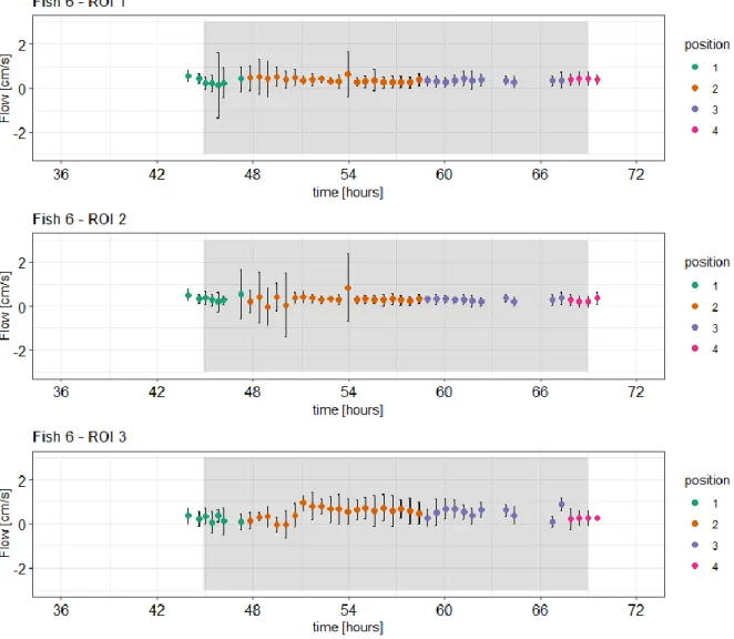
28 deviation 0.098) compared to 0.285 cm/s (standard deviation 0.066) under treatment conditions. For ROI 3 the mean blood flow before treatment conditions was 0.298 cm/s (standard deviation 0.0.074) compared to 0.234 cm/s (standard deviation 0.140) under treatment. To conclude, in all three ROIs the blood flow decreased during the first 1.5 h of treatment conditions compared to the pre-treatment control. In ROI 1 and 2 the blood flow decreased gradually until it reached a minimum at 1 hour after beginning of the treatment and recovered again. For ROI 3 which covered the central vessel no obvious trend was detectable although the mean blood flow also was decreased during the first 1.5 h of treatment
Figure 5-9 Time series of measured blood flow in ROI 1, ROI 2 and ROI 3 in fish 6.
Blood flow was compared for both treatments. The grey areas show the measurement under treatment conditions while the areas with white background show measurements at normocapnic control conditions. The x-axis shows time in hours and the y-axis represents mean blood flow in cm/s the respective ROI with error bars indicating the respective standard deviation. The dots are coloured according to the position of the respective ROI. As it moved at certain occasions over the trial the ROIs had to be adapted accordingly. The time axis starts at zero hours after the end of the acclimation phase when handling stress could be excluded.
Results
29 For fish 7 the same analysis was conducted. Due to repeated movement of the animal over the course of the trial the ROIs had to be rearranged repeatedly to exclude motion artefacts. This led to a division of 7 position for each respective ROI in fish 7 (see time series in Figure 5-10). The ROIs 1, 2, 3, 4, 5, 6 had the shape of circles and were placed over identified as blood vessels in PCA scans. The ROIs 7, 8, 9 and 10 were of rectangular shape and placed to concern for noise and aliasing. Therefore, they were positioned in the area of the image that represents water in the chamber, air around the chamber and tissue of the animal.
The mean blood flow in ROI 1 ranged from 0.040 to 1.61 cm/s with a median of 0.482 cm/s. Before treatment the median in ROI 1 was 0.711 cm/s. After the treatment was administered, the blood flow increased up to 1.61 one hour after treatment began Due to software failure while measuring fish 7 nearly 6 hours of treatment could not be supervised by scans or spectra. Also, in fish 7 unfortunately no blood flow data could be obtained from phase contrast images for the after-treatment control due to strong motion artefacts as the fish was moving repeatedly in this phase. Therefore, the evaluation of possible after-effects could not be performed.
Results
30
Figure 5-10 Time series of measured blood flow in ROI 1, ROI 2 and ROI 3 in fish 7.
The blood flow was compared for both treatments. The grey areas show the measurement under treatment conditions while the areas with white background show measurements at normocapnic control conditions. The x-axis shows time in hours and the y-axis represents mean blood flow in cm/s the respective ROI with error bars indicating the respective standard deviation. The dots are coloured according to the position of the respective ROI. As it moved at certain occasions over the trial the ROIs had to be adapted accordingly. The time axis starts at zero hours after the end of the acclimation phase when handling stress could be excluded.
For the ROIs 4, 6 and 6 which were placed on structures believed to be peripheral blood vessels no effect could be observed. Due to the frequent repositioning of ROIs and the relatively high standard deviations of the measurements in these ROIs the data is inconclusive (see Figure 5-11).
Results
31
Figure 5-11 Time series of measured blood flow from phase contrast imaging in ROI 4, ROI 5 and ROI 6 in fish 7.
Blood flow was compared for both treatments. The grey areas show the measurement under treatment conditions while the areas with white background show measurements at normocapnic control conditions. The x-axis shows time in hours and the y-axis represents mean blood flow in cm/s the respective ROI with error bars indicating the respective standard deviation. The dots are coloured according to the position of the respective ROI. As it moved at certain occasions over the trial the ROIs had to be adapted accordingly. The time axis starts at zero hours after the end of the acclimation phase when handling stress could be excluded.
Results
32 5.3.1.2 Slow Blood Flow Imaging
Figure 5-12 FLASH axial MRI image annotated with ROIs of Polar cod (fish 6) in vivo
In fish 6 seven ROIs were defined. Four of these ROIs were set over the fish brain and three were defined to serve as reference in tissue, air and water to identify possible artefacts. ROI 1 was a polygon covering the whole cross-section of the brain. ROI 2, 3 and 4 were rectangles spread over the brain’s cross-section. Due to movement of the fish positions of the ROIs had to be rearranged three times for fish 6. In ROI 1 there appeared to be slight decrease in signal intensity. In ROI 2 there were no obvious alterations. Over the first 5 hours of treatment there appeared to be an increase in signal intensity in the ROIs 3 and 4 (see Figure 5-13). There were no considerable differences between post-treatment control and treatment conditions.
Results
33
Figure 5-13 Time series of signal intensity from T1-weigthed imaging in ROI 1-4 in fish 6.
Signal intensity was compared for both treatments. The grey areas show the measurement under treatment conditions while the areas with white background show measurements at normocapnic control conditions. The x-axis shows time in hours and the y-axis represents mean blood flow in cm/s the respective ROI with error bars indicating the respective standard deviation. The dots are coloured according to the position of the respective ROI. As it moved at certain occasions over the trial the ROIs had to be adapted accordingly. The time axis starts at zero hours after the end of the acclimation phase when handling stress could be excluded.
In fish 7 the position of the ROIs had to be rearranged 6 times. Position 2 of the ROIs covers the transition from control to treatment with one scan before and on under treatment. In ROI 1-4 no considerable difference in signal intensity could be observed for those scans. Even though, the fish moved, and ROIs had to rearranged, it appears
Results
34 that blood flow differed between one and 5 hours after the treatment was started. In ROI 1 the signal intensity increased after 1.5 h and appeared to be normalized after 4 hours.
Figure 5-14 Time series of measured signal from T1-weigthed imaging intensity in ROI 1-4 in fish 7.
Signal intensity was compared for both treatments. The grey areas show the measurement under treatment conditions while the areas with white background show measurements at normocapnic control conditions. The x-axis shows time in hours and the y-axis represents mean blood flow in cm/s the respective ROI with error bars indicating the respective standard deviation. The dots are coloured according to the position of the respective ROI. As it moved at certain occasions over the trial the ROIs had to be adapted accordingly. The time axis starts at zero hours after the end of the acclimation phase when handling stress could be excluded.
Results
35 5.3.1.3 BOLD Imaging
To investigate possible changes in brain perfusion under ocean acidification BOLD MRI measurements were performed. ROIs were used too analyses of the signal intensities of the images. ROIs were adjusted in size and position if the fish moved. Up to two ROIs were positioned to cover the brain in total with a polygon fitting to its size and three rectangles placed in the ventral, dorsal and on side of the brain to accord for possible effects due to gradients and signal intensity loss due to distance from the surface coil. Additional rectangular ROIs were placed in areas of the image that represented water in the chamber, air outside the chamber and body tissue.
Figure 5-15 BOLD axial MRI image annotated with ROIs of Polar cod (fish 6) in vivo.
In fish 6 four ROIs (ROI 1, ROI 2, ROI 3, ROI 4) were placed over the fish’s brain in axial BOLD imaging to investigate perfusion changes under treatment conditions compared to control conditions. The ROI 1 was fitted to cover the whole cross-section of the brain while ROI 2 and 3 only covered parts of it. ROI 1 was designed to be a polygon covering as much of the brain cross-sections area as possible. ROI 2 and 3 where rectangles only covering a small portion of the brain and were placed in different positions (see Figure 5-15). This should account for possible spatial differences and allow a comparison between the whole cross-section and parts of it. Additional ROIs were placed in the periphery in body tissue, flowing water and air outside the chamber to be able to account for possible artefacts. Due to movement of the fish during control and treatment phase some images could not be evaluated due to motion artefacts. As some of these movements led to a slight change in position of the fish the ROIs had to
Results
36 be adapted to continue covering the respective area. Therefore, six ROI positions had been identified after respective movements.
The first continuous analysis of ROI in fish 6 start at 55 minutes after beginning of the treatment so no control values could be obtained. This position could be analysed for approximately 1.5 hours before the fish started to move again. During these phase the measured signal intensities in the ROI 1 did vary slightly but no trend was observable.
In ROI 2 a strong increase in signal intensity was measured till circa 2h after treatment began. After this peak, a decline seemed to start. In ROI 3 the contrary could be observed as the values decreased. ROI 4 was placed to be outside the chamber. It showed values slightly above zero, which was expected, for all positions except position 2.
Results
37
Figure 5-16 Time series - BOLD in vivo MRI scans of fish 6 in ROI 1- 4 in fish 7.
Signal intensity was compared for both treatments. The grey areas show the measurement under treatment conditions while the areas with white background show measurements at normocapnic control conditions. The x-axis shows time in hours and the y-axis represents mean signal intensities the respective ROI with error bars indicating the respective standard deviation. The dots are coloured according to the position of the respective ROI. As it moved at certain occasions over the trial the ROIs had to be adapted accordingly. The time axis starts at zero hours after the end of the acclimation phase when handling stress could be excluded.