i
Impact of ocean acidification (OA) on the acid-base regulation of polar cod: Time and localized tracking of brain pH changes
Masterarbeit
zur Erlangung des Grades eines
Master of Science (M.Sc.)
Universität Rostock Mathematisch-
Naturwissenschaftliche Fakultät
In Kooperation mit dem Alfred- Wegener-Institut für Polar- und Meeresforschung, Bremerhaven Prof. Dr. Inna Sokolova Dr. Christian Bock
Vorgelegt von Clara Isabella Scheuring September 2019
i Table of Content
List of figures ... i
List of tables ... v
Abbreviations ... v
Zusammenfassung ... ix
Abstract ... x
1 Introduction ...1
1.1 Climate change in the Arctic ocean ... 1
1.2 Polar cod, Boreogadus saida ... 4
1.3 Polar fish in a changing environment ... 5
1.4 pH regulation in fish ... 6
1.5 Magnetic resonance imaging (MRI) and NMR spectroscopy ... 8
1.6 Chemical exchange saturation transfer ... 10
1.7 Hypotheses ... 11
2 Material and Methods ... 12
2.1 Collection of the experimental animals ... 12
2.2 Experimental setup ... 12
2.3 In vivo 31P-NMR spectroscopy ... 14
2.4 CEST measurements... 15
2.4.1 In vitro CEST measurements ... 15
2.4.2 In vivo CEST measurements ... 18
2.5 Statistical analysis ... 19
3 Results ... 19
3.1 In vivo 31P-NMR spectroscopy ... 19
3.2 Energy values ... 22
3.3 pHi regulation ... 23
3.3.1 Fish 1 ... 23
3.3.2 Fish 2 ... 24
3.3.3 Fish 3 ... 24
3.3.4 Fish 4 ... 25
3.3.5 Mean ... 26
3.4 In vivo CEST measurements ... 27
4 Discussion ... 27
4.1 Water chemistry ... 27
4.2 pHi regulation ... 29
4.2.1 in vivo CEST measurements ... 30
4.2.2 Active ion transport as part of pH regulation ... 30
4.2.3 Behavioural changes resulting from pH changes ... 31
4.3 Energy-dependent stress response ... 32
4.4 Fish 1 ... 33
4.5 Comparison of CEST and in vivo 31P-NMR spectroscopy ... 33
4.6 Conclusions ... 35
4.7 Perspectives ... 36
Bibliography ... 37
Appendix ... 52
Acknowledgements ... 56
Declaration ... 56
i List of figures
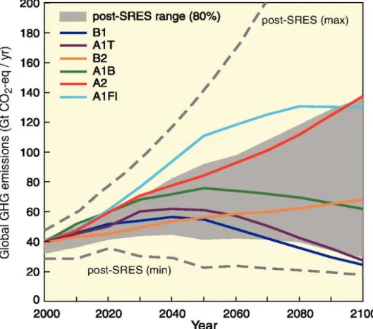
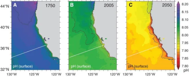
Figure 1: Global Greenhouse gas (GHG) emissions (in GtCO2-equivalent per year) in the absence of additional climate policies: the special report on emission scenarios (SRES) A1B, A1Fl, A1T, A2, B1 and B2 (coloured lines) and 80th percentile range of recent scenarios published since SRES (post-SRES) (grey shaded area). Dashed lines show the full range of post-SRES scenarios. The GHG emissions include CO2, CH4, N2O and F-gases. www.ipcc.ch AR4 Report ... 2 Figure 2: Evolution of the water pH off the coast of California from 1750 until 2050.
C shows the predicted decrease in ocean pH for the A2 IPCC scenario (Gruber et al. 2012). ... 3 Figure 3: (a) Map of average bottom water temperature between 1985 and 2004 in
the arctic ocean and (b) a trend in the next 100 years under CO2 increase.
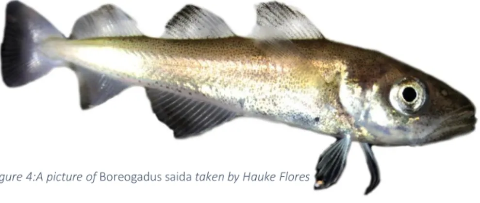
Acronyms mark the Arctic Ocean (AO), European Nordic Seas (ENS), Barents Sea (BS) and the Laptev Sea (LS) ... 4 Figure 4: A picture of Boreogadus saida taken by Hauke Flores ... 5 Figure 5: Model of the GABAAR to show hypercapnia-induced changes published by
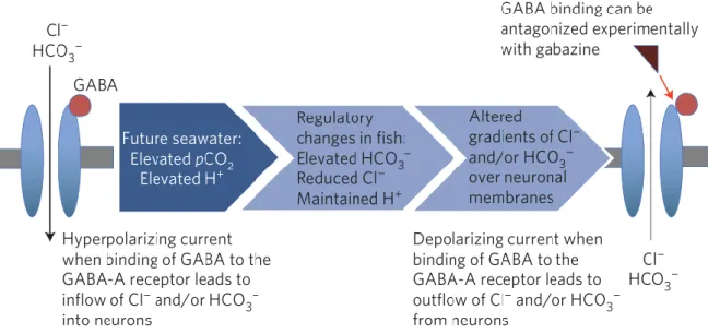
Nilsson et al. 2012. Normally functioning GABAAR (left) leading to a hyperpolarisation of the cell by an Cl-/ HCO3- inflow after GABA binding. A GABAAR in a gabazine treatment (right) leading to a depolarisation of the cell by a Cl-/ HCO3- outflow. ... 8 Figure 6: Technical drawing of the brain of B. saida with the olfactory tract (olt),
olfactory bulb (OB), telencephalon (Tel), optic tectum (Tec), Cerebellum (C), cerebellar crest of the rhombencephalon (CC) and spinal cord (SC).
Identification of the brain regions according to Ou & Yamamoto 2016 and Kawaguchi et al. 2019 ... 9 Figure 7: Brain regions of polar cod on MRI scans with OB, Tec, Tel, C, CC, eminentia
granularis (EG), Corpus division of the Cerebellum (CCb), Mesencephalon (M), Diencephalon (Di), Pons (P) and Medula oblongata (MO) ... 9
ii
Figure 8: The principle of CEST is illustrated above. Protons of a solute being saturated by a specific RF. Saturated protons of the solute then exchange with water protons, thereby decreasing the water signal proportional to the solute concentration. Modified illustration by Wermter (2017) ... 10 Figure 9: A: Testing chamber with the experimental animal inside and tubes with
water inflow (a) and outflow (b). Dental wax helps to position the fish at the frontal part of the chamber. B: Schematic design of the experimental setup with the heater tanks H1 (normocapnia) and H2 (hypercapnia), water inflow (A), water outflow (B) in an isolated tube (D), the experimental camber (E) and the MRT (F). ... 12 Figure 10: in vivo MR image of the head of B. saida obtained with a 1H/13C resonator
with an inner diameter of 72 mm. The yellow circle marks the area sensitive to the 31P-NMR-surface coil. ... 15 Figure 11: Phantom tube with different pH values of the same solution in the NMR
tubes for the in vitro CEST study. ... 15 Figure 12: Experimental design of the in vitro study with A: heater tank; B: water hose;
C: isolation; D: NMR tubes with testing solution; E: magnet resonance tomograph. On the left the realistic proportions are shown. ... 16 Figure 13: MR image of a phantom with a different pH value (6.5; 6.8; 7.0; 7.2; 7.5;
7.8) in every tube. The yellow circles show the chosen ROI that was evaluated first in Fiji image J and then in MATLAB. ... 17 Figure 14: Z-spectra showing the CEST effect in percent for a chemical shift of 1 ppm
and 2.8 ppm. In A with a high CEST effect and in B no CEST effect. A shows the CEST effect for TMAO at 15 °C at a pH of 7. B shows the CEST effect for BSA at 5°C at a pH of 7.5... 17 Figure 15: The CEST effect for a chemical shift of 1 ppm in A (BSA) and C (TMAO) and
for a chemical shift of 2.8 ppm in B (BSA) and D (TMAO). TMAO shows a CEST effect for δ 1ppm at a pH of 6.5 and a temperature of 10°C and 15°C. ... 18
iii
Figure 16: Testing slice for the in vivo CEST measurements with the chosen ROI in the yellow box. The MRI scan was obtained with a 1H/13C resonator with an
inner diameter of 72 mm. ... 18
Figure 17: Typical in vivo 31P-NMR spectrum showing relative concentrations of phosphometabolites in a brain cell of B. saida. Phosphometabolites in the brain are sP = sugar Phosphates; cAMP = cyclic AMP; Pi = inorganic Phosphate; PCr = Phosphor creatine and the three phosphate groups γ-, α- and β-ATP. The PCr peak was set to 0 ppm. The other metabolites have a chemical shift in ppm in relation to PCr. ... 19
Figure 18: Two 31P-NMR spectra showing a different chemical shift of Pi in relation to PCr. The difference in δ between the two displayed spectra is 0.11 ppm. ... 20
Figure 19: Stacked 31P-NMR spectra of A: two hours of control conditions before switching to hypercapnia. B: the first two hours of hypercapnic conditions and C: the recovery time under normocapnic conditions after hypercapnia. The stacked spectra show the fluctuations in the signal intensity of the phosphometabolites. The acquisition of every spectrum takes five minutes. The displayed spectra were acquired in experiments with Fish 3. ... 21
Figure 20: The energy values of every fish indicated by the Pi/PCr ratio, given in relative units [ru], and displayed in A-D. A comparison of all fish is shown in E. Time 0 is 3 hours before switching to hypercapnia. ... 22
Figure 21: pHi and pHw of fish 1 during the experiment. Since pHw was especially low on this experiment day it is plotted separately (red line). ... 23
Figure 22: pHi and pHw of fish 2 during the experiment. ... 24
Figure 23: pHi and pHw of fish 3 during the experiment. ... 25
Figure 24: pHi and pHw of fish 4 during the experiment. ... 25
Figure 26: Boxplots of all datapoints in the three different treatments with a significant difference (p-value < 0.001) of the datapoints during hypercapnia compared to the control and normocapnic datapoints. ... 26
Figure 25: pHw and a mean pHi of fish 2, 3 and 4 during the experiment. ... 26
iv
Figure 27: A: The changing CEST effect in vivo, over time, evaluated for 1 ppm and 2.8 ppm. Every datapoint represents the mean value of three CEST measurements. The CEST results show a higher effect during hypercapnia for a chemical shit of 1 ppm as well as for 2.8 ppm. B: Mean values for the control (blue) as well as the hypercapnic (red) treatment evaluated for 1 ppm and in C: 2.8 ppm. Both graphs show a higher CEST effect during hypercapnia than during the control.. ... 27 Figure 28: water pH of both H1 and H2 during the whole time of the experiment. Areas
underlaid in red are actual experiment days were 31P-NMR scans on B. saida were performed. ... 28 Figure 29: pCO2 of both the normocapnic water reservoir and the hypercapnic water
reservoir during the whole time of the experiment. The striven pCO2 values for the normocapnic tank was 500 ppm and for the hypercapnic tank 3500 ppm. ... 28 Figure 30: Stacked 31P-NMR spectra of two hours of control conditions before
switching to hypercapnia in the experiment in fish 1. ... 53 Figure 31: Stacked 31P-NMR spectra of one hour of control and one hour of
hypercapnia in the red box in the experiment with fish 1... 53 Figure 32: Stacked 31P-NMR spectra of the first two hours of hypercapnic treatment in
the experiment with fish 1. ... 53 Figure 33: Stacked 31P-NMR spectra of the last two hours of hypercapnic treatment in
the red box and then the normocapnic treatment outside the red box for the experiment with fish 1. ... 54 Figure 34: The CEST effect for BSA and TMAO evaluated at 2.8 ppm on a smaller scale.
The CEST Effect is again higher for TMAO than for BSA. ... 54 Figure 35: Shown here are the first hours after placing the experimental animal in the
testing chamber. A: Mean values for fish 1, 2, 3 and 4. B: Mean value for fish 2, 3 and 4.C-F show the values for each fish alone. ... 55
v List of tables
Table 1: Seawater chemistry of the control (H1) and the hypercapnic (H2) water reservoirs. Temperature, salinity, pCO2, pHw, Total alkalinity and dissolved inorganic carbon were measured and HCO3- was calculated via CO2Sys macro for Microsoft excel (v2.1). ... 14 Table 2: Three different approaches for the in vitro CEST measurement. One
negative control only consisting of PBS. One solution with PBS and BSA [10 mM] and one solution with PBS and TMAO [10mM]. Chemicals with the used concentrations to produce PBS are listed below. All solutions were adjusted to the following pH values: 6.5; 6.8; 7.0; 7.2, 7.5 and 7.8 and tested at seven different temperatures. ... 16 Table 3: Scan properties of all performed NMR scans in this study (31P-NMR
spectroscopy, in vitro CEST and in vivo CEST measurements). ... 52
Abbreviations
ANOVA Analysis of variance
AO Arctic ocean
aq Aqueous
ATP Adenosinetriphosphate
B. saida Boreogadus saida
BS Barents Sea
BSA Bovine serum albumin
C Cerebellum
CaCO3 Calcium Carbonate
cAMP Cyclic Adenosine monophosphate
CC Cerebellar crest of the rhombencephalon
CCb Corpus division of the cerebellum
CEST Chemical exchange saturation transfer
Cl- Chloride
vi
cm Centimetre
CO2 Carbon dioxide
CO32– Carbonate
13C Carbon isotope with mass number 13
D Diencephalon
δ Chemical shift
DIC Dissolved inorganic carbon
DMO 5,5-dimethyl-2,4-oxazolidinedione
DOM Dissolved organic matter
EG Eminentia granularis
ENS European Nordic seas
Eq Equivalent
fig Figure
FISP Fast imaging with steady state precession
FOV Field of view
g Grams
GABA Gamma amino butyric acid
GABAAR Gamma aminobutyric acid type A receptor
GHG Greenhouse gas
Gt Giga tons
h Hour(s)
HCO3- Hydrogen carbonate
ht Header tanks
H2O Water
1H Hydrogen isotope with mass number 1
IPCC Intergovernmental Penal on Climate Change
K+ Potassium
KCl Potassium chloride
KH2PO4 Potassium dihydrogen phosphate
LS Laptev Sea
vii
M Mesencephalon
mm Millimeter
mM Millimolar
mmHg Millimetre of mercury
MO Medulla oblongata
MRI Magnetic resonance imaging
MRT Magnetic resonance tomograph
ms Milliseconds
NaCl Sodium chloride
Na2HPO4 * 2H2O Disodium hydrogen phosphate dihydrate
NMR Nuclear magnetic resonance
OA Ocean acidification
olt Olfactory tract
P Pons
PBS Phosphate buffered saline
PCr Phosphocreatine
pCO2 Partial pressure of CO2
Pd Phosphodiester
pH -log10[H+]
pHe Extracellular pH
pHi Intracellular pH
pHw Water pH
Pi Inorganic phosphate
ppm Parts per million
31P Phosphorous isotope with mass number 31
RARE Rapid acquisition with relaxation
enhancement
RF Radio frequency
ROI Region of interest
ru Relative units
viii
SC Spinal cord
sP Sugar phosphate
SRES Special report on emission scenarios
T Tesla
TA Total alkalinity
TauCEST Chemical exchange saturation transfer from
taurine to water
TE Echo time
Tec Tectum
Tel Telencephalon
TO Optic Tectum
TR Repetition time
TMAO Trimethylamine N-oxide
W Watt
Ø Diameter
% Percent
ix Zusammenfassung
Durch Kohlenstoffdioxid (CO2), das sich in der Atmosphäre akkumuliert, verändert sich unser Klima, was zum globalen Klimawandel führt. Das CO2 löst sich zudem im Ozean, wo es den pH- Wert des Wassers reduziert und zu einer Ozeanversauerung (OA) führt. Lange wurde davon ausgegangen, dass Fische von dieser Versauerung nicht betroffen wären, da sie über eine effektive Säure-Base Regulation verfügen. In den letzten Jahren wiesen jedoch verschiedene Studien darauf hin, dass eine Reduktion des pH-Werts Verhaltensänderungen und Veränderungen in neurologischen Prozessen herbeiführen kann. Um die Säure-Base Regulation im Gehirn des Polardorschs (Boreogadus saida) zu untersuchen, wurden in dieser Studie zwei Methoden, die auf dem Phänomen der Nuklearen Magnetischen Resonanz (NMR) beruhen, kombiniert. Mit nicht-lokalisierter 31P-NMR Spektroskopie konnte die Konzentration verschiedener Phosphormetabolite bestimmt werden. Mithilfe von 31P-NMR Spektroskopie können kurzzeitige Änderungen der Konzentrationen der Phosphormetabolite und damit kurzzeitige Änderungen des intrazellulären pH (pHi) bestimmt werden. Der pHi wurde aus der chemischen Verschiebung des Signals von anorganischem Phosphat zu Phosphorkreatin bestimmt. Da nicht-lokalisierte 31P-NMR Spektroskopie allerdings nicht den pH in einem Areal von der Größe eines Fischhirns bestimmen kann, sollten über den Sättigungstransfer einer chemischen Verschiebung (chemical exchange saturation transfer (CEST)) ortsaufgelöst pH- Änderungen verfolgt werden. CEST ist eine Bildgebungsmethode, die den Austausch zwischen den Protonen des Wassers mit austauschbaren Protonen von Metaboliten detektiert, wie zum Beispiel Taurin (TauCEST) im Gehirn von B. saida. Der CEST Effekt ist unter anderem pH abhängig und kann somit Änderungen im pHi ortsaufgelöst über das Gehirn aufzeigen.
Zusätzlich zu pH Änderungen wurde der Energiestoffwechsel von B. saida unter akuter Versauerung mittels 31P-NMR Spektroskopie analysiert. 31P-NMR Spektroskopie misst die Konzentration von anorganischem Phosphat, Phosphorkreatin und den drei ATP Untereinheiten α-, β- und γ-ATP. Nach 20 Stunden Akklimatisierung unter Kontrollbedingungen wurden die Fische für vier Stunden einer CO2 Konzentration von 3500 ppm (Hyperkapnie) und einem Wasser pH von 6.92 ± 0.2 ausgesetzt. Danach wurden die Fische wieder unter Kontrollbedingungen untersucht (pH 7.96 ± 0.3). Nach Umschalten auf Hyperkapnie sank der pHi im Mittel um 0.5 ± 0.2 pH-Einheiten. Bei zwei Fischen lag die maximale Reduktion des pHi
bei 0.17 pH-Einheiten. Signifikante Veränderungen im Energiestoffwechsel konnte bei keinem Tier festgestellt werden.
x Abstract
A consequence of accumulating carbon dioxide (CO2) in the atmosphere is global climate change. CO2 also dissolves in the ocean and reduces the water pH, resulting in ocean acidification (OA). Fish were long thought to be relatively resistant to pH changes in the water, because they possess an efficient acid-base regulation. However, recent findings indicate altered behaviour and changes in neurological processes in fish. To investigate the acid-base regulation in the brain of the polar cod (Boreogadus saida), a combination of two methods, based on the nuclear magnetic resonance (NMR) phenomenon, was used in this study. Non- localized 31P-NMR spectroscopy was used to measure the concentration of phosphometabolites. The intracellular pH (pHi) was calculated from the chemical shift of the NMR signal of inorganic phosphate in relation to the phosphocreatine signal. 31P-NMR spectroscopy is used to detect short-term changes in the concentration of different phosphometabolites and hence short-term changes in the pH. However, the determination of the pH value in a specific region as small as the fish brain is not possible with non-localized 31P- NMR spectroscopy. To verify the results of the measurements the chemical exchange saturation transfer (CEST) between taurine and water (TauCEST) was determined in a specific region in the brain of B. saida. Because CEST is pH dependant, changes in the CEST effect can give evidence on any pH changes with a higher spatial resolution than non-localized 31P-NMR spectroscopy. Additionally to pH changes, energy metabolism can be analysed with 31P-NMR spectroscopy by measuring the concentration of phosphometabolites such as inorganic phosphate, phosphocreatine or the three ATP subunits α-, β- and γ-ATP. After 20 hours of acclimatisation under control conditions, the animals were exposed to a CO2 concentration of 3500 ppm and a water pH of 6.92 ± 0.2 for four hours (hypercapnia). Then, the animals were tested again in water without elevated CO2 concentrations (pH 7.96 ± 0.3). The pHi decreased rapidly after switching to hypercapnia by a mean of 0.05 ± 0.2 and started to reach control values again after two hours. The maximum decrease in pHi was 0.17 and occurred in fish 2 and 4. Throughout the whole time of the experiment, there were no significant changes in the energy values.
1 1 Introduction
1.1 Climate change in the Arctic ocean
The ocean plays a major role in regulating the Earth’s climate, since it absorbs over 25% of the atmospheric carbon dioxide (CO2) and 90% of the heat that accumulates in the atmosphere (Gattuso 2015). Through anthropogenic effects and the Industrial Revolution, atmospheric partial pressure of CO2 (pCO2) rose from 280 ppm before the Industrial Revolution to a maximum of 413.9 ppm in 2019, leading to a global climate change (Bijma & Burhop 2010, https://www.co2.earth/daily-co2). Atmospheric CO2 levels are predicted to rise to 750 – 1000 ppm by the end of the century (Pörtner 2008, Meinshausen et al. 2011). Three major stressors are associated with climate change: warming, deoxygenation and acidification, all affecting marine ecosystems and their productivity (Bopp et al. 2013, Popova et al. 2016). As temperature in the oceans rises, marine ecosystems suffer from many negative impacts, including mass mortality of marine invertebrates due to heat stress, shifts in the distribution of marine species and associated structural changes in marine communities (Oliver et al. 2017, 2018). Rising temperature in Arctic environments leads to melting sea ice, posing a problem for many marine organisms, who depend on the sea ice (Chambault et al. 2018). Temperature strongly affects exothermic organisms, including fish (Boscolo-Galazzo et al. 2018).
Another aspect of global climate change is ocean deoxygenation (Gómez1 et al. 2018, Junium et al. 2018). Global warming decreases the solubility of gases in the seawater leading to less dissolved oxygen in the open ocean (Gilbert & Rabalais 2010, Popova et al. 2016). With oxygen levels below 2 mll-1 the ecosystem is defined as hypoxic (Diaz & Rosenberg 1995). Benthic organisms evolved tolerance mechanisms to hypoxia, but fish are more sensitive to decreasing oxygen concentrations and mass mortality has been reported (Diaz & Rosenberg 1995).
Besides ocean warming and expanding hypoxia, global climate change leads to another problem, referred to as ocean acidification (OA) ( Caldeira & Wickett 2003, Melzner et al. 2009, Bozinovic & Pörtner 2015). The atmospheric CO2 dissolves in the ocean and when it dissociates, hydrogen ions are being released (according to the following formula), which results in a lower pH (Orr et al. 2005, Bijma & Burhop 2010).
CO2 + H2O ↔ H2CO3 ↔ H+ + HCO3- ↔ 2H+ +CO32-
The current pH in the seawater surface is around 8.05, but by absorbing the atmospheric CO2,
the pH of the seawater decreases as it has already by 0.1 units compared to pre-industrial times [1]
2
(Orr et al. 2005, Gruber et al. 2012, Wermter et al. 2018). Moreover, it is expected to decrease up to 0.77 units by 2300 due to global climate change (Caldeira & Wickett 2003, Heuer & Grosell 2018).
To which extent global climate change will affect these processes depends on emission scenarios (Caldeira &Wickett 2005). There are six different scenarios of future CO2 emissions, as well as other greenhouse gas emissions estimated by the intergovernmental panel on climate change (IPCC). Three scenarios belong to the A1 storyline and estimate very rapid economic growth, a peak in global population development in the mid-century and are distinguished by different technologies used in the energy system. The A2 storyline describes a continuously increasing global population, slower changes in technologies and primarily regional economic development. This scenario shows the highest long-term greenhouse gas emissions and is the one closest to reality at the moment (IPCC 2014). The technology changes in the B2 scenario are more diverse and sustainable than in all the other scenarios. Global population growth is also continuously increasing but not as fast as in the A2 scenario (IPCC 2000). The least long-term greenhouse gas emissions are estimated in the B1 scenario that
Figure 1: Global Greenhouse gas (GHG) emissions (in GtCO2-equivalent per year) in the absence of additional climate policies: the special report on emission scenarios (SRES) A1B, A1Fl, A1T, A2, B1 and B2 (coloured lines) and 80th percentile range of recent scenarios published since SRES (post-SRES) (grey shaded area). Dashed lines show the full range of post-SRES scenarios. The GHG emissions include CO2, CH4, N2O and F-gases. www.ipcc.ch AR4 Report
3
describes a rapid change in energy technologies towards clean and sustainable methods and the same population growth as described in the A1 scenario. All six emission rate scenarios are illustrated in figure 1. Estimated changes in the future ocean pH at the Bay of California according to the high-emission A2 scenario are shown in figure 2 by Gruber et al. (2012).
Biastoch et al. (2014) predict a pH decrease of 0.25 units in the Arctic ocean within the next 100 years. Not only does the ocean pH decrease with rising CO2 concentrations in the atmosphere, but also the concentrations of carbonate (CO32–) in the ocean decreases as
CO2[aq] increases, according to formula 1 (Orr et al. 2005, Kroeker et al. 2013). This makes it difficult for marine calcifying organisms like corals or bivalves to form biogenic calcium carbonate (CaCO3), which results in deformed shells or lowered calcification rates (Kroeker et al. 2013, Liu et al. 2018). Therefore, many studies have been done on the effects of OA on calcifying organisms (Orr et al. 2005, Kroeker et al. 2013, Boch et al. 2018, Zittier et al. 2018).
Temperature and pH changes occur faster in polar regions than in other environments (Field et al. 2018, Zittier et al. 2018). As seen in figure 4, the mean bottom water temperature in the Barents Sea is between 2 - 5°C (Fall et al. 2018, Petrini et al. 2018). It has already increased by about 3°C compared to 1985, whereas the global average temperature has only increased by 1°C (Hassol 2004). It is predicted that Arctic sea surface temperatures will rise by about three times the global average (Praetorius et al. 2018). This so called Arctic amplification is a result of weather events like clouds, surface albedo and poleward oceanic and atmospheric heat transport (Praetorius et al. 2018). Global warming and ocean acidification affect all marine habitats, but since organisms in the polar oceans are adapted to a narrow temperature range, both processes pose an especially great threat to these habitats and their inhabitants (Kroeker
Figure 2: Evolution of the water pH off the coast of California from 1750 until 2050. C shows the predicted decrease in ocean pH for the A2 IPCC scenario (Gruber et al. 2012).
4
et al. 2013, Gattuso et al. 2018, Wermter et al. 2018). Moreover, marine populations are projected to move poleward, leading to the occurrence of invasive species in higher latitudes (Turingan & Sloan 2016, Wilson et al. 2016, Monllor-Hurtado et al. 2017).
1.2 Polar cod, Boreogadus saida
The polar cod (Boreogadus saida; Lepechin, 1774 (fig. 5)), a pelagic, schooling fish, one of the most abundant fish species in the Arctic and subarctic waters, is an important polar organism, because it links several trophic levels (Welch et al. 1992). It reaches a size of up to 46 cm (see Hop & Gjøsæter 2013 for review) while the mean size is 30 cm with a weight of 33 g (Scott &
Scott 1988, Welch et al. 1992). The maximum age is found to be seven years, but rarely exceeds the age of five (Bradstreet et al. 1986, Hop et al. 1997, Ajiad et al. 2011). Schools of adult polar cods have been found under the sea ice as well as in the open water during summer (Crawford
& Jorgenson 1990, Hop et al. 1997). The polar cod feeds on copepods living directly under the sea ice surface and hence lives in close association with the sea ice (Lønne & Gulliksen 1989).
The polar cod itself is an important prey for seabirds and marine mammals, such as the white whale (Delphinapterus leucas, Pallas, 1776), the narwhal (Monodon monoceros, Linnaeus, 1758) and the ringed seal (Pusa hispida, Schreber, 1775) because of its high lipid/energy
Figure 3: (a) Map of average bottom water temperature between 1985 and 2004 in the arctic ocean and (b) a trend in the next 100 years under CO2 increase. Acronyms mark the Arctic Ocean (AO), European Nordic Seas (ENS), Barents Sea (BS) and the Laptev Sea (LS)
BS BS
(Biastoch et al. 2014).
5
content (Welch et al. 1992, Kühn et al. 2018, Landry et al. 2018). Therefore, B. saida is responsible for a major part of the energy transfer from primary and secondary production to higher trophic levels in the arctic ecosystem (Welch et al. 1992, Hop & Gjøsæter 2013). B. saida lives in water temperatures that range from -2°C in winter up to 8°C in summer (Drost et al.
2014). However, its temperature preference has been determined experimentally to be at 3 – 4°C (Christiansen et al. 1996). The distribution in water temperature below the thermal optimum is most likely due to reduced competition as well as special adaptations (Hop &
Gjøsæter 2013). As part of the arctic ecosystem B. saida is adjusted to constant low temperatures and as an example has antifreeze glycoproteins (Zhuang et al. 2012). Cattano et al. (2018) discovered that pelagic species, like B. saida, are more likely to die from high CO2
levels than benthic species. This may be due to more stable CO2 concentrations in the open ocean, whereas at the ocean bottom CO2-levels naturally fluctuate (Hofmann et al. 2011, Munday et al. 2011, Murray et al. 2014). Therefore, it is crucial to investigate any effects of OA and global warming on B. saida to gain knowledge and make predictions on the whole Arctic ecosystem concerning global warming (Kühn et al. 2018, Landry et al. 2018).
1.3 Polar fish in a changing environment
Temperature is a driver in species distribution and population structures (Pörtner et al. 2008).
Rising temperatures are predicted to shift species distributions towards the poles (Perry et al.
2005). With climate change the distribution and abundance of B. saida is declining in the Barents Sea, whereas its boreal relative, the Atlantic cod (Gadus morhua, Linnaeus, 1758), shifted its distribution poleward (Decamps et al. 2017). Diet content is considered to differ between the two species hence no evidence for prey competition was found (Renaud et al.
2012). However, a possible predation of G. morhua on B. saida has been suggested (Renaud et al. 2012). A major impact climate change has on the Arctic ecosystem, namely B. saida, is the decreasing sea ice. Since spawning for B. saida is reported during winter under the sea ice, this
Figure 4:A picture of Boreogadus saida taken by Hauke Flores
6
threatens its reproduction (Craig et al. 1982). Kunz et al. (2016) investigated different parameters such as growth rate and thermal optimum for both B. saida and G. morhua under climate change conditions. Their findings suggest a slower growth rate of 0.39% d-1 for B. saida than for G. morhua, which showed a growth rate of 0.82% d-1. G. morhua also showed a higher tolerance to projected future pCO2 values than B. saida (Kunz et al. 2016).
The current temperature trend goes hand in hand with a decreasing ocean pH and OA (Pörtner et al. 2004). Additionally, OA also results in a reduction of the surface water oxygen level, which may affect the degree of sensitivity of an organism to other environmental factors (Pörtner et al. 2005). Organisms living in an environment with elevated CO2 levels have elevated energy costs (Ishimatsu et al. 2008). However, costs for energy-dependent metabolic processes can be minimalised by specialising on a narrow temperature range as appearing in polar regions (Pörtner 2006). During acute respiratory acidosis from OA, reductions in extracellular blood pH (pHe) and intracellular pH (pHi) have been observed (Pörtner et al. 2005, Shartau et al. 2016).
Influences on the energy budget affect physiology, development and behaviour (Nilsson et al.
2012, Heuer & Grosell 2016, 2018).
1.4 pH regulation in fish
Fish were long thought not to be as sensitive to elevated CO2 levels and pH changes as marine invertebrates, because of their effective acid-base regulation and the higher regulatory capacity of ion exchange (Claiborne et al. 2002, Melzner et al. 2009, Pörtner et al. 2011, Cattano et al. 2018). As well as controlling their pHi through active ion transport, fish have epithelia which limit ion losses, because ions can only pass the membrane through specific channels (Pörtner et al. 2005). However, they react to elevated CO2 partial pressure (pCO2) (hypercapnia) by increasing their ventilation rate (Pörtner et al. 2005), reducing protein synthesis (Langenbuch & Pörtner 2017), behavioural disturbances (Schmidt 2019), metabolic depression (Pörtner et al. 2004) and eventually cardiac failure (Ishimatsu et al. 2004). Even higher mortality was discovered in fish that have been exposed to long term elevated CO2 concentration, but the exact reasons remain unknown (Ishimatsu et al. 2008). When the intracellular pH drops, fish excrete H+ ions across the gills, kidney and intestine as a countermeasure (Ishimatsu et al.
2008, Heisler 1986). The gill epithelium is the first regulatory site, therefore being the main epithelium for acid-base transfer to the water (Claiborne et al. 2002). The pH homeostasis in the brain is provided by transporting or buffering of acid equivalents (Sinning & Hübner 2013).
7
With acid-base relevant ions like chloride (Cl-) or bicarbonate (HCO3-), fish regulate and maintain their tissue pH (Chung et al. 2014). However, during hypercapnia the CO2 equilibrium is shifted, according to formula 1, towards HCO3- and H+ (Shartau et al. 2016). This equilibrium shift lowers the internal pH and results in acidosis (Shartau et al. 2016). Previous studies showed that a decreasing pH in the brain leads to a decrease in the rate of synaptic vesicle release which ultimately results in a limited excitability of the brain (Sinning & Hübner 2013, Wermter et al. 2018). Brain pH changes indicate neurological as well as behavioural disorders through disturbances in the acid-base balance of the organism (Wermter et al. 2018, Schmidt 2019). The gamma-aminobutyric acid type A receptor (GABAAR) is a Cl- and HCO3- channel, activated by the neurotransmitter GABA (gamma amino butyric acid) (see for instance Schmidt et al. 2018). After GABA binding, the channel allows Cl- and HCO3- to pass the cell membrane, resulting in a hyperpolarization and causing less neuronal activity (Chung et al. 2014).
Therefore, a decreasing pH leads to a decreasing neuronal activity, whereas an increasing pH leads to an increasing neuronal activity (Sinning & Hübner 2013). During high CO2 exposure the membrane gradients of Cl- and HCO3-, and therefore, the GABAAR function, is disturbed (Chung et al. 2014). This disturbance leads to a slower reaction of the animal (Chung et al. 2014). In addition to this, Chivers et al. (2014) found that fish cannot process sensory information during CO2 exposure. This matches the results of Ferrari et al. (2012), suggesting that the visual system is affected by high CO2 concentrations. Therefore, pHi regulation in the brain is very important.
When exposed to CO2 and then treated with the GABAAR blocker gabazine, the effects of CO2
can be neutralized as shown in figure 5 (Nilsson et al. 2012, Chung et al. 2014, Munday et al.
2016).
8
1.5 Magnetic resonance imaging (MRI) and NMR spectroscopy
Magnetic resonance imaging (MRI) and nuclear magnetic resonance (NMR) spectroscopy can give insight into the neurological processes in the brain of an animal (Schmidt et al. 2014). These techniques are non-invasive and do not use harmful radiation, but radio frequency (RF) and are, therefore, a useful method for repeatedly gaining information about the intact, living organism (Lee et al. 2010). Metabolism and stress responses can be followed directly in various tissues (Van den Thillart et al. 1989, Lee et al. 2010). Both techniques are based on the physical phenomenon of NMR (Bloch 1946, Purcell et al. 1946). An object in the magnetic resonance tomograph (MRT) is exposed to a very strong magnetic field leading, to a polarisation of the nuclei (Schild 1990). This polarisation is referred to as longitudinal magnetisation along the external magnetic field (Schild 1990). The nuclei commonly used for MRI and MRS are either protons (1H) or other nuclei, such as phosphorous (31P) or carbon (13C) (Lee et al. 2010, Pritchard
& Flemming Hansen 2019). Then, the RF is applied and absorbed by the nuclei, causing the nuclei to point in one direction, the transverse direction (Schild 1990). The RF decreases longitudinal magnetisation and builds up transversal magnetisation (Schild 1990). Depending on the choice of nuclei, the RF needs to be adjusted, because different nuclei absorb different RF (Schild 1990). When the RF is switched off, the system returns to its relaxed state and resonance frequency is emitted during this relaxation (Schild 1990). Nuclei in different tissues vary in relaxation time which leads to different contrasts in the MRI (Schild 1990). NMR spectroscopy determines the chemical shift that occurs when the nucleus emits modulated
Figure 5: Model of the GABAAR to show hypercapnia-induced changes published by Nilsson et al. 2012. Normally functioning GABAAR (left) leading to a hyperpolarisation of the cell by an Cl-/ HCO3- inflow after GABA binding. A GABAAR in a gabazine treatment (right) leading to a depolarisation of the cell by a Cl-/ HCO3- outflow.
9
resonance frequency in a changed chemical surrounding (Lee et al. 2010). The obtained spectrum provides information about the concentration of different metabolites in a chosen tissue (Lee et al. 2010). 31P-NMR spectroscopy can be used to investigate acid-base regulation as well as energy metabolism (Van der Linden et al. 2004). However, alongside the mentioned applications in energy metabolism and acid-base regulation, there is a variety of applications for NMR technologies. After establishing a clinical method of MRI of the head, also cardiac imaging was possible to evaluate cardiovascular disease (Hawkes et al. 1981, Herfkens et al.
1983) as well as three-dimensional anatomical images (Matthaei et al. 1986). MRI is a useful method for identifying different regions in a tissue or organ (Van der Linden et al. 2004, Miraux et al. 2008). Different regions of the brain of B. saida have been recorded from the MRI scans and identified after Ou & Yamamoto
(2016) who worked on Trachurus japonicus (Temminck & Schlegel, 1844).
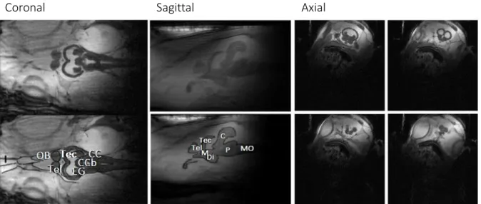
An anatomical drawing of T. japonicus is shown in figure 6 (Ou & Yamamoto 2016). Anatomical MR images of B. saida in a coronal, sagittal and axial plane are displayed in figure 7 with a description of different regions in the brain.
Figure 7: Brain regions of polar cod on MRI scans with OB, Tec, Tel, C, CC, eminentia granularis (EG), Corpus division of the Cerebellum (CCb), Mesencephalon (M), Diencephalon (Di), Pons (P) and Medula oblongata (MO)
Coronal Sagittal Axial
Figure 6: Technical drawing of the brain of B. saida with the olfactory tract (olt), olfactory bulb (OB), telencephalon (Tel), optic tectum (Tec), Cerebellum (C), cerebellar crest of the rhombencephalon (CC) and spinal cord (SC). Identification of the brain regions according to Ou & Yamamoto 2016 and Kawaguchi et al. 2019
o CC o
C o
Tel
Tec
SC OB
olt
10
Performing MR technology on marine animals is especially challenging (Van der Linden et al.
2004, Lee et al. 2010). Working with aquatic animals is challenging alone but seawater implies even more obstacles due to the high salt concentration. The animal inside the MRT needs a constant flow of aerated water (Van der Linden et al. 2004). But water motion can lead to artefacts in the MRI and it is crucial that the water does not come in contact with the gradient (Van der Linden et al. 2004). Therefore, different ways have been developed to overcome these obstacles. To guarantee a constant water flow without flooding the MRT, a metal free chamber can be used to place the fish inside the MRT, connected to water pools outside the MRT.
Different RF antenna have been evolved which can be placed in the water free space outside the chamber on top of the measured region (Van der Linden et al. 2004).
1.6 Chemical exchange saturation transfer
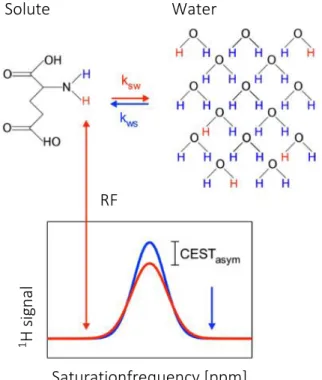
Recently, Ward et al. (2000) introduced a MRI technique that uses the exchange of protons (1H) as a contrast agent. This technique is called chemical exchange saturation transfer (CEST). Its principle is illustrated in figure 8. Exchangeable protons get excited by a set frequency and thereby selectively saturated which reduces magnetisation, ultimately leading to zero magnetisation. The saturated protons of the solute then exchange with the unsaturated protons in the tissue water with a defined exchange rate. The saturated protons accumulate in the tissue water leading to a reduced signal intensity of the water proportional to the solute concentration (Kogan et al.
2013). While the saturation frequency is applied and water magnetisation decreases, longitudinal relaxation brings the saturated protons back to their thermal equilibrium state (Kogan et al. 2013). The chemical shift between both resonance frequencies of the water and the solute protons is then measured in parts per million (ppm). The CEST effect is displayed in
Figure 8: The principle of CEST is illustrated above. Protons of a solute being saturated by a specific RF. Saturated protons of the solute then exchange with water protons, thereby decreasing the water signal proportional to the solute concentration. Modified illustration by Wermter (2017)
Solute Water
Saturationfrequency [ppm]
RF
1 H signal
11
the form of the z-spectrum (fig. 15) by plotting the water signal as a function of the saturation frequency and given in percent depending on the amount of exchanging protons (Kogan et al.
2013). The intensity of the CEST effect is pH and temperature dependant (Ward & Balaban 2000, Wermter et al. 2018)
CEST was tested with many different amino acids, such as alanine, glutamine or taurine as well as other solutes (Walker-Samuel et al. 2017). Taurine is important for neuronal activity and osmoregulation (Ripps & Shen 2012). Due to its osmoregulatory function, taurine is one of the most abundant amino acids in the brain of marine vertebrates and therefore easily detectable by the CEST application performed at low temperatures (Ripps & Shen 2012, Wermter et al.
2018). With the chemical exchange saturation transfer from taurine to water (TauCEST), it is possible to detect changes in the acid-base regulation of ectothermic animals, especially those living in a cold environment, like B. saida (Wermter et al. 2018). Wermter et al. (2018) were the first to investigate the TauCEST effect on the brain of the polar cod at high CO2 levels. The chemical shift between the amine protons of taurine and the water protons is assumed to be 2.8 ppm (Wermter et al. 2018). TauCEST is a non-invasive, in vivo method to detect even small changes in the pH under high CO2 exposure with high resolution (Wermter et al. 2018). By using
1H-NMR spectroscopy Wermter et al. (2018) could proof that the TauCEST in the brain of B. saida was not due to changes in the taurine concentration. In contrast to other in vivo methods this method gives the opportunity to see anatomical images of an unanaesthetised and ventilating fish, without the need for dissection (Wermter et al. 2018).
1.7 Hypotheses
The aim of this study will be to investigate pHi changes in the brain of B. saida caused by rising CO2 concentrations in the seawater. As previously mentioned, the polar cod is an important organism in Arctic waters as it links different trophic levels. Thus, it is of major interest to study its ecology and physiology in respect to a changing pHi as a result of OA.
Most studies that investigated the effects on pHi changes in the brain of marine animals so far have either been invasive, in vitro or they haven’t been conducted on polar fish species (Mark et al. 2002, Munday et al. 2011, Murray et al. 2014, Wermter et al. 2018). In order to investigate these changes, a combination of pHi determination with 31P-NMR spectroscopy and CEST will be applied and the following hypotheses are going to be tested:
12
• Hypercapnia induced acid-base regulation starts right after B. saida is exposed to environmental acidification and helps the cell to maintain pHi in hypercapnic conditions.
• B. saida is able to compensate the hypercapnia induced decrease in pHi over time
• pHi decreases during hypercapnia by up to 0.2 pH units
• The drop in pHe leads to metabolic depression in B. saida, effecting the cellular energy demand.
2 Material and Methods
2.1 Collection of the experimental animals
The animals used in this study were caught on the research vessel Heincke during the cruise HE 519 in October 2018. The animals were collected in a depth of 130 - 190 m, in a temperature of -1 - -1.5 °C in the Billefjord of Svalbard (78°59’N 16°50’E). The animals were captivated in a seawater aquarium at the Alfred-Wegener-Institute, Helmholtz Zentrum für Polar- und Meeresforschung (AWI) in Bremerhaven with a water temperature of 1 °C, a pH of 8 in normocapnia, a salinity of 32 PSU and were fed once a week.
2.2 Experimental setup
For each MR experiment, an individual fish was placed in a Perspex flow‐through chamber (V = 350 ml; fig. 9 A). Dental wax was added to the chamber and modulated for each fish individually positioning the fish at the frontal part of the chamber. All animals had enough space to move their fins and gills. Moreover, the seawater circulating system consisted of two heater tanks (ECO RE630, LAUDA GmbH & CO KG, Königshofen, Germany) which kept the water temperature in the chamber at around
0.5°C. Temperature confirmation measurements were performed inside the tanks with a high-precision temperature-measuring instrument (testo 112, testo, Lenzkirch, Germany) and at the outflow of the chamber with a fibre‐optical thermometer (OPTOCON
a
b
Figure 9: A: Testing chamber with the experimental animal inside and tubes with water inflow (a) and outflow (b). Dental wax helps to position the fish at the frontal part of the chamber. B: Schematic design of the experimental setup with the header tanks H1 (normocapnia) and H2 (hypercapnia), water inflow (A), water outflow (B) in an isolated tube (D), the experimental camber (E) and the MRT (F).
A
B
13
AG, Optical Sensors and Systems, Dresden, Germany). As displayed in figure 9 B each header tank was used for one sea water reservoirs (H1 and H2). H1 with control conditions bubbled with air; and H2 with elevated CO2 bubbled with an air/CO2 mixture from a gas‐mixing pump (PR 4000, MKS Instruments, Munich, Germany). The water reservoirs were changed once a week.
The pH of the water reservoirs was measured with a conventional pocket meter (pH 3310, WTW, Weilheim, Germany). Water pCO2 was determined from the gas phase of the sea water by a carbon dioxide sensor filter (CARBOCAP GMP343, Vaisala, Helsinki, Finland). Salinity was measured with a WTW LF 197 multimeter (WTW). Total alkalinity (TA) was measured in an external laboratory (Krisitina Beck, PhD Candidate, Bentho-Pelagic Processes, AWI, Bremerhaven). Since TA was measured only once, no standard deviation (SD) can be given.
Dissolved inorganic carbon (DIC) was measured via the continuous flow analysis method with Seal Analysis SFA QuAAtro (AACE 6.07, Seal Analytical, Wisconsin, USA). Bicarbonate (HCO3-)w was calculated via CO2Sys macro for Microsoft Excel (v2.1, Pierrot et al. 2006), with values for K1 and K2 from Millero (2010), KSO4 from Dickson (1990) and [B]T from Uppström (1974). A summary of water chemistry is given in Table 1. All tests were performed on a 9,4 T NMR- tomograph (BioSpec 94/30 USR, AVANCE III, Bruker BioSpin, Ettlingen, Germany). The in vivo
31P-NMR spectra were obtained by using a 2 cm diameter 1H/31P-NMR surface coil. The spectra were plotted and stacked with XWinPlot (Bruker BioSpin MRI GmbH, Ettlingen, Germany). The in vivo CEST measurements were performed on a 1H/13C resonator with an inner diameter of 72 mm.
All fish have been placed in the experimental chamber for at least 20 hours to acclimatise before switching to hypercapnia. Three hours prior to the hypercapnic treatment, control measurements were performed, followed by four hours of measurements under hypercapnia.
Afterwards, 2 more hours of normocapnia were recorded. The experimental protocol was the same for all in vivo MRI and NMR spectroscopy measurements.
All procedures were approved in accordance with the regulations for the welfare of experimental animals issued by the Federal Government of Germany (§11 Abs. Ziff. 1 a+b), Bremen AZ: 0515_2040_15.
14
Table 1:Seawater chemistry of the control (H1) and the hypercapnic (H2) water reservoirs. Temperature, salinity, pCO2, pHw, Total alkalinity and dissolved inorganic carbon were measured and HCO3- was calculated via CO2Sys macro for Microsoft excel (v2.1).
2.3 In vivo 31P-NMR spectroscopy
In vivo 31P-NMR spectroscopy was used to measure energy values and to determine the intracellular pH (pHi) in the brain of the fish (Lurman et al. 2007, Bock et al. 2008). The spectra were obtained by using a 2 cm diameter 1H-31P-NMR surface coil placed in the water free space outside the Perspex chamber above the head of the animal (fig. 10), to determine the chemical shift (δ) of the inorganic phosphate (Pi) signal relative to the Phosphocreatine (PCr) signal. δ was then used to calculate pHi by the following formula after Kost (1990) and modified after Bock et al. (2001).
𝑝𝐻𝑖 = 6.8788 + 𝐿𝑜𝑔10(𝑃𝑖 − 2.8) − 0.67 + 0.003579 ∗ 0.5 (3.2 + 0.001888 ∗ 0.5 − (𝑃𝑖 − 2.8)
PCr was used as an internal standard for spectra calibration and set to 0ppm. Furthermore, the intracellular energy values of tissue can be determined using 31P-NMR spectroscopy by calculating e.g. the ratio of Pi/PCr concentrations. The energy values were calculated as in the following formula.
𝐸𝑛𝑒𝑟𝑔𝑦 𝑣𝑎𝑙𝑢𝑒𝑠 = 𝐼𝑛𝑡𝑒𝑔𝑟𝑎𝑙 𝑜𝑓 𝑡ℎ𝑒 𝑃𝑖 𝑠𝑖𝑔𝑛𝑎𝑙 𝐼𝑛𝑡𝑒𝑔𝑟𝑎𝑙 𝑜𝑓 𝑡ℎ𝑒 𝑃𝐶𝑟 𝑠𝑖𝑔𝑛𝑎𝑙
Paravison 6.1 Software was used for all NMR measurements.31P-NMR spectroscopy scans were obtained with a flip angle of 65°, a repetition time TR = 1200 ms and 256 averages. Acquisition bandwidth was 10 000 Hz and reference power was 2.714 W. All scan properties are given in table 3 in the appendix.
Group T [°C] S [PSU] P (CO2)w
[ppm]
(HCO3-)w
[mM]
pHw TA
[mM]
DIC [mM]
Control 0.3 ± 0.2 30.5 ± 0.4 506 ± 24 1.96 7.96 ± 0.3 2.11 2.13 ± 0.06 Hypercapnia 0.7 ± 0.4 30.5 ± 0.5 3518 ± 110 2.15 6.92 ± 0.2 2.49 2.56 ± 0.1
15
2.4 CEST measurements
2.4.1 In vitro CEST measurements
Before the CEST in vivo experiments, a phantom study was performed to investigate the influence of the water parameters pH and temperature as well as the solute concentration of different metabolites found in the fish brain on the CEST effect. The in vitro measurements were based on a study by Wermter et al. (2018). The phantoms for the in vitro measurements consist of six NMR-tubes (Ø 5 mm) filled with different solutions bedded in a 50 ml Falcon Tube (Fisher Scientific GmbH, Schwerte, Germany) filled with a 3% Agarose solution. The agarose was mixed with deionized water and heated in a microwave until clear. After filling the agarose solution into the
Falcon tube, the NMR tubes were inserted (fig. 11). The solutions filled in the NMR-tubes are based on a phosphate buffer. The chemicals were obtained from Sigma Aldrich (St. Louis, USA). A summary of the in vitro phantom solutions is given in table 2. All solutions are adjusted to pH values of 6.5; 6.8;
7.0; 7.2, 7.5 and 7.8. All approaches were tested at seven different temperatures between 1 – 37°C.
In order to test the phantoms at different temperatures, a water hose (EHEIM GmbH & Co KG, Deizisau, Germany) was wrapped around the Falcon tube, isolated with isolating tape (ArmaFlex, armacell GmbH, Münster, Germany) and connected to a Thermostat (FP30 MH, JULABO GmbH, Seelbach, Germany). The phantom tubes were attached to a positioning aid to push them into the magnet. The object to be tested has to be in the centre of the magnet to get the best possible image.
CEST images were obtained by pre-saturated FISP (fast imaging with steady state precession) scans with a field of view (FOV) 30 x 30 mm2, a matrix size of 64 x 64, a slice thickness of 2 mm, a flip angle of 9°, a repetition time TR = 3.2 ms and an echo time TE = 1.6 ms. Before measuring the CEST effect, B0 Figure 10: in vivo MR image of the head of B. saida
obtained with a 1H/13C resonator with an inner diameter of 72 mm. The yellow circle marks the area sensitive to the 31P-NMR-surface coil.
Figure 11: Phantom tube with different pH values of the same solution in the NMR tubes for the in vitro CEST study.
16
homogeneity was optimized to a line width of 10 Hz or less. Z‐spectra were obtained using 50 frequency offsets between −20 000 and 20 000 Hz with respect to the water signal. The experimental design for the in vitro study is shown in figure 12. All scan properties are given in table 3 in the appendix.
Table 2: Three different approaches for the in vitro CEST measurement. One negative control only consisting of PBS. One solution with PBS and BSA [10 mM] and one solution with PBS and TMAO [10mM]. Chemicals with the used concentrations to produce PBS are listed below. All solutions were adjusted to the following pH values: 6.5; 6.8; 7.0; 7.2, 7.5 and 7.8 and tested at seven different temperatures.
Approach Solute Concentration
[mM]
Temperature [C°]
Negative control - Phosphate buffered saline (PBS)
NaCl 137.0 1, 5, 10, 15,
20, 25, 37
KCl 2.7
Na2HPO4 * 2H2O 10.0
KH2PO4 1.8
PBS + Bovine serum albumin (BSA)
PBS
BSA 10
1, 5, 10, 15, 20, 25, 37 PBS + Trimethylamine N-oxide
(TMAO)
PBS
TMAO 10
1, 5, 10, 15, 20, 25, 37
All scan images with different excitation frequencies were stacked to a hyperstack. In every hyperstack the different regions of interest (ROI) in the NMR tubes were selected (fig. 13) and evaluated in Fiji image J (Schindelin et al. 2012, Rueden et al. 2017). The data gained from Fiji
Figure 12: Experimental design of the in vitro study with A: header tank; B: water hose; C:
isolation; D: NMR tubes with the testing solution;
E: magnet resonance tomograph. On the left the realistic proportions are shown.
17
image J was loaded into MATLAB (Version R2019a, The MathWorks Inc., Natick, USA). Z-Spectra (exepmlary shown in fig. 14) were generated in MATLAB.
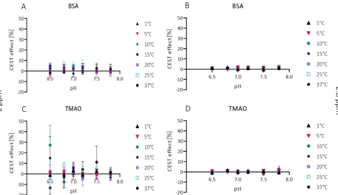
The CEST effect for a chemical shift at 1 ppm and 2.8 ppm were evaluated (fig. 15). TMAO shows a mean CEST effect for a pH value of 6.5 of
15% ± 20% (15°C) and 27% ± 19% (10°C) as well as a CEST effect of 11% ± 15% for a pH value of 7.5 at 37°C and a chemical shift of 1 ppm. BSA does not show any CEST effect higher than 6% ± 4%, also at a chemical shift of 1 ppm. The CEST effect is much higher for a chemical shift of 1 ppm than for a chemical shift of 2.8 ppm. A graph with a smaller scale for a chemical shift of 2.8 ppm is shown in the appendix
1 2 3
4 5 6
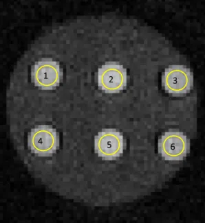
Figure 13:MR image of a phantom with a different pH value (6.5; 6.8; 7.0; 7.2; 7.5; 7.8) in each tube. The yellow circles show the chosen ROI that was evaluated first in Fiji image J and then in MATLAB.
Figure 14: Z-spectra showing the CEST effect in percent for a chemical shift of 1 ppm and 2.8 ppm. In A with a high CEST effect and in B no CEST effect. A shows the CEST effect for TMAO at 15 °C at a pH of 7. B shows the CEST effect for BSA at 5°C at a pH of 7.5.
A B
18 2.4.2 In vivo CEST measurements
Pilot and RARE scans (Rapid acquisition with relaxation enhancement) were conducted before the in vivo CEST measurements, were performed to detect an optimal slice of the brain. A MRI slice which displays a preferably large area of the brain was chosen for CEST.
Measurements were performed in triplets alternating with RARE scans to control the position of the fish. The chosen slice with the ROI is shown in figure 16.
Figure 16: Testing slice for the in vivo CEST measurements with the chosen ROI in the yellow box. The MRI scan was obtained with a 1H/13C resonator with an inner diameter of 72 mm.
Figure 15: The CEST effect for a chemical shift of 1 ppm in A (BSA) and C (TMAO) and for a chemical shift of 2.8 ppm in B (BSA) and D (TMAO). TMAO shows a CEST effect for δ 1ppm at a pH of 6.5 and a temperature of 10°C and 15°C.
A B
C D
2.8 ppm
1 ppm [%] [%] [%] [%]
19 2.5 Statistical analysis
For any significance analysis ANOVA with post-hoc tests were performed in GraphPad Prism (Prism Version 8.1.2., GraphPad Software, Inc., San Diego, USA). All graphs were plotted in GraphPad Prism. ANOVA tests were conducted with the pHi values of three hours before switching to hypercapnia. The pHi values under hypercapnia as well as the pHi values under normocapnia were evaluated against the mean of the pHi values under control conditions.
3 Results
3.1 In vivo 31P-NMR spectroscopy
With in vivo 31P-NMR spectroscopy it is possible to visualise the abundance and the concentration of phosphometabolites such as sugar phosphates (sP), cyclic adenosinmonophosphate (cAMP), inorganic phosphate (Pi), phosphodiester (Pd), phosphocreatine (PCr) and three different adenosinetriphophate (ATP) subunits α-, β- and γ γ,Figure 17 presents such a spectrum obtained by in vivo 31P-NMR spectroscopy under control conditions. All the phosphometabolites mentioned above could be detected. Figure 18 displays the effect of different pH values on the position of Pi and its chemical shift δ to PCr.
PCr
ATP Pi Pd
sP cAMP
Figure 17: Typical in vivo 31P-NMR spectrum showing relative concentrations of phosphometabolites in a brain cell of B. saida. Phosphometabolites in the brain are sP = sugar Phosphates; cAMP = cyclic AMP; Pi = inorganic Phosphate; PCr = Phosphor creatine and the three phosphate groups γ-, α- and β-ATP. The PCr peak was set to 0 ppm. The other metabolites have a chemical shift in ppm in relation to PCr.
δ
γ α β
20
Figure 19 A shows a stack plot of in vivo 31P-NMR spectra two hours of control conditions prior to hypercapnic conditions. The signal intensity of the ATP signals is relatively stable before switching to hypercapnia, while the PCr and Pi signals show some fluctuations. The first two hours under hypercapnic conditions are displayed in figure 19 B. The signal intensity of PCr is diminished after switching to hypercapnia but increases again over time. The acquisition of each spectrum takes five minutes. As shown in figure 19 C the PCr signal intensity decreases after switching back to normocapnia but also increases again after one hour. All stacked spectra are exemplarily shown for fish 3.
Figure 18: Two 31P-NMR spectra showing a different chemical shift of Pi in relation to PCr. The difference in δ between the two displayed spectra is 0.11 ppm.
δ
21 A
B
C
Figure 19: Stacked 31P-NMR spectra of A: two hours of control conditions before switching to hypercapnia. B: the first two hours of hypercapnic conditions and C: the recovery time under normocapnic conditions after hypercapnia. The stacked spectra show the fluctuations in the signal intensity of the phosphometabolites. The acquisition of every spectrum takes five minutes. The displayed spectra were acquired in experiments with Fish 3.
22 3.2 Energy values
Fish 1 was showing a much higher Pi/PCr ratio during the whole experiment than the other three fish (fig. 20 A). The values for fish 1 in hypercapnic conditions are significantly higher than the values in control conditions. This is not the case for any of the other three fish (fig. 20 B-D).
The Pi/PCr ratio of all four fish is displayed in figure 20 A-D. The energy values stay relatively stable during the complete time of the experiment for fish 2, 3 and 4 (fig. 20 B-D). The values of Pi/PCr ratio are in an expected range (0.05 - 0.6 ru) when compared to Kushmerick et al.
(1992), Burgard (2004) and Bock et al. (2019). A relation of the Pi/PCr ratio of all four fish is shown in figure 20 E.
Figure 20:The energy values of every fish indicated by the Pi/PCr ratio, given in relative units [ru], and displayed in A-D. A comparison of all fish is shown in E. Time 0 is 3 hours before switching to hypercapnia.
A B
C D
E
23 3.3 pHi regulation
Diagrams for all fish start with a three hour control before switching to hypercapnia, then four hours of hypercapnic conditions and then two hours of normocapnic conditions, except for fish 1 where only one hour of normocapnia could be performed. Every datapoint is 15 minutes apart from the following and represents the mean value of three 31P-NMR spectroscopy measurements.
3.3.1 Fish 1
The mean pHi of fish 1 during control is 7.46 ± 0.08 and decreases during hypercapnia by 0.6 pH units to a minimum of 6.87 ± 0.02. The mean pHi during hypercapnia is 7.18 ± 0.08. After the hypercapnic treatment fish 1 shows an overshooting pHi of the mean normocapnic value of 0.13 pH units to a pHi of 7.59 ± 0.24 compared to the mean control and a maximum overshoot of 0.3 pH units (fig. 21). The pHi as well as the pHw were much lower for fish 1 compared to fish 2, 3 and 4. Nevertheless fish 1 survived and was still alive five weeks after the experiment. However, the energy values as well as the pHi and pHw of fish 1 indicate an altered experimental setup which is why fish 1 will not be taken into account for further statistical tests and will be discussed on its own. All figures showing mean values of all fish, show mean values of fish 2;3 and 4. Stacked spectra of fish 1 can be seen in the appendix (fig. 32-35).
Figure 21: pHi and pHw of fish 1 during the experiment. Since pHw was especially low on this experiment day it is plotted separately (red line).
Control Hypercapnia Norm.