Boreogadus saida , to environmental hypoxia: critical oxygen level and swimming performance The physiological response of an Arctic key species Polar cod,

(1)

The physiological response of an Arctic key species Polar cod, Boreogadus saida, to environmental

hypoxia: critical oxygen level and swimming performance

Sarah Kempf Master Thesis University of Bremen

First Supervisor: Dr. Felix Christopher Mark (AWI) Second Supervisor: Dr. Andreas Kunzmann (ZMT)

Edited Version: February 18^th 2020

(2)

List of Figures and Tables

Figures

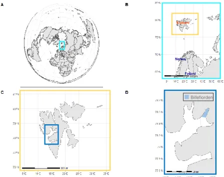
Figure 1 Study area Billefjorden (Svalbard archipelago). A: position of the Svalbard archipelago on a world map. B: position of the Svalbard archipelago in context of mainland. C: enlarged map of the Svalbard archipelago. D: exact position of Billefjorden. ... 3 Figure 2 Comparison Kongsfjorden and Billefjorden. Upper row: depth profile of Kongsfjorden (04.10.2018) (11.6928°E, 78.9840°N), Lower row: depth profile of Billefjorden (06.10.2018) (16.4997°E, 78.5883°N), plots from left to right: temperature (°C), salinity (psu) and oxygen saturation (%) with increasing depth. (Data from: Mark and Wisotzki 2018). ... 4 Figure 3 Projected changes from 1961–90 to 2071–2100 in mean annual temperature (°C) The RCM projections are based on MPIB2 (for acronyms, see Appendix Table 12; for weather stations used in the analysis, see Appendix Figure 21) (Førland, Benestad et al. 2011). ... 5 Figure 4 Temperature projections for Svalbard Airport/Longyearbyen: results from ESD and RCM downscalings for winter, spring, summer, and autumn. The hatched area (pink) shows 5 % and 95 % interval from ESD estimates, the black dots show observed values, and the thick line (red) show median (50 %) value for the ESD ensemble. The coloured symbols indicate the median value for the different runs with NorACIA-RCM, and the vertical lines show the 5- and 95- percentiles for the RCM runs. The RCM values are plotted on the central year in the respective time slices. (for acronyms, see Appendix Table 12; for weather stations used in the analysis, see Appendix Figure 21) (Førland, Benestad et al. 2011). ... 6 Figure 5 Hydrographic profile along the main axis of Billefjorden (August 2001) A: salinity, B:

Water masses are marked by a dotted line, the shaded area marks land masses; SW – surface water, IW – intermediate water, LW – local water, WCW – winter-cooled water (modified after Szczuciński, Zajączkowski et al. 2009). ... 7 Figure 6 Limiting oxygen level (LOL) curve. The ambient oxygen saturation [%] influences the aerobic metabolic capacity of an idealized organism (modified after Claireaux and Chabot 2016).

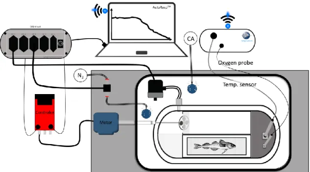
Shown are the maximum sustainable metabolic rate (MMR) (red dashed line) and standard metabolic rate (SMR) (green dashed line), the LOL curve (black), aerobic scope (distance between LOL curve and SMR) and the critical oxygen level (Pcrit) (Neill and Bryan 1991, Claireaux and Chabot 2016). ... 9 Figure 7 Schematic construction of the respirometry system. All respiration chambers are connected to one recirculation pump and one flush pump. Within the recirculating water, flow probe vessels are included where the oxygen probes are located. A four-channel oxygen meter (Loligo systems ApS, Denmark, Witrox 4 oxygen meter for mini sensors) detects the ambient oxygen in the chambers and basin as well as temperature, sending the data via Bluetooth to a

(5)

ii

computer with the software AutoResp version 2.3.0 (Loligo Systems ApS, Denmark). Compressed air (CA) together with nitrogen (N2) create the desired oxygen concentration (100 - 5 % saturation).

The data acquisition instrument (DAQ-M) controls the flush and recirculation pumps and the amount of nitrogen pumped into the water. DAQ-M is also connected to and controlled by a computer with the software AutoResp. ... 12 Figure 8 Schematic construction of the swim tunnel A four-channel oxygen meter (Loligo systems ApS, Denmark, Witrox 4 oxygen meter for mini sensors) detects the ambient oxygen in the swim tunnel as well as temperature, sending the data via Bluetooth to a computer with the software AutoResp version 2.2.0 (Loligo Systems ApS, Denmark). Compressed air (CA) together with nitrogen (N2) create the desired oxygen concentration (100 – 10 % oxygen saturation). The data acquisition instrument (DAQ-M) controls the flush pump and the amount of nitrogen pumped into the water. DAQ-M is also connected to and controlled by a computer with the software AutoResp.

A motor regulated by the controller drives the propeller, creating a laminar current within the swim tunnel. The fish is placed in the operation part of the tunnel. ... 14 Figure 9 Standard metabolic rate (SMR). Shown are the metabolic rates ((MR) in µmol O2/g∙h) (orange circles) recorded at 56 - 100 % PO2. The SMR (0.44µmol O2/g∙h; black line) was calculated as described under point 2.4.3 using the R package “Mclust” after Chabot et al. (2016). ... 19 Figure 10 Routine metabolic rate (RMR). Shown are the metabolic rates ((MR) in µmol O2/g∙h) (orange circles) (86 experimental runs representing 1887 single metabolic rate data points of 30 individuals) performed between 5 and 100 % PO2 in respiration chambers. The RMR (dark orange line, with SD (light orange area)) was calculated as described under point 2.4.4. Black line: standard metabolic rate (SMR; 0.44 µmol O2/g∙h). ... 20 Figure 11 Maximum metabolic rate (MMR). Shown are the metabolic rates ((MR) in µmol

O2/g∙h) (blue circles) (60 experimental runs representing 361 single metabolic rate data points of 30 individuals) performed between 10 and 100 % PO2 in the swim tunnel. The MMR (dark blue line, with SD (light blue area)) was calculated as described under point 2.4.5. Black line: standard metabolic rate (SMR; 0.44 µmol O2/g∙h). ... 22 Figure 12 Routine- (RMR), maximum- (MMR) and standard metabolic rate (SMR) of 148

single measurements with a total of 30 multiple used individuals. Metabolic rates ((MR) in µmol O2/g∙h) at the different oxygen saturation (%). Data from both, swim tunnel and respiration chamber, experiments. In blue: metabolic rate of 60 individuals recorded during swim tunnel experiments. In orange: metabolic rate of 86 individuals recorded during measurements in respirometry chambers. Upper blue line: maximum metabolic rate (swimming tunnel; calculated as described in 2.4.5). Lower dark orange line: routine metabolic rate (respiration chambers;

calculated as described in 2.4.4). Black line: SMR (respiration chambers; calculated as described in 2.4.3). Grey shaded area: aerobic scope (difference between MMR and RMR)... 24

(6)

iii

Figure 13 Aerobic scope. Bars represent the mean aerobic scope of Polar cod at ten different oxygen saturations (treatments). The different grey shadings represent three significantly different levels of AS. Aerobic scope was calculated as described in 2.4.6. Error bars depict standard deviation. Asterisks: significant difference between the three decreasing levels of AS (***, or a, b, c for the three steps), all p-values are lower than 0.0001. ... 24 Figure 14 Limiting oxygen level (LOL) curve after Claireaux and Chabot (2016). Shown are the maximum metabolic rate (MMR; blue line) and standard metabolic rate (SMR; black line), MMR regression line (dashed blue line; polynominal regression of the MMR between 10.77 and 25.36 % PO2 (y= 1E-06x² + 0.0002x – 0.0005; R²= 0.9994)), the critical oxygen level (Pcrit (4.81

%), red circle, intersection between MMR regression line and SMR) and the scope of survival (between 1.71 and 4.81 % PO2). ... 25 Figure 15 Metabolic rates over increasing water velocities. Boxplots (with median and outliers) show the results of the swim tunnel measurements. Displayed are the MR [mmol O2/g∙h] during increasing water velocities [BL/sec]. Letters indicate results of Tukey honest significance test between Velocity treatments. Significant differences are represented by different letters, the corresponding p-values can be found in Table 3.(n per velocity: 1.40=59, 1.55=59, 1.70=60, 1.85=56, 2.00=45, 2.15=38, 2.30=21, 2.45=12, 2.60=8 ,2.75=2 ,2.90=1). ... 26 Figure 16 Gait transition speed (Ugait) over increasing oxygen concentrations. Comparison of Ugait

(BL/sec) at different oxygen levels (n per treatment: 10=1, 15=2, 20=3, 25=6, 30=6, 40=5, 50=6, 60=6, 70=6, 100=6). No significance between PO2 treatments was observed. ... 28 Figure 17 Critical swimming speed (Ucrit) over increasing oxygen concentrations. Comparison of Ucrit (BL/sec) at different oxygen levels (n:6 per treatment). Letters indicate results of Tukey honest significance test between PO2 treatments (p= 0.031). All other p-values can be found in Table 6. 29

Figure 18 Turbine calibration. The turbine rotation was calibrated using a flowmeter. Turbine rotation was increased in steps of 10 rpm, de corresponding water velocity in m/s were detected with a flowmeter. Water velocity was measured at the bottom of the working section in the swim tunnel. This was repeated randomly for the middle and top layer of the working section. Linear regressions though the values measured in the middle and top region to calculate the corresponding water velocity at 1020 rpm. This calibration data was used to determine the actual water velocity within the swim tunnel. ... xxiii Figure 19 Pcrit calculation. Shown are SMR (black), RMR (orange), MMR (blue), RMR linear regression line (dotted orange) and MMR polynomial regression line (dotted blue). ... xxiii Figure 20 Pcrit of marine species grouped by temperature range -1.5 to 20°C. Values represent the respective mean Pcrit (± SE). Numbers contained within each bar indicate the temperature (°C) at which Pcrit was determined. Blue shaded bars mark data of Polar- or Gadidae species, relevant

(7)

iv

for this study. Yellow bar: Pcrit of B. saida determined in this study and included in this database (modified after Rogers et al. 2016). ... xxxii Figure 21 Map of the Svalbard region including weather stations used in the analysis (Førland, Benestad et al. 2011). ... xxxiii Figure 22 Annual temperature development at weather stations in the Svalbard region. The lowpass filtered series are smoothed by Gaussian weighting coefficients and show variability on a decadal time scale. The curves are cut three years from start and end (Førland, Benestad et al.

2011). xxxiv

Figure 23 Collection of metabolic scopes of European sea bass (Dicentrarchus labrax), Atlantic cod (Gadus morhua), common sole (Solea solea) and turbot (Psetta maxima) as a function of ambient dissolved oxygen. MS is shown on absolute scale (a) and relative to normoxia (b) (Chabot and Claireaux 2008). ... xxxiv

(8)

v Tables

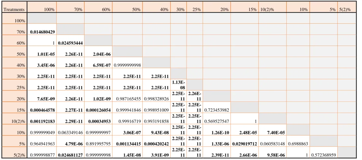
Table 1 P-values of TukeyHSD, RMR. Comparison of all treatments and the corresponding metabolic rates from respirtometry chambers. Significant p-values are printed in bold type.

Treatments 10 and 5% PO2 have been repeated due to recalibration of the oxygen optodes. ... 21 Table 2 P-values of TukeyHSD, MMR and PO2. Comparison of all treatments and the corresponding metabolic rates from swim tunnel. Significant p-values are printed in bold type. 23 Table 3 P-values of TukeyHSD, MMR and velocity. Comparison of all velocity treatments and the corresponding metabolic rates from swim tunnel. Significant p-values are printed in bold type.

27

Table 4 Burst activity. Mean total number of bursts (with standard deviation, SD) and mean bursts per minute (with SD) of all fish ordered by PO2 treatments. ... 28 Table 5 Swimming activity. Mean percentage of active (with standard deviation, SD) and inactive phases (with SD) and the mean of the total swim time [min] (with SD) during the swim tunnel experiments ordered by PO2 treatments. ... 30 Table 6 P-values of TukeyHSD, Ucrit and PO2. Comparison of all treatments and the corresponding metabolic rates from swim tunnel. Significant p-values are printed in bold type. 30 Table 7 Fish-tagging. Serial number of the implanted passive glass transponder (PIT), the fish weight [g], total- and standard length [cm], width [cm] (vertical axis, measured at the thickest point) and depth [cm] (horizontal axis, measured at the thickest point). ... xxii Table 8 Ugait [rpm and BL/sec] and Ucrit [rpm and BL/sec] for all fish ordered by the different PO2 treatments. ... xxiv Table 9 Raw data bursts. Ordered by PO2 Treatments, TSB = time spent bursting. ... xxvi Table 10 Raw data swimming time. Ordered by PO2 Treatments, TMT = total measurement time, sec. inactive = inactive period per fish in seconds during measurement time. ... xxix Table 11 Average annual and seasonal temperatures (◦C) during 1961–90 and 1981–2010 (Førland, Benestad et al. 2011). ... xxxiii Table 12 RCM simulations for the Svalbard region. The simulations were performed by the regional climate model HIRHAM2/NorACIA (Førland, Flatøy et al. 2009, Førland, Benestad et al.

2011). xxxiv

(9)

vi

List of Abbreviations

α O2 solubility coefficient after Boutilier et al. 1984

µmol micromole

ANOVA analysis of variance

AS aerobic scope

AWI Alfred-Wegener-Institute Helmholtz Center for Polar and Marine Research B. saida Boreogadus saida, Polar cod

BL body length

BW body weight

CO2 carbon dioxide

EPOC post-exercise oxygen consumption HPLC high performance liquid chromatography IPCC Intergovernmental Panel on Climate Change IW intermediate water

LOL limiting oxygen level

LW local water

mmol millimole

MMR maximum metabolic rate

MO2 oxygen consumption

O2 molecular oxygen

OCLTT oxygen & capacity limited thermal tolerance PCO2 carbon dioxide partial pressure

PO2 oxygen partial pressure

∆PO2 change in water PO2 [kPa]

pMMR p-values for the swim tunnel experiment

PRMR p-values for the respirometry chamber experiment RMR routine metabolic rate

rpm rotations per minute SMR standard metabolic rate

SW surface water

t time interval

∆t elapsed time

T time spent at the given velocity leading to exhaustion of the fish

(10)

vii Temp. temperature

Ucrit critical swimming speed (maximum achievable swimming speed)

Ugait gait transition speed (transition phase of purely aerobic and partly anaerobic swimming)

Umax highest velocity (v) perpetuated for a complete time interval (t)

v velocity

V volume

WCW winter cooled water

(11)

viii

Summary

Since the beginning of the industrialization, uncontrolled greenhouse gas emission led to a distinct temperature increase on earth. Arctic environments are projected to experience the most severe changes due to climate change. Higher atmospheric temperatures caused already various environmental changes, for example a decrease in Arctic sea ice of 49 % (1979-2000) and increasing carbon dioxide concentrations which reduced the sea surface pH. A reduced sea ice formation will strengthen the summer stratification of warm, oxygen poor on top of cold, oxygen rich water masses, which may consequently cause local hypoxia in ground water layers.

As a result, the deep cold water layers do not receive oxygen-rich water and oxygen consumption extends over more than one season. This can lead to local hypoxia in the ground water layers of the protected fjords. Especially endangered of this long-lasting stratification in winter are the deep fjord systems of the Svalbard archipelago. In this region, the change of winter temperatures from 1961–90 corresponded to an increase of 0.6 °C per decade.

Corresponding, an additional increase of 0.9 °C per decade is projected for 2071–2100. Thus, the present study investigates the hypoxia tolerance of Polar cod, Boreogadus saida, one of the main Arctic key species. Therefore, different performance parameters were determined. The respiratory capacity as well as the swimming performance under declining oxygen concentrations were measured in two different experimental setups. A sample size of 30 Polar cod with similar body length and weight were chosen. All individuals were used several times during the experiments. First, the routine (RMR) and standard metabolic rate (SMR) were determined via flow-through respirometry. The calculated SMR for Polar cod accounted 0.44 µmol O2/g∙h. The RMR followed an oxygen regulating pattern, indicating that aerobic metabolic pathways such as lipid oxidation were used, rather than anaerobic pathways. This implies a relatively small contribution of anaerobic metabolism to the energy production in B.

saida. This was confirmed in the swim tunnel experiments. However, Ugait (the speed at which the fish changed to anaerobically fuelled swimming) was not significantly affected by hypoxia, the total number of bursts (p = 0.025) and total active swimming time (p = 0.017) significantly decreased with decreasing oxygen saturation. The loss of anaerobic swimming capacity due to hypoxia may endanger this species in regard to predator-prey-interactions and loss of escape reactions. Under exercise Polar cod was able to up-regulate its maximum metabolic rate (MMR) until a threshold of 45 % PO2 was reached. Afterwards, the oxygen consumption significantly decreased with decreasing oxygen concentrations. Throughout both experiments neither RMR nor MMR decreased below SMR level. Furthermore, the present study revealed that Polar cod

(12)

ix

is an extremely hypoxia tolerant fish species, which is able to handle oxygen saturations down to a Pcrit of 4.81 % PO2. This outstanding capability could give the otherwise rather disadvantaged fish species an advantage under changing climate conditions.

(13)

x

Zusammenfassung

Seit Beginn der Industrialisierung führte der unkontrollierte Ausstoß von Treibhausgasen zu einem deutlichen Temperaturanstieg auf der Erde. Für die Arktis werden die stärksten Veränderungen durch den Klimawandel prognostiziert. Höhere atmosphärische Temperaturen verursachten bereits verschiedenste Umweltveränderungen, wie zum Beispiel eine Abnahme des arktischen Meereises um 49 % (1979-2000) und steigende Kohlendioxidkonzentrationen, die den pH-Wert der Meeresoberfläche stark senkten. Eine verringerte Meereisbildung wird die sommerliche Schichtung von warmen, sauerstoffarmen und kalten, sauerstoffreichen Wassermassen verstärken, was zu einer lokalen Hypoxie in den Grundwasserschichten führen kann. Besonders gefährdet von dieser langanhaltenden Trennung der Wassermassen im Winter sind die tiefen Fjordsysteme des Svalbard-Archipels. In dieser Region entsprachen Temperaturveränderungen zwischen den Jahren 1961 und 1990 einem Anstieg um 0,6 °C pro Jahrzehnt. Anhand dieser Veränderung wird für den Zeitraum von 2071 bis 2100 ein weiterer Anstieg um 0,9 °C pro Jahrzehnt prognostiziert. Die vorliegende Studie untersucht daher die Hypoxie-Toleranz von Polardorsch, Boreogadus saida, einer der wichtigsten arktischen Schlüsselarten. Dazu wurden verschiedene Leistungsparameter ermittelt. Sowohl die Atmungskapazität als auch die Schwimmleistung bei abnehmenden Sauerstoffkonzentrationen wurden in zwei verschiedenen Versuchsaufbauten gemessen. Es wurde eine Probengröße von 30 Polardorschen mit ähnlicher Körperlänge und ähnlichem Gewicht gewählt. Alle Individuen wurden während der Experimente mehrfach verwendet. Zunächst wurden die Routine- und die Standard-Stoffwechselraten mittels Durchflussrespirometrie bestimmt. Der berechnete Standard-Stoffwechsel für den Polardorsch betrug 0,44 µmol O2/g∙h. Der Routine-Stoffwechsel folgte einem sauerstoffregulierenden Muster, was darauf hinweist, dass aerobe Stoffwechselwege wie die Lipidoxidation genutzt wurden und anaerobe Stoffwechselwege für diese Arte eine kleinere Rolle spielen. Dies impliziert einen relativ geringen Beitrag des anaeroben Stoffwechsels zur Energieproduktion in B. saida. Dies wurde in den Schwimmtunnel-Experimenten bestätigt. Auch wenn Ugait (die Geschwindigkeit bei, der die Fische zu anaerob angetriebenem Schwimmen übergingen) nicht signifikant durch Hypoxie beeinflusst wurde, konnte ein signifikanter Zusammenhang zwischen einer sinkenden Gesamtzahl der Bursts (p = 0,025) sowie einer Abnahme der gesamten, aktiven Schwimmzeit (p = 0,017) mit abnehmender Sauerstoffsättigung gezeigt werden. Dieser Verlust der anaeroben Schwimmkapazität durch die Hypoxie kann diese Spezies in Bezug auf Raubtier-Beute- Interaktionen und den Verlust von Fluchtreaktionen unter zukünftigen Umweltbedingungen

(14)

xi

stark gefährden. Unter Belastung konnte der Polardorsch seine maximale Stoffwechselrate hochregulieren, bis ein Schwellenwert von 45 % PO2 erreicht wurde, danach nahm der Sauerstoffverbrauch mit abnehmender Sauerstoffkonzentration im Wasser signifikant ab.

Während beider Experimente sanken die Stoffwechselraten nie unter das Niveau des Standard- Stoffwechsels. Darüber hinaus zeigte die vorliegende Studie, dass Polardorsch eine extrem hypoxietolerante Fischart ist, die mit Sauerstoffsättigungen bis zu einem Pcrit von 4,81 % PO2

umgehen kann. Diese hervorragende Fähigkeit könnte dieser sonst eher benachteiligten Fischart unter veränderten Klimabedingungen einen Vorteil verschaffen.

(15)

1

Introduction

Since the polar oceans are expected to warm twice as fast as the global average, polar key species such as Boreogadus saida are ideal model organisms to understand physiological responses to global warming and predicted future ecosystem scenarios (Hoegh-Guldberg and Bruno 2010, Hop and Gjøsæter 2013, Fossheim, Primicerio et al. 2015). Changes in abundance of B. saida, either caused directly by ecological changes driven by global warming or indirectly by invasion of predators and competition among immigrating species, have grievous consequences on the whole ecological system (Craig, Griffiths et al. 1982, Welch, Bergmann et al. 1992, Orlova, Dolgov et al. 2009). Therefore, it is of great interest to determine the ecophysiological thresholds of this key species for the changing parameters in future climate scenarios. Based on the unknown physiological response of Polar cod to progressive hypoxia, three major questions arose. (1) Does progressive hypoxia influence its metabolic rate? (2) Does the swimming performance of Polar cod respond to diminishing oxygen availability? (3) In which oxygen range do we find the critical oxygen concentration (Pcrit) concentration of Polar cod? To answer those questions, oxygen uptake and swimming performance were recoded as physiological performance parameters under progressive hypoxia. Concerning the swimming performance, I hypothesise that the critical swimming speed (Ucrit) should be reached earlier with progressing hypoxia. Earlier studies showed that scant oxygen availability lowers the maximum metabolic rate (MMR) and therefore decreases the energy supply (Pörtner 2010).

Compared with previous studies where polar cod was exposed to hypercapnia together with increased temperature, high sensitivities of maximum performance parameters (MMR, Ugait, Ucrit) were revealed (Kunz, Claireaux et al. 2018). Comparing to other Gadidae species, Atlantic cod (Gadus morhua) reduced swimming speed by 21 – 41 % under hypoxia (20 – 40 % oxygen saturation) (Herbert and Steffensen 2005). Furthermore, based on studies on other Gadidae species as Atlantic cod (Gadus morhua) and Greenland cod (Gadus ogac) the Pcrit of Polar cod can be assumed to be found between 25 and 40 % oxygen saturation (Steffensen, Bushnell et al. 1994, Rogers, Urbina et al. 2016) (Appendix Figure 20).

(16)

2 1.1 Study animal

The Polar cod (Boreogadus saida (Lepechin, 1774)) belongs to the family of Gadidae and is a generally small fish with an average maximum length of 30 cm (Scott and Scott 1988, Hop and Gjøsæter 2013). It reaches an average age of seven years (Hop, Welch et al. 1997). Males become mature at an age of two, whereas females first mature later, on average at an age of three years (Craig, Griffiths et al. 1982). Spawning takes place between December and March, peaking in January and February at a preferred spawning temperature of 1 – 2 °C (Hognestad 1966, Hognestad 1968). B. saida has a circumpolar distribution in waters with and without drifting sea ice (Ponomarenko 1968, Cohen, Inada et al. 1990). They feed on invertebrate species (Gastropoda, Larvacea, Chaetognatha), but mainly on Crustaceans like copepods (Calanus finmarchicus, Calanus glacialis) (Lønne and Gulliksen 1989). Polar cod itself is an important prey for various animals, such as birds, whales, and fish, including economically important fish species (Bradstreet 1982, Welch, Crawford et al. 1993). The core thermal habitat of B. saida is dependent on the life stage of the fish. The main thermal habitat of juveniles (0- group index) is 2.0 - 5.5 °C (Eriksen, Ingvaldsen et al. 2015), whereas adult fish (>age-1 fish) caught in the Canadian Beaufort Sea are found in regions of >0 °C between 20 and 1000 m depths (Majewski, Walkusz et al. 2016). Other studies showed that adult Polar cod inhabits the upper 20 m with temperatures above -1.5 °C and up to >2 °C as well as deeper waters (~130 m) with temperatures of -1.3 to -0.3 °C (Crawford and Jorgenson 1996, Crawford, Vagle et al.

2012). Although it was found that B. saida can cope short-term with temperatures up to 15.2

°C until cardiac arrhythmia sets in, the mean upper thermal limit that triggered cardiac arrhythmia is 12.4 °C, tested in a field study in Nunavut (Drost, Carmack et al. 2014). Drost et al. (2014) as well as other studies on both the cardiac mitochondrial function in response to environmental hypercapnia (Leo, Kunz et al. 2017) and the swimming behaviour under elevated temperatures (Schurmann and Christiansen 1994) showed that long-term exposure to increased temperatures decrease the fitness of Polar cod way before 12°C. Leo et al. (2017) showed that temperatures above 8 °C led to a decreased mitochondrial efficiency. Further experiments on the metabolism and performance of polar cod under ocean acidification and warming proved that the optimum growth performance under normocapnia was achieved at 6 °C, whereas the highest feed conversion efficiency was performed at 0 °C. Hypercapnia resulted in small losses in growth performance, but no significant temperature effect was observed (Kunz, Frickenhaus et al. 2016). In the study of Schurmann and Christiansen (1994), the preferred temperature for swimming activity was determined between 2.8 - 4.4 °C. This indicates that Polar cod has a confined ability to acclimate to rising temperatures.

(17)

3 1.2 Study area under climate change

Fjords on the west coast of Spitsbergen are influenced by hydrographically different water masses such as Atlantic-, Arctic-, brine-, and freshwater inputs. As they balance these diverse hydrographic influences, they are sensitive indicators for environmental changes (Nilsen, Cottier et al. 2008).

Figure 1 Study area Billefjorden (Svalbard archipelago). A: position of the Svalbard archipelago on a world map. B: position of the Svalbard archipelago in context of mainland. C: enlarged map of the Svalbard archipelago. D: exact position of Billefjorden.

The study area of this thesis is Billefjorden (78°34'59.99" N 16°27'59.99" E), the innermost part of the Isfjorden, which is located at the west coast of the Svalbard archipelago (Figure 1).

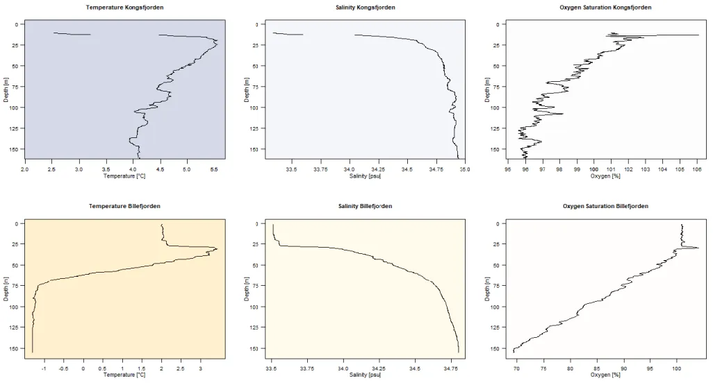
This two-silled fjord is 32 km long and 8-5 km broad, with an outer sill-depth of 70 m and an inner sill depth of 50 m (Figure 5). Its deepest area with approximately 200m is located about 4 km to the tidewater glacier Nordenskiöldbreen. On average, Billefjorden’s main basin has a precipitous topography and is 160 m deep, with a maximum depth of 196 m at its northernmost edge. Szczucinski et al. (2009) found that the hydrography of the fjord is strictly layered during summer with little mixing between layers. They found surface water with a salinity lower than 34 and temperatures above 1°C, intermediate waters of around 34 psu, local fjord water with temperatures from -0.5 to 1°C and slightly higher salinity and below sill depth winter-cooled waters with salinity higher than 34.4 and temperatures lower than -0.5. This unique hydrography distinguishes Billefjorden from other polar fjord-systems and is nowadays rarely found due to ongoing climate change (Figure 2).

13°E 14°E 15°E 16°E 17°E

Billefjorden

(18)

4

Figure 2 Comparison Kongsfjorden and Billefjorden. Upper row: depth profile of Kongsfjorden (04.10.2018) (11.6928°E, 78.9840°N), Lower row: depth profile of Billefjorden (06.10.2018) (16.4997°E, 78.5883°N), plots from left to right: temperature (°C), salinity (psu) and oxygen saturation (%) with increasing depth. (Data from: Mark and Wisotzki 2018).

(19)

5

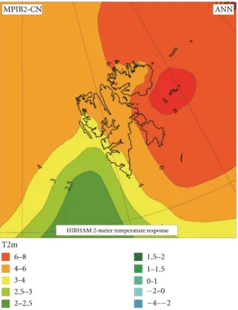
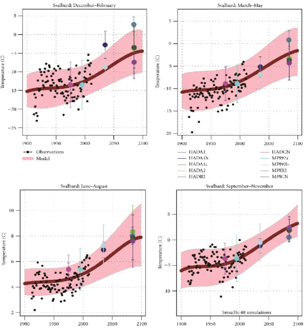
Since industrialization the physicochemical conditions in the world’s oceans changed dramatically. Under ongoing climate change, predicted values for the next hundred years are elevated atmospheric carbon dioxide (CO2) pressure levels up to 1170 μatm; correspondingly the surface water temperatures will increase 2–3 °C, whereas the ocean surface pH will decrease 0.3 – 0.5 units by the year 2100 (Caldeira and Wickett 2005, Meinshausen, Smith et al. 2011, Pörtner, Karl et al. 2014). For the study area of this thesis, Svalbard, Førland et al. (2011) predicted an annual air temperature increase for the whole archipelago of maximum 8 °C and an increase in annual temperature of 4–6 °C in the region of Billefjorden (Figure 3). They moreover predicted winter maximum air temperatures for the year 2050 up to -2.5 °C and for 2100 up to 5 °C, maximum summer air temperatures in 2050 were prognosticated up to 8°C and up to 12 °C in 2100 (Figure 4). An average projected warming in the area of Billefjorden (measured for the Svalbard Airport/Longyearbyen area) from 1961–90 to 2071–2100 corresponded to an increase of 0.6 °C per decade for annual temperatures and a further increase of 0.9 °C per decade in winter is projected for 2071–2100 (Førland, Benestad et al. 2011).

Figure 3 Projected changes from 1961–90 to 2071–2100 in mean annual temperature (°C) The RCM projections are based on MPIB2 (for acronyms, see Appendix Table 12; for weather stations used in the analysis, see Appendix Figure 21) (Førland, Benestad et al. 2011).

(20)

6

Figure 4 Temperature projections for Svalbard Airport/Longyearbyen: results from ESD and RCM downscalings for winter, spring, summer, and autumn. The hatched area (pink) shows 5 % and 95 % interval from ESD estimates, the black dots show observed values, and the thick line (red) show median (50 %) value for the ESD ensemble. The coloured symbols indicate the median value for the different runs with NorACIA-RCM, and the vertical lines show the 5- and 95-percentiles for the RCM runs. The RCM values are plotted on the central year in the respective time slices. (for acronyms, see Appendix Table 12; for weather stations used in the analysis, see Appendix Figure 21) (Førland, Benestad et al. 2011).

Furthermore, the oceans already lost 0.5 - 9 % of their oxygen solubility in cold regions (water temperature around 0 °C) and 0.3 - 5.2 % in tropical regions (40 °C) (Storch, Menzel et al.

2014). Additionally, increasing sea surface temperatures already decreased the sea ice by 49 % compared to the 1979-2000 baseline of 7.0 x 10⁶ km² (Kwok and Untersteiner 2011, Overland and Wang 2013). This sea ice loss can be observed in the fjord systems of the Svalbard archipelago, the study area of this thesis (Nilsen, Cottier et al. 2008, Szczuciński, Zajączkowski

(21)

7

et al. 2009). According to a business-as-usual greenhouse gas emission scenario (RCP8.5) (IPCC 2007), the Arctic is projected to be nearly ice-free in September before the year 2050 (Collins, Knutti et al. 2013). Not only the overall sea ice melting affects the Arctic ecosystem, warming of the western Svalbard fjords due to increasingly warm Atlantic water inflow also causes an overall temperature increase in the Arctic oceans interior (Polyakov, Timokhov et al.

2010). Besides declining sea surface salinities due to freshwater inflow, oxygen loss driven by lowered solubility of O2 in warmer waters and decreased upper ocean stratification challenges marine organisms (Matear and Hirst 2003, Keeling, Körtzinger et al. 2009). Prominska et al.

(2018) showed that winter cooled water is disappearing in warmer years completely out of some fjords, they proved that in Hornsund in the year 2012 winter cooled water was absent in this fjord and the water was dominated by local- and intermediate water. The warmer winter temperatures will reduce the sea ice formation in the fjords, thus no cold, dense, salty, and oxygen-rich water will be formed and the summer stratification will be intensified. As a result, the deep cold water layers do not receive oxygen-rich water and oxygen consumption extends over more than one season. This can lead to local hypoxia in the ground water layers of the protected fjords (Promińska, Falck et al. 2018). Another ecologically important effect of the temperature rise is the invasion of the boreal fish communities into the Arctic regions.

Especially northward migration of predators such as Gadus morhua cause declines in Polar cod stocks (Simpson, Jennings et al. 2011, Renaud, Berge et al. 2012, Kjesbu, Bogstad et al. 2014).

Figure 5 Hydrographic profile along the main axis of Billefjorden (August 2001) A: salinity, B: Water masses are marked by a dotted line, the shaded area marks land masses; SW – surface water, IW – intermediate water, LW – local water, WCW – winter-cooled water (modified after Szczuciński, Zajączkowski et al. 2009).

(22)

8 1.3 Physiological background

In aquatic ecosystems, dissolved oxygen is defined as the primary limiting factor and, together with temperature, dominates physiology as well as behaviour and defines the functional niche of all species (Claireaux and Lefrançois 2007, Pörtner and Knust 2007, Farrell and Richards 2009). For limiting concentrations of dissolved oxygen lower than 2.8 ml/L, the term “hypoxia”

(≙ 39 % air saturation) is defined (Diaz and Rosenberg 1995). According to Henry’s Law (1903), increasing temperatures cause a reduction of oxygen solubility in the oceans. The oceans struggle under the expansion of (hypoxic) oxygen-depleted zones as a consequence of global warming. This oxygen loss affects the thermal tolerance of organisms as described in the concept of oxygen and capacity limited thermal tolerance (OCLTT) (Pörtner and Knust 2007, Pörtner and Lannig 2009, Pörtner, Bock et al. 2017). The concept of OCLTT explains that the capacity of the cardiorespiratory system to maintain the oxygen supply to the tissues sets the tolerance to low and high temperatures, and that these thermal limitations result from the capacity for oxygen supply to the organism in relation to oxygen demand (Pörtner and Knust 2007, Pörtner, Bock et al. 2017).

The “total aerobic excess capacity” is described as a key element for the overall performance of an animal within its thermal range. For the OCLTT concept, the aerobic metabolic scope (AS) is an important parameter to measure thermal stress and to approximate the aerobic performance balance (Pörtner, Bock et al. 2017). It is defined as the difference between minimum and maximum oxygen consumption rate [maximum metabolic rate (MMR) − standard metabolic rate (SMR)] (Pörtner and Lannig 2009). This assumes that there are positive correlations between the AS of an individual and its activity level (Baktoft, Jacobsen et al.

2016). Consequently, the AS is maximized in a defined temperature range to guarantee an optimal fitness (activity) level. The performance of an animal decreases as it is exposed to temperatures beyond or below the pejus temperature range (Tpejus). The AS will decrease until lethal temperatures are reached (Clark, Sandblom et al. 2013). Exhausting exercises are generally accepted to determine the MMR, therefore the critical swimming speed (Ucrit) is experimentally detected, for example under decreasing oxygen (O2) concentration (Brett 1964).

Another method to describe the capacity of fish to maintain aerobic activities is the limiting oxygen level (LOL) curve (Figure 6) (Neill and Bryan 1991, Neill, Miller et al. 1994). The principle is similar to the OCLTT concept as the MMR decreases with decreasing oxygen concentrations until a threshold of critical oxygen concentration (Pcrit) is reached. During the decrease of the MMR, organisms adjust their energy demand in reducing for example their

(23)

9

swimming activity (Domenici, Steffensen et al. 2000, Herbert and Steffensen 2005). When Pcrit

is reached the oxygen content in the water only allows short-term survival and anaerobic metabolism takes place. A further decline in oxygen leads to permanent anaerobic metabolism and a long-time exposure to these conditions to death, depending on the ability of the organism to decrease their SMR (Neill and Bryan 1991, Claireaux and Chabot 2016). The reaction of the organism to decreasing oxygen concentrations can be divided into two groups, either oxygen regulation or oxygen conformity. The metabolic rates of the oxygen regulators decrease in parallel with the decreasing oxygen concentration. As the oxygen concentration decreases, the metabolic rates of the oxygen regulators remain constant for a long time until Pcrit is reached.

When Pcrit is reached, the oxygen regulators switch to oxygen conformers and their metabolic rates also start to decrease as the oxygen saturation continues to decrease below Pcrit. (Ultsch, Jackson et al. 1981, Farrell and Richards 2009, Richards 2009).

Figure 6 Limiting oxygen level (LOL) curve. The ambient oxygen saturation [%] influences the aerobic metabolic capacity of an idealized organism (modified after Claireaux and Chabot 2016).

Shown are the maximum sustainable metabolic rate (MMR) (red dashed line) and standard metabolic rate (SMR) (green dashed line), the LOL curve (black), aerobic scope (distance between LOL curve and SMR) and the critical oxygen level (Pcrit) (Neill and Bryan 1991, Claireaux and Chabot 2016).

To evaluate an animal’s chance of survival under challenging environmental conditions, the SMR is a very important parameter, as it is defined as the minimal level of activity of organisms in total rest, without any muscular activity or even digestion. It only includes the minimal energy costs to sustain life (Krogh 1914).

(24)

10

2

Material and methods

B. saida were caught in October 2018 in Billefjord, Svalbard (Figure 1). They were caught on a research cruise with RV Heincke, Alfred Wegener Institute Helmholtz Centre for Polar and Marine Research, AWI (HE519), using a fish-lift connected to a pelagic trawl at 150m of depth.

The water temperature was -1.5 °C and the oxygen concentration at 150m depth was 5.75 ml/l.

The animals were directly transported to the laboratories of the Alfred Wegener Institute (AWI) in Bremerhaven. They were maintained in two flow-through tanks at normoxia and at an ambient temperature of 0.0 ± 0.5 °C.

An experimental temperature of 2.5 ± 1 °C was chosen for respiration chambers and swim tunnel, according to the thermal window of B. saida (Hognestad 1968, Schurmann and Christiansen 1994, Eriksen, Ingvaldsen et al. 2015, Majewski, Walkusz et al. 2016).

Experimental temperatures were maintained by aid of thermostatted rooms.

2.1 Fish tagging

Before the experiments were started a group of 30 fish between 17 and 23 cm were tagged with passive glass transponders (PIT tag, FDX-B, 7 x 1.35 mm, Loligo Systems Denmark). Before tagging, the fish were anesthetized in a solution of Tricaine methanesulfonate (MS-222) (1 g MS-222 per 8 L seawater). After approximately 3 min in the anaesthetic agent the completely motionless fish was measured (total and standard length, width and depth) and weighted. After that the PIT tag was inserted directly in front of the caudal fin using a disposable syringe needle implanter (Loligo Systems, Denmark) and read by a PIT reader, APR500 (Agrident GmbH, Germany) (Appendix: Table 7). All fish recovered in less than 10 min from this procedure and no later mortality due to tagging and handling stress occurred.

(25)

11 2.2 SMR and RMR measurements

The measurements were taken after Kunz et al. (2018). To ensure standard metabolism, the fish were transferred to the respiration chamber after the seventh day after feeding.

Two fully automated four chamber respirometry systems were used (Complete medium chamber system, Loligo Systems ApS, Denmark). As the ambient water oxygen saturation was measured using one of the oxygen meter ports only seven of the available eight respiration chambers were used in parallel in this experiment. The chambers were submerged in two identical basins, filled with 170 L, connected with U-pipes and one circulating pump. Besides three respiration chambers, one basin contained one oxygen and temperature sensor and the circulating pump, the other contained four chambers. Visual contact between the organisms was prohibited by an impermeable plastic wall between the chambers. For each respiration chamber the PO2 was determined per second using fiber-optic mini sensors (optodes) placed in a probe vessel and connected to a four-channel oxygen meter (Loligo systems ApS, Denmark, Witrox 4 oxygen meter for mini sensors). The optodes were calibrated within the experimental set-up by flushing the basins with nitrogen to set for 0 % oxygen saturation and then calibrated for 100 % O2 saturation in completely oxygen-saturated seawater. Due to calibration problems, some of the recorded oxygen values (100 – 5 %) had to be recalculated using a new 0 % calibration. Following a recalibration, the measurements at 10 and 5% were repeated with the correct 0% calibration (Troubleshooting is described under 2.4.9). The automated intermittent respirometry software, AuroResp (version 2.3.0, Loligo Systems ApS, Denmark) was used to acquire the oxygen saturation and temperature data within the chambers and control oxygen saturation in the basins and water flow though the chambers. Intermittent flow was chosen in this study. A measurement period of 30 min (only recirculation pumps working) was followed by a short waiting period of 30 sec and a 5 min long flushing phase (only flush pumps working).

(26)

12

Figure 7 Schematic construction of the respirometry system. All respiration chambers are connected to one recirculation pump and one flush pump. Within the recirculating water, flow probe vessels are included where the oxygen probes are located. A four-channel oxygen meter (Loligo systems ApS, Denmark, Witrox 4 oxygen meter for mini sensors) detects the ambient oxygen in the chambers and basin as well as temperature, sending the data via Bluetooth to a computer with the software AutoResp version 2.3.0 (Loligo Systems ApS, Denmark). Compressed air (CA) together with nitrogen (N2) create the desired oxygen concentration (100 - 5 % saturation). The data acquisition instrument (DAQ-M) controls the flush and recirculation pumps and the amount of nitrogen pumped into the water.

DAQ-M is also connected to and controlled by a computer with the software AutoResp.

In the beginning of this study, eight different PO2 steps were determined by a short initial experiment with seven individuals. After an initial oxygen saturation of 100 % was reached the flushing pumps were shut off, switching from intermitted flow to closed mode. The metabolic rate was calculated by the AutoResp software and graphically displayed. Consequently, the metabolic rate decreased with diminishing oxygen saturation and a possible Pcrit (critical oxygen saturation) was determined. All fish performed well until 15-10 % oxygen saturation was reached. Compared to literature values for other Gadidae species the expected Pcrit was assumed to be around 30 %. Therefore, the PO2 steps for this experiment were chosen as follows to detect the exact Pcrit for this species: 100, 75, 65, 50, 40, 30, 25, 20, 15, 10 and 5 % oxygen saturation.

The desired oxygen concentration was maintained by constant gassing with compressed air and additional nitrogen, controlled by the AutoResp software. Each oxygen saturation was maintained for two days and two nights, containing approximately 80 measurement phases.

CA

(27)

13

The rates of oxygen consumption were calculated after Boutilier et al. (Boutilier, Heming et al.

1984) and normalized after Steffensen et al. (Steffensen, Bushnell et al. 1994) (see below: 2.5.

Data handling) using the statistical software “R” (package “FishResp” and “Mclust”).

All chambers were cleaned weekly. For this purpose, they were removed from the experimental setup, rinsed with tap water, wiped out and set up to dry for two days.

2.3 Swimming performance measurements

The metabolic rate and swimming performance of B. saida under hypoxia were recorded following a critical swimming speed (Ucrit) protocol (Brett 1964). The following PO2 steps for this experiment were selected: 100, 70, 60, 50, 40, 30, 25, 20, 15 and 10 % oxygen saturation.

A sample size of six individuals was chosen for each PO2 treatment.

A Brett-type swim tunnel respirometer of 5l (30 x 7,5 x 7,5 cm, Loligo Systems ApS, Denmark) was used to measure the swimming performance of B. saida (n=6 per treatment). To control the oxygen content and flushing phases, a DAQ-M instrument (Loligo Systems ApS, Denmark) was added to the system. The swim tunnel was submerged in a reservoir tank to maintain stable abiotic conditions within the chamber. The water velocity was regulated by a control unit regulating the engine controlling a propeller within the swim chamber (Loligo Systems ApS, Denmark). To calibrate the water velocity to voltage output from the control system, a flow sensor was used (Appendix: Figure 18). The PO2 was determined using fiber optic mini sensors (optodes) connected to a four-channel oxygen meter (Loligo systems ApS, Denmark, Witrox 4 oxygen meter for mini sensors). The measurements were taken after Kunz et al. (2018). The desired oxygen concentration was maintained by constant gassing with compressed air and additional nitrogen, controlled by the AutoResp software.

(28)

14

Figure 8 Schematic construction of the swim tunnel A four-channel oxygen meter (Loligo systems ApS, Denmark, Witrox 4 oxygen meter for mini sensors) detects the ambient oxygen in the swim tunnel as well as temperature, sending the data via Bluetooth to a computer with the software AutoResp version 2.2.0 (Loligo Systems ApS, Denmark). Compressed air (CA) together with nitrogen (N2) create the desired oxygen concentration (100 – 10 % oxygen saturation). The data acquisition instrument (DAQ-M) controls the flush pump and the amount of nitrogen pumped into the water. DAQ- M is also connected to and controlled by a computer with the software AutoResp. A motor regulated by the controller drives the propeller, creating a laminar current within the swim tunnel. The fish is placed in the operation part of the tunnel.

Seven days after feeding the fish were transferred to the swim tunnel. In order to minimize air contact and possible oxygen stress, the fish were placed in the swim tunnel with a water-filled plastic bag. After an acclimatization period of 30 min the propeller was turned on and the fish were pre-conditioned to a water velocity of 1.2 BL (body length)/sec for 1 h and 25 min.

Afterwards the velocity was increased to the first measurements velocity of 1.4 BL/sec for 5 min before the Ucrit protocol started. This method was established to produce more robust swimming trials (Reidy, Kerr et al. 2000). A white plastic cover was used to minimize effects of disturbance. Subsequently, the Ucrit protocol began at 1.4 BL/sec. The water velocity was increased by 0.15 BL/sec every 11 min. The flushing pump was switched on according to the velocity steps. A 30 second long flushing phase started after 11 min, when a specific velocity interval was over. After that a 30 second waiting period took place and then 10 min of measuring time followed to record oxygen consumption. To determine the gait‐transition speed (Ugait: the speed at which the fish changes from strictly pectoral to pectoral‐and‐caudal swimming) (Heglund, Taylor et al. 1974, Heglund and Taylor 1988, Drucker and Jensen 1996)

CA

(29)

15

the kick-and-glide swimming style (bursts) (Videler 1981) were documented. In kick-and-glide swimming, thrust generation is supplemented by anaerobic muscle contractions and mainly the white muscles are used. All bursts were counted and the corresponding time was documented.

The water velocity was stepwise increased until the fish was exhausted. This was defined as the point at which a fish completely refused to swim and was inactive for more than three minutes.

The critical swimming velocities (Ucrit) of the fish were calculated as described by Brett (1964) (see: 2.4.7). After Ucrit was reached the velocity was immediately decreased to the basic weaning velocity of 1.4 BL/sec for another 10 min the fish stayed in the swim tunnel.

Afterwards the fish were set back into their collection tank. The maximum metabolic rate was determined under each oxygen saturation inside the swim tunnel, similar to the approach described for the respiration chambers above.

The swim tunnel was cleaned at the end of each day. For this purpose, the old water was removed from the swim tunnel, the tunnel was wiped dry and filled with fresh, pre-cooled sea water. All loose parts were also removed from the tunnel, flushed with tap water, wiped dry and returned to the swim tunnel.

2.4 Data handling

2.4.1 Oxygen consumption

The metabolic rates (M_O2) were calculated using the R package “FishResp” on the basis of this equation:

MO₂= ∆PO2 ∙ V ∙ α ∙ M⁻¹∙ ∆t⁻¹ (1)

where ∆PO2is the change in water PO2(kPa), V is the volume of the respirometer (l) less the volume of the fish (l), α is the O2 solubility coefficient after Boutilier et al. (1984), M is mass of fish (kg) and ∆t is the elapsed time (h).

(30)

16 2.4.2 Normalized oxygen consumption

The M_O2data was normalized using R package “FishResp” on the basis of this equation:

𝑀_𝑂₂ = 𝑀_𝑂_2(𝑙)∙ (^𝐵𝑊

100)^(1−𝐴) (2)

with MO2(100)is the oxygen consumption for a 100g fish, MO2(I)is the oxygen consumption for a fish with a certain body weight (g) (BW), and A is the mass exponent describing relationship between metabolic rate and BW. As A, 0.8 will be used after Steffensen et al. (1994) and Holeton (1974).

2.4.3 Standard metabolic rate

The SMR was calculated after Chabot et al. (2016) in R, using the package “Mclust”. Only the data of the respiration chambers were used. Of these, only the data from the treatments 60 %, 70 % and 100 % were used for calculation, as in this oxygen range the metabolic rates of fish used to be stable. The lower 5 % of these data were removed as outliers, then a mean value of the remaining lower 15 % could be determined. This value was determined as SMR (Chabot, Steffensen et al. 2016).

2.4.4 Routine metabolic rates

The RMR was calculated in R. The metabolic rates recorded in the respiration chambers were grouped by treatments (5 - 100 % PO2). For each fish within a PO2 group, approximately 45 individual metabolic rates were calculated. After the lowest 5 % metabolic rates of each fish within a treatment were discarded as outliers, the mean value of the remaining lowest 15 % of each fish in the corresponding treatment was calculated and assumed as RMR of the respective fish. The mean value of all calculated RMRs in a treatment was calculated and taken as the RMR for that specific treatment. The standard deviation was calculated for each PO2 group.

(31)

17 2.4.5 Maximum metabolic rates

Due to the short measuring time of maximum two hours, the number of measuring points per fish (between 3 and 10 individual metabolic rates) was too small to calculate the mean value of the highest 15% for each fish after the highest 5% were removed as outliers. Therefore, before determining the MMR, the highest 5% of all recorded metabolic rates of the swim tunnel experiment were removed as outliers. The remaining highest metabolic rate per fish was taken as MMR. The mean value of all individual MMRs in one treatment was calculated. The standard deviation was calculated for each PO2 group.

2.4.6 Aerobic scope

The aerobic scope is defined as:

AS = MMR − SMR (3)

In this study, only one RMR could be calculated for each fish and treatment. Since a state of complete immobility and dormancy of the organisms could not be achieved by the stay in the experimental set-up and therefore a RMR rather than a SMR has taken place. Therefore the AS was calculated as follows:

AS = MMR − RMR (4)

All possible combinations between RMR (2.4.4) MMR (2.4.5) were calculated in R using the package “tidyr”, the differences between the newly paired RMR and MMR combinations within one PO2 treatment (10 - 100 %) were calculated and a standard deviation was determined.

2.4.7 Critical swimming speed (Ucrit) after Brett (1964)

The critical swimming speed was adjusted as:

𝑈_crit= 𝑈_𝑚𝑎𝑥+ ^𝑣𝑇

𝑡 (5)

In this equation Umax is the highest velocity (v) perpetuated for a complete time interval (t) and T is the time spent at the given velocity leading to exhaustion of the fish.

(32)

18 2.4.8 Gait transition speed (Ugait)

The critical swimming speed was adjusted as:

𝑈_gait = 𝑈_𝑚𝑎𝑥+ ^𝑣𝑇

𝑡 (6)

In this equation Umax is the highest velocity (v) perpetuated for a complete time interval (t) without bursting and T is the time spent at the given velocity leading to bursting of the fish.

2.4.9 Troubleshooting

Due to calibration problems (initial drift of 0 % calibration), some of the recorded oxygen values (100-5 %) had to be recalculated using a new 0 % calibration. After a new 0 % calibration was performed these calibration values were used to recalculate the recorded oxygen concentrations with the PreSens Oxygen Calculator (version 3.1.1, PreSens Precision Sensing GmbH, Germany). Therefore, the data had to be converted to an excel-file written with PreSens Measurement Studio 2 (version 3.0.1, PreSens Precision Sensing GmbH, Germany). This program detects all calibration coefficients of an optical oxygen sensor, needed to recalculate the data, automatically. In PreSens Measurement Studio 2 short measurement files with the identical oxygen optodes used in the main experiment were performed. After that the raw data from AutoResp were inserted into this data file. All values as partial pressure, salinity and temperature were transferred to the new file as well. Afterwards this file could be recalculated with the calculator. For this purpose the new calibration values for the corresponding optode had to be entered in the software. The calculator returned a new file with corrected values which could be used to calculate the correct metabolic rate (using the R package “FishResp”).

2.4.10 Statistical analysis

The normal distribution of the data was determined using the Shapiro-Wilk test or the Kruskal- Wallis test. The homoscedasticity was evaluated with the Levene test. The differences between PO2 treatments were evaluated with a one-way (respirometry chambers, burst counts and swimming time) or two-way ANOVA (swim tunnel) followed by Tukey’s test for mean value comparison. Furthermore, the influence of body weight, body length, temperature and water velocity were examined. The level of statistical significance was set at p<0.05 for all statistical tests. All statistical tests were performed with R 3.6.1.

(33)

19

3

Results

3.1 Mortality

Within the experimental setups, Polar cod mortality occurred solely at the lowest PO2 treatment in respiration chambers. Two Polar cod died during the acclimation phase, the first night after they were placed in the chambers. Another four individuals died in the holding aquarium, independent of the handling stress.

3.2 Respiration measurements

All measurements were significantly influenced by individual body weight (pRMR < 0.0001, pMMR = 0.0039). A significant temperature effect only occurred in the respiration chambers (p

< 0.0001). The temperature differed between 2.2 and 3.2 °C, with a mean temperature of 2.68

± 0.25 °C. The MMR was significantly influenced (p = 0.0082) by individual body lengths as well. The swim tunnel measurements were maintained at a temperature of 1.23 ± 0.34 °C

3.2.1 Standard metabolic rate

The SMR of B. saida was calculated after Chabot et al. (2016) (see 2.4.3) using the lower 15 % quantile of the metabolic rates recorded under 60-100% oxygen saturation in respiration chambers. This includes metabolic rates of 29 individuals. The calculated SMR of Polar cod was 0.44 µmol O2/g∙h.

Figure 9 Standard metabolic rate (SMR). Shown are the metabolic rates ((MR) in µmol O2/g∙h) (orange circles) recorded at 56 - 100 % PO2. The SMR (0.44µmol O2/g∙h; black line) was calculated as described under point 2.4.3 using the R package “Mclust” after Chabot et al. (2016).

(34)

20 3.2.2 Standard and routine metabolic rate

After fish were placed in the respiration chambers their oxygen consumption declined during the first 36 h, reaching a steady level afterwards. Therefore, the measurements recorded within the second night were used in this study, when fish had been in the respirometer setups for an average of 36 h.

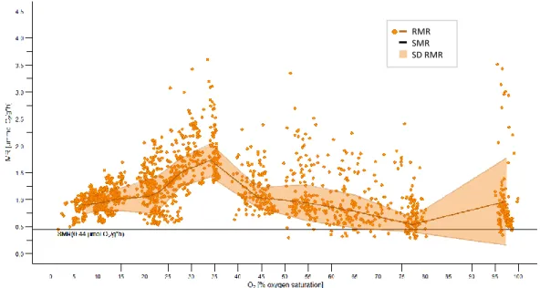
The metabolic rates were significantly dependent on PO2 (p= <2e-16). The calculated RMR (Figure 10, Table 1) remained on a similar level between 100 and 45 % PO2 (max: 0.97 ± 0.81, min: 0.53 ± 0.13 µmol O2/g∙h), below which oxygen consumption slightly increased between 45 and 35 % oxygen saturation up to 1.78 ± 0.35 µmol O2/g∙h (p < 0.0001). From 35 to 20 % oxygen saturation the metabolic rate decreased constantly down to 1.06 ± 0.31 µmol O2/g∙h (p

< 0.0001). Between 20 and 5 % oxygen saturation the oxygen consumption remained stable and did not decrease below the SMR level. The minimum routine metabolic rate reached in this experiment was 0.86 ± 0.14 µmol O2/g∙h at 10.97 ± 0.92 % PO2.

Figure 10 Routine metabolic rate (RMR). Shown are the metabolic rates ((MR) in µmol O2/g∙h) (orange circles) (86 experimental runs representing 1887 single metabolic rate data points of 30 individuals) performed between 5 and 100 % PO2 in respiration chambers. The RMR (dark orange line, with SD (light orange area)) was calculated as described under point 2.4.4. Black line: standard metabolic rate (SMR; 0.44 µmol O2/g∙h).

RMR SMR SD RMR