IHS Economics Series Working Paper 326
January 2017
Exchange rate forecasting and the performance of currency portfolios
Jesús Crespo-Cuaresma Ines Fortin Jaroslava Hlouskova
Impressum Author(s):
Jesús Crespo-Cuaresma, Ines Fortin, Jaroslava Hlouskova Title:
Exchange rate forecasting and the performance of currency portfolios ISSN: 1605-7996
2017 Institut für Höhere Studien - Institute for Advanced Studies (IHS) Josefstädter Straße 39, A-1080 Wien
E-Mail: o ce@ihs.ac.atffi Web: ww w .ihs.ac. a t
All IHS Working Papers are available online: http://irihs. ihs. ac.at/view/ihs_series/
This paper is available for download without charge at:
https://irihs.ihs.ac.at/id/eprint/4175/
Exchange rate forecasting and the performance of currency portfolios
∗Jesus Crespo Cuaresma
Department of Economics, Vienna University of Economics and Business (WU), Austria Wittgenstein Centre for Demography and Global Human Capital (WIC), Austria
World Population Program, International Institute for Applied Systems Analysis (IIASA), Austria Austrian Institute of Economic Research (WIFO), Austria
Ines Fortin
Research Group Financial Markets and Econometrics, Institute for Advanced Studies, Vienna, Austria
Jaroslava Hlouskova
Research Group Financial Markets and Econometrics, Institute for Advanced Studies, Vienna, Austria Department of Economics, Thompson Rivers University, Kamloops, BC, Canada
Abstract
We examine the potential gains of using exchange rate forecast models and forecast com- bination methods in the management of currency portfolios for three exchange rates, the euro (EUR) versus the US dollar (USD), the British pound (GBP) and the Japanese yen (JPY). We use a battery of econometric specifications to evaluate whether optimal currency portfolios implied by trading strategies based on exchange rate forecasts out- perform single-currency and the equally weighted portfolio. We assess the differences in profitability of optimal currency portfolios for different types of investor preferences, different trading strategies, different composite forecasts and different forecast horizons.
Our results indicate that the benefits of integrating exchange rate forecasts from state- of-the-art econometric models in currency portfolios are sensitive to the trading strategy under consideration and vary strongly across prediction horizons.
Keywords: currency portfolios, exchange rate forecasting, trading strategies, profitability JEL classification: G02, G11, E20
∗Ines Fortin and Jaroslava Hlouskova gratefully acknowledge financial support from Oesterreichische Na- tionalbank (Anniversary Fund, Grant No. 16250).
1 Introduction
Foreign exchange risk is omnipresent in international portfolio diversification, but forecasting exchange rates is well known to be a difficult task. Since the seminal work by Meese and Rogoff (1983), which shows that econometric specifications based on macroeconomic fundamentals are unable to outperform simple random walk forecasts at short time horizons (up to one year), a large number of studies have proposed models aimed at providing accurate out-of- sample predictions of spot exchange rates (see MacDonald and Taylor, 1994; Mark, 1995;
Chinn and Meese, 1995; Kilian, 1999; Mark and Sul, 2001; Berkowitz and Giorgianni, 2001;
Cheung et al., 2005; or Boudoukh et al., 2008, among others). In parallel, a literature has emerged which examines empirically the potential profitability of technical trading rules based on exchange rate predictions (see Menkhoff and Taylor, 2007, for a review). Although the random walk specification has naturally emerged as the benchmark to beat in terms of out- of-sample predictive accuracy, it is not clear that it will also yield the most profitable trading strategy. Portfolio managers are expected to be more concerned with profitability than with out-of-sample accuracy.
Our study takes the perspective of a currency portfolio manager (investor) who follows trading strategies based on exchange rate forecasts and whose main goal is to maximize (risk- adjusted) profits, under certain types of preferences. More specifically, our currency portfolio manager considers the exchange rates of the euro against the US dollar, the British pound and the Japanese yen and, for each of these three exchange rates, creates a ‘single asset’. The returns of this asset are implied by a certain trading strategy that is based on exchange rate forecasts. The optimal portfolio is then made up of these three single assets according to the manager’s – or some investor’s – preferences.
The two primary research questions in our study are the following. First, does the optimal currency portfolio outperform some simpler benchmark portfolios and thus is there a value added in engaging in active portfolio management – or can the portfolio manager achieve the same (risk-adjusted) profit by just investing in some simpler assets (benchmark portfolios)?
As simpler assets we consider the single assets of which the optimal portfolio consists as well as the equally weighted portfolio based on forecasts from the model as well as on random walk predictions. These benchmark portfolios would not require active portfolio management and thus would represent substantially simpler investment strategies. Second, how do the different optimal currency portfolios (constructed according to different types of preferences, different trading strategies, different composite forecasts and different forecast horizons) compare to each other and is there one optimal portfolio which systematically outperforms the others?
Relating to the first research question, we find some evidence indicating that simpler portfolios, like equally weighted portfolios, are not necessarily outperformed (e.g., in terms of the Sharpe ratio) by more complex portfolios (see DeMiguel et al., 2009 and Jacobs et al., 2014). The existing evidence in the literature, however, relates to equity markets (DeMiguel
et al., 2009) and equity, bond and commodity markets (Jacobs et al., 2014), and it is not obvious that these findings carry over to foreign exchange markets. Our study contributes to enlarge this body of empirical evidence by concentrating on foreign exchange markets.
In order to compare the different currency portfolios, we employ a number of (risk- adjusted) performance measures, including the Omega measure, the Sharpe ratio and the Sortino ratio. In order to generate the exchange rate forecasts, we consider all the multivari- ate time series models and the methods of forecast combinations entertained in Costantini et al. (2014, 2016).1 While they examine exclusively the predictability of individual exchange rates2 in terms of out-of-sample accuracy, directional accuracy and profitability of trading strategies, we go a step further and build optimal currency portfolios, which we analyze in terms of risk-adjusted profitability. In order to generate the out-of-sample exchange rate forecasts required for the trading strategies, we also employ averaged predictions based on different loss and profit measures over a certain time span (mean-squared-error, directional value and returns) leading to different so-called composite forecasts. As far as the forecast horizon is concerned, we look at horizons of one month and three months. To obtain optimal portfolios, we consider a wide range of different types of preferences, including the mean- variance investor, the conditional value-at-risk investor, the linear investor, the linear loss aversion investor and the quadratic loss aversion investor. These preferences are also used, e.g., in Fortin and Hlouskova (2011) and Fortin and Hlouskova (2015). While these pieces of research investigate optimal asset allocation among sectoral stock indices, government bonds and commodities, we look here solely at assets based on trading strategies applied to different exchange rates.
In order to assess the performance of optimal currency portfolios versus benchmark port- folios (single assets, equally weighted portfolio), we use a data snooping bias free test, which is based on an extensive bootstrap-procedure. By employing this test we want to ensure that the performance superiority of certain optimal portfolios – if any – is systematic and not merely due to luck. The test identifies which optimal portfolios significantly beat the benchmark portfolio in terms of certain risk-adjusted performance measures.
We look at two different trading strategies in constructing the single assets. The first one is the simple ‘buy low, sell high’ trading strategy described, e.g., in Gen¸cay (1998), where the trading signal is based on the spot exchange rate and its forecast. The second one is based on exploiting the forward rate unbiased expectation hypothesis and is similar to the carry trade strategy (implemented using forward contracts) used, e.g., in Burnside et al. (2008). In this case the trading signal is based on the forward exchange rate and the exchange rate forecast.
Returns implied by trading strategies have also been investigated in other exchange rate
1See also Crespo Cuaresma and Hlouskova (2005), Crespo Cuaresma (2007), Costantini and Pappalardo (2010) and Costantini and Kunst (2011).
2Costantini et al. (2014) consider the euro against the US dollar, the British pound, the Swiss franc and the Japanese yen, Costantini et al. (2016) consider the euro against the US dollar.
studies. Burnside et al. (2008), for example, examine the returns implied by the carry trade strategy, which determines to sell (buy) a currency forward when it trades at a forward pre- mium (discount). This trading strategy is similar to our second trading strategy. The authors apply the carry trade strategy to individual currencies as well as to an equally weighted port- folio of 23 currencies and find that that constructing a portfolio improves the performance of the carry trade strategy substantially: the Sharpe ratio of the equally weighted carry trade strategy is more than 50% higher than the median Sharpe ratio across currency specific carry trade strategies. Unlike our study, Burnside et al. (2008) do not test the statistical signifi- cance of the portfolio outperformance with respect to the single currency based asset. While they use a simple, equally weighted portfolio, we take the investor’s preferences into account explicitly and optimize the portfolio according to these preferences. Another fundamental difference with respect to their work is that we include exchange rate forecasts in the def- inition of our trading strategies with the aim of improving their performance. Burnside et al. (2008), on the other hand, use bid and ask spot and forward exchange rates. In a re- lated paper, Burnside et al. (2011) examine carry trade and momentum strategies for single currencies and equally weighted currency portfolios, and review possible explanations for the profitability of these strategies.
There are only few existing studies which explicitly deal with optimal currency portfolios.
Recently, the work by Barroso and Santa-Clara (2015) aims at maximizing the expected return of a portfolio in the forward exchange market, given preferences described by the power utility and using the parametric portfolio policies approach of Brandt et al. (2009). This approach models the asset weights as a function of their characteristics, and the relevance of these characteristics in forming portfolios is the focus of the study. The authors find that carry, momentum, and value reversal contribute to portfolio performance, whereas the real exchange rate and the current account do not. They argue that besides risk, currency returns reflect the scarcity of (speculative) capital. The study is related to ours since it deals with currency portfolio optimization according to given preferences, however, the focus – and also the assets from which portfolios are built – are very different.
Another paper dealing with currency portfolio optimization, using the mean-variance ap- proach, is by Papaioannou et al. (2006). The authors are mainly interested in how the introduction of the euro as a new currency has changed, if at all, the optimal composition of portfolios of foreign exchange reserves and how the optimal holdings compare to actual reserve portfolios held by central banks. The expected returns in the different currencies depend on the domestic interest rates and the expected changes in foreign exchange rates. Except for the random walk forecast, no exchange rate forecasts are used in the analysis, while in our study exchange rate forecasts are one of the central ingredients of the analysis. The authors find, among other results, that the optimal shares in the US dollar match its large shares in actual foreign reserves and that the optimal euro shares are much smaller that the shares
observed. The optimization results are sensitive to the reference currency, which – for the main analysis – is the US dollar.
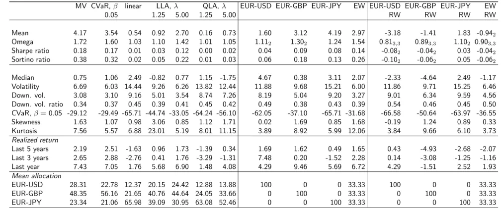
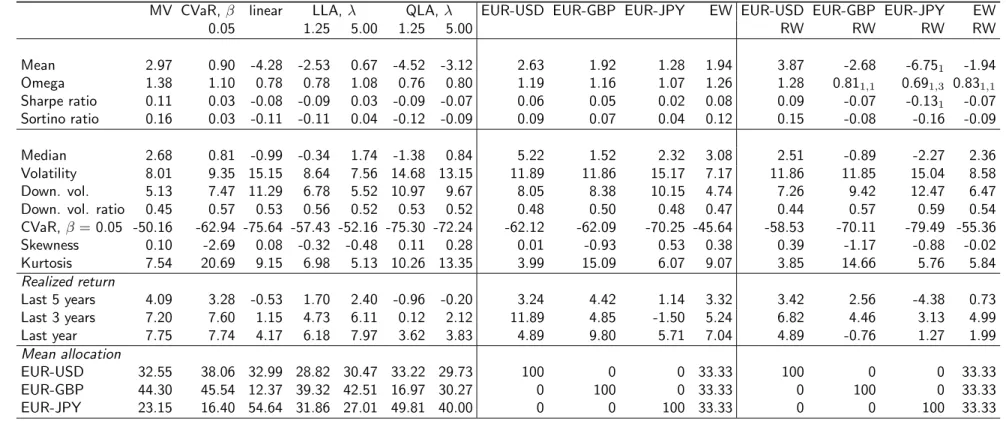
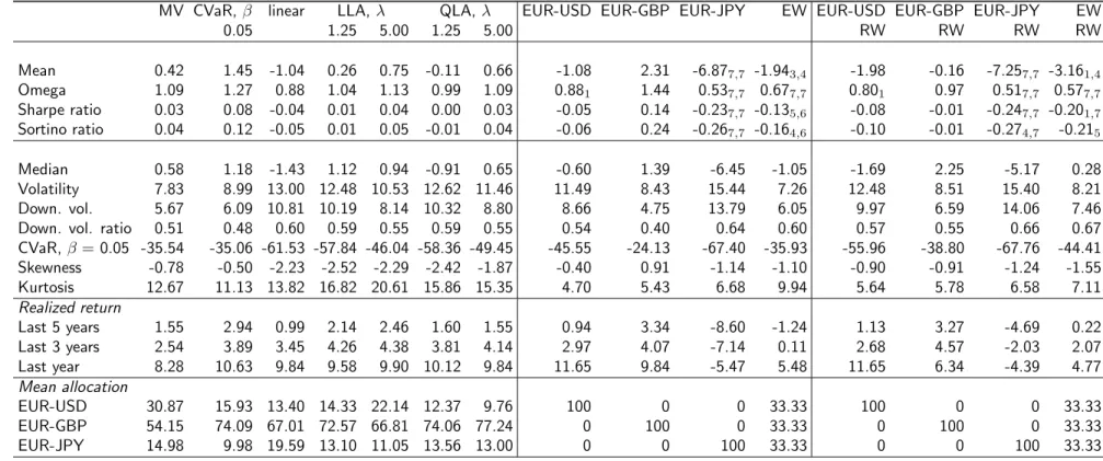
Our analysis reveals that for a forecast horizon of one month, the mean-variance currency portfolio outperforms the single asset based on the EUR/JPY exchange rate in terms of the Omega measure, for all three composite forecasts. The equally weighted portfolio, however, is never outperformed for this forecast horizon. For a forecast horizon of three months, on the other hand, the equally weighted portfolio is always outperformed (for all composite forecasts and both trading strategies) – and most often not only in terms of the Omega measure but in terms of all four performance measures. This is also true for longer forecast horizons (six and twelve months). In general, the benchmark portfolios based on the random walk, i.e., the benchmark portfolios which do not make use of any (non-trivial) exchange rate forecasts, are more often outperformed than the benchmark portfolios based on composite forecasts.
For a given trading strategy and a given composite forecast, the best and second best performances (in terms of the mean return, the Omega measure, the Sharpe ratio and the Sortino ratio) are mostly achieved by the mean-variance and conditional value-at-risk port- folios. This is true for both the forecast horizon of one month and the forecast horizon of three months. For forecast horizons of six and twelve months, however, also the linear and quadratic loss aversion portfolios are among the best and second best performing portfolios.
For a given type of investor and a given composite forecast, the ‘buy low, sell high’ strategy shows the better performance, with only few exceptions. This is true for forecast horizons of one, three, six and twelve months. Note that for a forecast horizon of three months and directional-value-based composite forecasts, the difference between the ‘buy low, sell high’
strategy and the carry trade based strategy is quite substantial. In general, the optimal portfolio performance and its allocation seems to be quite sensitive to the trading strategy under consideration.
For a given type of investor and a given trading strategy, the MSE-based composite forecast yields the best performance, provided the forecast horizon is one month. For a forecast horizon of three months, however, best performances are rather achieved by directional-value-based and return-based composite forecasts.
The paper is structured as follows. In Section 2 we present the analytical framework required for exchange rate forecasting and portfolio optimization. First we introduce the individual exchange rate forecast models and forecast combinations methods which we use to generate the exchange rate predictions. Then we describe the loss and profit measures employed to compute the best forecasts (and thus the composite forecasts). The different types of preferences and the corresponding optimization problems are presented. We conclude Section 2 by describing the data snooping bias free test for equal performance and presenting the risk-adjusted performance measures we consider. Section 3 discusses the empirical results, first for the forecast horizon of one month and then for the forecast horizon of three months.
Section 4 concludes.
2 Analytical framework: Exchange rate forecasting and opti- mal currency portfolios
2.1 Exchange rate specifications
We start by describing the modelling framework used to obtain ensembles of exchange rate predictions which can then be used to construct currency portfolios. The class of specifica- tions we entertain in order to obtain forecasts of the exchange rate can be conceptualized in the context of the so-called monetary model of exchange rates originally developed in the work by, for example Frenkel (1976), Dornbusch (1976) or Hooper and Morton (1982). The monetary model of exchange rate determination has been often used as a theoretical frame- work to create exchange rate predictions based on macroeconomic fundamentals (see Crespo Cuaresma and Hlouskova, 2005; Costantini et al. 2016). Starting with standard Cagan money demand equations for the domestic and foreign economy, the monetary model of exchange rate formation assumes that purchasing power parity acts as a long-run equilibrium and thus leads to a relationship between the exchange rate on the one hand and the money supply levels, interest rates and income levels in the two economies on the other hand.
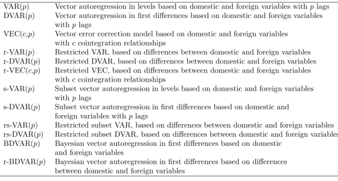
Such a relationship tends to be routinely specified empirically in the form of vector au- toregressive (VAR) and vector error-correction (VEC) models. Defining the vectoryt, which contains the (log) exchange rate, the (log) money supply in the domestic and foreign economy, the (log) production index in the domestic and foreign economy and the respective short and long term interest rates, this implies that its dynamics are given by
yt= Φ0+
p
X
l=1
Φlyt−l+εt, εt∼NID(0,Σε), (1) where Φl for l= 1, . . . , pare matrices of coefficients and Φ0 is a vector of constants. Alter- natively, if the variables of the model are linked by one or more cointegration relationships which act as a long-run attractor of the data, the specification given by equation (1) can be written in vector error correction (VEC) form,
∆yt= Θ0+δψ′yt−1+
p−1
X
l=1
Θl∆yt−l+εt. (2)
In this specification the cointegration relationships are given by ψ′yt and δ quantifies the speed of adjustment to the long-run equilibrium. Alternatively, if the variables in yt are unit-root nonstationary but no cointegration relationship exists among them, a VAR model in first differences (DVAR) would be the appropriate representation, which amounts to the
model given in equation (2) withδ = 0.
2.2 Forecast combinations
The set of methods used to create forecast combinations from individual multivariate time series models are similar to those in Costantini et al. (2016). Let Stj be the spot exchange rate of euros (EUR) per foreign currency unit (FCU) of currencyj, i.e., EUR/FCU, at timet, and let ˆSm,t+h|tj be the exchange rate forecast of euros per foreign currency unit of currencyj obtained using modelm,m= 1, . . . , M,for timet+hconditional on the information available at timet (i.e., h is the forecast horizon). In the following we drop superscript j to keep the exposition simpler. The combinations of forecasts entertained in this study, ˆSc,t+h|t, take the form of a linear combination of the predictions of individual specifications,
Sˆc,t+h|t=whc,0t+
M
X
m=1
wc,mth Sˆm,t+h|t, (3)
where c is the combination method, M is the number of individual forecasts, and the weights are given by{wc,mth }Mm=0.
Since several combination methods require statistics based on a hold-out sample where the relative predictive ability of models is assessed, let us introduce here some notation on subsample limits: T0 is used to denote the first observation of the available sample, the interval (T1,T2) is used as a hold-out sample to obtain weights for those methods where such a subsample is required, and T3 is the last available observation. The sample given by (T2, T3) is the proper out-of-sample period used to compare the different methods.
In order to pool the forecasts of individual specifications, we consider a large number of combination methods proposed in the literature. These are the same methods have been recently used in Costantini et al. (2016) to evaluate exchange rate predictability:3
• Mean, trimmed mean, median. For the mean prediction, whmean,0t = 0 andwmean,mth =
1
M in equation (3). The trimmed mean uses whtrim,0t = 0 and wtrim,mth = 0 for the individual models that generate the smallest and largest forecasts, whilewhtrim,mt= M−21 for the remaining individual models. For the median combination method, ˆSc,t+h|t = median{Sˆm,t+h|t}Mm=1 is used (see Costantini and Pappalardo, 2010).
• Ordinary least squares (OLS) combination. Weights of this method coincide with es- timated coefficients obtained by regressing actual exchange rates on a constant and corresponding exchange rate forecasts. In our application we use a rolling window over the hold-out sample. Granger and Ramanathan (1984) provide more detail on this simple forecast pooling methodology.
3Costantini et al. (2016) provide a more detailed discussion of these forecast averaging methods.
• Combination based on principal components (PC). This method allows to overcome multicollinearity of predictions across models by reducing them to a few principal com- ponents (factors). The method is identical to the OLS combining method by replacing forecasts with their principal components. In our application, we choose the number of principal components using the variance proportion criterion, which selects the smallest number of principal components such that a certain fraction of variance is explained.
We set the proportion to 80%.4
• Combination based on the discount mean square forecast errors (DMSFE). Following Stock and Watson (2004), the weights in equation (3) depend inversely on the historical forecasting performance of individual models,
wDMSFE,m,th = WMSE−1mth PM
l=1WMSE−1lth, (4)
where
WMSEmth =
t
X
˜t=T1−1+h
θT−h−˜t
S˜t+h−Sˆm,˜t+h|˜t2
, (5)
for t=T2−h, . . . , T3−h,m= 1, . . . , M, whDMSFE,0,t = 0 andθis a discount factor. In the empirical application, we use θ= 0.95.
• Combination based on hit/success rates (HR). The method uses the proportion of cor- rectly predicted directions of exchange rate changes of model m to the number of all correctly predicted directions of exchange rate changes by the models entertained,
wHR,mth =
Pt
˜t=T1+h−1DAm,˜th PM
l=1
Pt
j=T1+h−1DAl,˜th (6)
wheret=T2−h, . . . , T3−hand the index of directional accuracy is given byDAm,th= I
sgn(St−St−h) = sgn( ˆSm,t|t−h−St−h)
, whereI(·) is the indicator function.
• Combination based on the exponential of hit/success rates (EHR)(Bacchini et al., 2010).
The weights in this method are obtained as
wEHR,mth =
exp Pt
t=T˜ 1+h−1(DAm,˜th−1) PM
l=1exp Pt
˜t=T1+h−1(DAl,˜th−1) (7) where t=T2−h, . . . , T3−h.
4More details on the method are provided in Hlouskova and Wagner (2013), where the principal components augmented regressions are used in the context of the empirical analysis of economic growth differentials across countries. Except for Costantini et al. (2016), we are not aware of the existence of any study using this approach in the context of the exchange rate forecasts.
• Combination based on the economic evaluation of directional forecasts (EEDF). The weights in this method capture the ability of models to predict the direction of change of the exchange rate while also taking into account the magnitude of the realized change,
whEEDF,mt =
Pt
˜t=T1+h−1DVm,˜th PM
l=1
Pt
˜t=T1+h−1DVl,˜th (8) where t=T2−h, . . . , T3−h andDVm,th=|St−St−h|DAm,th.
• Combination based on predictive Bayesian model averaging (BMA). The weights used are based on the corresponding posterior model probabilities based on out-of-sample (rather than in-sample) fit. See, for example, Raftery et al. (1997), Carriero et al.
(2009), Crespo Cuaresma (2007), and Feldkircher (2012).
whBMA,mt =P(Mm|ST1+h−1:t) = P(ST1+h−1:t|Mm)P(Mm) PM
l=1P(ST1+h−1:t|Ml)P(Ml), (9) whereP(Mm|ST1+h−1:t) is the posterior model probability of modelm,P(ST1+h−1:t|Mm) is the marginal likelihood of the model andt=T2−h, . . . , T3−h. Using the predictive likelihood in order to address the out-of-sample fit of each model and assuming equal prior probability across models, P(Ml), the weights can be approximated as
wBMA,mth =
(t−T1−h+ 2)
p1−pm 2
Pt
˜t=T1+h−1M SE1,˜th Pt
˜t=T1+h−1M SEm,˜th
t−T12−h+2
PM
l=1(t−T1−h+ 2)p1−2pl Pt
˜t=T1+h−1M SE1,˜th Pt
˜t=T1+h−1M SEl,˜th
t−T12−h+2
(10)
whereM SEm,˜this the mean squared error of modelm, namelyM SEm,˜th=
Sˆm,˜t|˜t−h−St˜ 2
.
• Combinations based on frequentist model averaging (FMA) (see Claeskens and Hjort, 2008, and Hjort and Claeskens, 2003). The weights are calculated as follows
wFMA,mth = exp −12ICmt PM
l=1exp −12IClt (11)
where ICmt stands for an information criterion of modelm andtis the last time point of the data over which are models estimated.
We use combinations of forecasts based on the Akaike criterion (AIC), Schwarz criterion (BIC) and Hannan-Quinn criterion (HQ). The weights corresponding to the BIC can be interpreted as an approximation to the posterior model probabilities in BMA.5
5See Raftery et al. (1997) and Sala-i-Martin et al. (2004).
2.3 Predictive accuracy: Loss and profit measures
Exchange rate forecasts are evaluated in our application using an ensemble of performance measures based on both predictive loss minimization and profit maximization in the context of trading rules.
2.3.1 Predictive loss measures
The loss measures include the standard squared error SEm,t,h=
Sˆm,t|t−h−St2
and the absolute error
AEm,t,h =
Sˆm,t|t−h−St
obtained considering rolling-window estimation, i.e., we keep the estimation sample size con- stant (equal toT1−T0) as we re-estimate the models, thus moving the window that defines the sample used to estimate the model parameters. The performance measures for each model and forecast combination method are thus calculated over the out-of-sample period for a given forecast horizon and aggregated as follows:6
• Mean square error for horizon h M SEmh = T 1
3−T2+1
PT3−T2
j=0 SEm,T2+j,h
• Mean absolute error for horizon h M AEmh = T 1
3−T2+1
PT3−T2
j=0 AEm,T2+j,h
In addition, we also entertain composite forecasts based on the relative performance of predictions from all models and combination methods over certain out-of-sample periods. In particular, for this technique at each time pointtwe choose the model or forecast combination method (and thus also the forecast for time point t+h) with the best performance (i.e.
minimum MSE and/or MAE) over a time window ending at time pointt, SˆM SE,lt+h|t = ˆSmM SE
lth ,t+h|t where mM SElth = argminm
t
X
j=l
SEm,j,h. (12)
Time point l, such that T2 ≤ l ≤ t, defines the beginning of the window over which the performance is evaluated. The evaluation window is [l, t] where l≤t≤T3. In a similar way
Sˆt+h|tM AE,l= ˆSmM AE
lth ,t+h|t where mM AElth = argminm
t
X
j=l
AEm,j,h. (13)
6The term model and thus also its abbreviationmis used in a broader sense that includes forecasting rules and methods (like forecast combinations and composite forecasts).
2.3.2 Profit measures
The profit measures include the directional accuracy measure (DA), the directional value measure (DV) and returns from two different trading strategy based on our forecasts. The directional accuracy measure is given by
DAm,t,h =I
sgn(St−St−h) = sgn( ˆSm,t|t−h−St−h)
where I(·) is the indicator function which codes whether the direction of the price change was correctly forecast at horizonh. The economic value of directional forecasts can be incor- porated into the measure by assigning to each correctly predicted change its magnitude (see Blaskowitz and Herwartz, 2011). The directional value statistic, defined as
DVm,t,h=|St−St−h|DAm,t,h
is used for this purpose. We aggregate these measures to create the following predictive accuracy statistics:
• Hit rate for horizon h, DAmh = 100PT3−T2
j=0
DAm,T2+j,h
T3−T2+1
• Share of exchange rate change captured by forecasts, DVmh = 100
PT3−T2
j=0 DVm,T2 +j,h
PT3−T2
j=0 |ST2+j−ST2+j−h| = 100
PT3−T2
j=0 |SˆT2+j−ST2+j−h|DAm,T2+j,h
PT3−T2
j=0 |ST2+j−ST2+j−h|
Similarly as in the case of loss measures, we also create aggregate/composite forecasts based on forecasts from all models and forecast combination methods. At each time point t we choose the model or forecast combination method, and thus also the forecast for time pointt+h, with the largest DA or DV over certain time window ending at time pointt. That is,
Sˆt+h|tDA,l = ˆSmDA
lth,t+h|t where mDAlth = argmaxm
t
X
j=l
DAm,j,h (14)
where l, T2 ≤ l ≤ t, defines the beginning of the window over which is the performance evaluated; i.e., the evaluation window is [l, t] wherel≤t≤T3. In a similar way
Sˆt+h|tDV,l = ˆSmDV
lth,t+h|t where mDVlth = argmaxm
t
X
j=l
DVm,j,h (15)
The time window over which the performance is maximized is given by [l, t] with time point l defined as above.
The performance of exchange rate forecasts based on their profitability is evaluated by constructing two simple trading strategies based on the predictions: trading strategy 1 (TS1) which is based on buying the foreign currency if its price is forecast to rise and selling it when its price is forecast to fall (‘buy low, sell high strategy’), and trading strategy 2 (TS2) which exploits the forward rate unbiased expectation hypothesis and is related to the so-called carry trade strategy (‘carry trade based strategy’).
Trading strategy 1 is a simple ‘buy low, sell high’ trading strategy as described in Gen¸cay (1998), where the selling/buying signal is based on the current exchange rate. Forecast upward movements of the exchange rate with respect to the actual value (positive returns) are executed as long positions, while forecast downward movements (negative returns) are executed as short positions. For each exchange rate model and forecast combination method m and forecast horizon h is the trading strategy 1 defined by the following trading signal, yjm,T S1th , payoff, pjm,T S1t+h (in euros), and (discrete) return,rjm,T S1t+h,h :
yjm,T S1th =
1, if ˆSt+h|tjm < Stj (one FCU of currency j is sold att and bought att+h)
−1, if ˆSt+h|tjm > Stj (one FCU of currency j is bought att and sold att+h)
pjm,T S1t+h =
Sjt −St+hj , if yjm,T S1th = 1 Sjt+h−Stj, if yjm,T S1th =−1
rjm,T S1t+h,h =
1 Sjt
Stj−St+hj
= 1−S
j t+h
Stj , if yjm,T S1th = 1
1 Sjt
St+hj −Stj
= S
j t+h
Stj −1, if yjm,T S1th =−1
Trading strategy 2 is based on exploiting the forward rate unbiased expectation hypothesis.
In perfect markets, the forward exchange rate is an unbiased predictor of the corresponding future spot exchange rate. If this hypothesis does not hold, a trading strategy based on exchange rate forecasts may earn positive trading profits. This trading strategy thus depends on whether the exchange rate forecast is above or below the forward rate. The trading signal,
yjm,T S2th , payoff, pjm,T S2t+h (in euros), and return, rt+h,hjm,T S2, are defined as follows:
yjm,T S2th =
1, if ˆSt+h|tjm < Ft+h|tj (one FCU of currencyj is sold forward att and bought att+h)
−1, if ˆSt+h|tjm > Ft+h|tj (one FCU of currencyj is bought forward attand sold at t+h)
pjm,T S2t+h =
Ft+h|tj −St+hj , if yjm,T S2th = 1 St+hj −Ft+h|tj , if yjm,T S2th =−1
rt+h,hjm,T S2=
1 Ft+h|tj
Ft+h|tj −St+hj
= 1− S
j t+h
Ft+h|tj , if ythjm,T S2= 1
1 Ft+h|tj
St+hj −Ft+h|tj
= S
j t+h
Ft+h|tj −1, if ythjm,T S2=−1
where Ft+h|tj is the forward exchange rate (EUR/FCU) at time twith respect to currency j, maturing at time t+h.
These returns are aggregated in terms of total returns, which are derived for each trading strategyi,i= 1,2, and each model and forecast combination method m over n periods, i.e.
over interval [t, t+n] and with respect to all realized h−period returns (h≤n) as follows
Rm,T Sh,[t,t+n]= 1 h
h−1
X
i=0
Πnk=0i
rjm,T St+i+kh,h+ 1
−1 (16)
whereni,i= 1, . . . , h−1, is the largest integer such thatt+i+nih≤n.7
As in the previous cases, we create an aggregate/composite forecast with the maximum averaged or realized return – based on forecasts from all models and forecast combination methods. At each time point t we choose the model or forecast combination method, and thus also the forecast for time pointt+h, with the largest average return over time window [l, t], namely
Sˆt+h|tT S,l = ˆSmT S
lth,t+h|t where mT Slth = argmaxm
t
X
k=l
rm,T Skh (17)
7Note that for h= 1 is the total return over [t, t+n] given by Πnk=0
rjm,T St+k,1 + 1
−1. Note in addition that the total return given by equation (16) is the average of all possibleh−period returns. We decided to do so as we wanted to take into account for allh−step ahead forecasts.
and the largest total realized return until time pointt, namely Sˆt+h|tT S = ˆSmT S
th,t+h|t where mT Sth = argmaxmRm,T Sh,[1,t] (18) 2.4 Optimal portfolios
In order to assess whether exchange rate forecasts based on macroeconomic fundamentals improve the profitability of currency portfolios, we investigate the performance of (optimal) currency portfolios of returns implied by two strategies described above, which exploit the potential predictability of exchange rate changes. The optimal portfolio consists of returns implied by a certain trading strategy applied to the three foreign exchange rates EUR/USD, EUR/GBP and EUR/JPY. We refer to these individual returns as (single) assets based on the EUR/USD, EUR/GBP and EUR/JPY exchange rates, respectively. In building optimal portfolios, investors behave according to particular preferences. We model the following types of preferences: mean-variance (MV), conditional value-at-risk (CVaR), linear, linear loss aversion (LLA) and quadratic loss aversion (QLA). As benchmark portfolios, relative to which the optimal portfolios are evaluated, we consider both (i) the single assets based on individual exchange rates from which the optimal portfolios are composed, as well as (ii) equally weighted (EW) portfolios.8
Consider an investor who dynamically (e.g., on a monthly basis) re-balances her portfolio.
Letrm,T Sth =
r1m,T Sth , rth2m,T S, r3m,T Sth ′
wherer1m,T Sth is the return at timetimplied by trading strategy TS, exchange rate forecasts of the EUR/USD for horizon h and model (or forecast combination method)mor some aggregate composite forecast. Similarly,rth2m,T Sis the return- based on EUR/GBP exchange rate forecasts and rth3m,T S is the return-based on EUR/JPY exchange rate forecasts. Let xm,T Sth =
x1m,T Sth , x2m,T Sth , x3m,T Sth ′
where xim,T Sth denotes the proportion of wealth invested at time tin trading strategy T S, whose returns are implied by forecasts based on methodmfor horizonh, where exchange rates are defined in euros per one unit of foreign currency i, so that it is USD for i= 1, GBP for i= 2 and JPY fori= 3.
We base our predictive performance analysis on the MSE, the DV as well as returns with respect to the two trading strategies.9 This implies that forecasting models (or forecast combination methods) are chosen such that a certain (preselected) performance measure is the best over a span of 12 months, a period that appears to be appropriate in order to capture changing market conditions.10
8A portfolio with equal weights was also investigated in Burnside et al. (2008, 2011), using the carry trade strategy (exploiting the forward rate unbiased expectation hypothesis) and the momentum strategy (stipulating to sell when it was profitable to sell before).
9An extensive analysis with similar returns (implied by trading strategies) has shown that the portfolio performance derived from the MAE based composite forecasts is similar to that derived from the MSE-based composite forecasts, and the portfolio performance derived from the DA based composite forecasts is similar to that derived from the DV-based composite forecasts. Thus, we concentrate on MSE-based, DV-based and return-based composite forecasts.
10In a related analysis using similar returns, we also examined longer and shorter time periods to determine