DOI: 10.1002/for.2518
R E S E A R C H A R T I C L E
Exchange rate forecasting and the performance of currency portfolios
Jesus Crespo Cuaresma
1,2,3,4Ines Fortin
5Jaroslava Hlouskova
5,6,71Department of Economics, Vienna University of Economics and Business (WU), Vienna, Austria
2Wittgenstein Centre for Demography and Global Human Capital (WIC), Vienna, Austria
3World Population Program, International Institute for Applied Systems Analysis (IIASA), Laxenburg, Austria
4Austrian Institute of Economic Research (WIFO), Vienna, Austria
5Research Group Macroeconomics and Economic Policy, Institute for Advanced Studies, Vienna, Austria
6Department of Economics, Thompson Rivers University, Kamloops, BC, Canada
7Ecosystems Services and Management, International Institute for Applied Systems Analysis, Laxenburg, Austria
Correspondence
Jesus Crespo Cuaresma, Department of Economics, Vienna University of Economics and Business (WU), 1020 Vienna, Austria.
Email: jcrespo@wu.ac.at
Funding information
Austrian Central Bank, Grant/Award Number: 16250
Abstract
We examine the potential gains of using exchange rate forecast models and forecast combination methods in the management of currency portfolios for three exchange rates: the euro versus the US dollar, the British pound, and the Japanese yen. We use a battery of econometric specifications to evaluate whether optimal currency portfolios implied by trading strategies based on exchange rate forecasts outperform single currencies and the equally weighted portfo- lio. We assess the differences in profitability of optimal currency portfolios for different types of investor preferences, two trading strategies, mean squared error-based composite forecasts, and different forecast horizons. Our results indicate that there are clear benefits of integrating exchange rate forecasts from state-of-the-art econometric models in currency portfolios. These benefits vary across investor preferences and prediction horizons but are rather similar across trading strategies.
K E Y WO R D S
currency portfolios, exchange rate forecasting, profitability, trading strategies
1 I N T RO D U CT I O N
Foreign exchange risk is omnipresent in international portfolio diversification, but forecasting exchange rates is well known to be a difficult task. Since the seminal work by Meese and Rogoff (1983), which shows that economet- ric specifications based on macroeconomic fundamentals are unable to outperform simple random walk forecasts
at short time horizons (up to 1 year), a large number of studies have proposed models aimed at providing accu- rate out-of-sample predictions of spot exchange rates (see, among others, Berkowitz & Giorgianni, 2001; Boudoukh, Richardson, & Whitelaw, 2008; Cheung, Chinn, & Pascual, 2005; Chinn & Meese, 1995; Kilian, 1999; MacDonald &
Taylor, 1994; Mark, 1995; Mark & Sul, 2001). In parallel, a literature has emerged which examines empirically the
. . . . Copyright © 2018 The Authors Journal of Forecasting Published by John Wiley & Sons, Ltd.
Journal of Forecasting. 2018;37:519–540. wileyonlinelibrary.com/journal/for 519
potential profitability of technical trading rules based on exchange rate predictions (see Menkhoff & Taylor, 2007, for a review). Although the random walk specification has naturally emerged as the benchmark to beat in terms of out-of-sample predictive accuracy, it is not clear that it will also yield the most profitable trading strategy. Port- folio managers are expected to be more concerned with profitability than with out-of-sample accuracy.
Our study aims at addressing how the joint modeling of exchange rates and fundamentals provide economic value in terms of improving currency portfolio performance.
We therefore contribute to the long-standing literature on the use of exchange rate models based on fundamentals for forecasting, taking a new perspective in the evalua- tion of different econometric specifications. We provide an evaluation framework where we take the perspective of a currency portfolio manager (investor) who follows trad- ing strategies based on exchange rate forecasts and whose main goal is to maximize (risk-adjusted) profits, under cer- tain types of preferences. Our currency portfolio manager considers the exchange rates of the euro against the US dollar (USD), the British pound (GBP), and the Japanese yen (JPY), and for each of these three exchange rates cre- ates a “single asset.” The returns of this asset are implied by a certain trading strategy that is based on exchange rate forecasts. The optimal portfolio is then made up of these three single assets according to the manager's—or some investor's—preferences.
The two primary research questions in our study are the following. First, does the information on exchange rate fundamentals provide valuable information to con- struct optimal currency portfolio that outperform simple benchmark portfolios, and thus is there a value added in engaging in active portfolio management—or can the port- folio manager achieve the same (risk-adjusted) profit by just investing in some simpler assets (benchmark portfo- lios)? As simpler assets we consider the single assets of which the optimal portfolio consists as well as the equally weighted portfolio based on forecasts from the model based on macroeconomic fundamentals as well as on ran- dom walk predictions. This research question links our work to the large literature on the statistical and economic evaluation of exchange rate forecasts (see Abbate & Mar- cellino, 2018; Della Corte, Sarno, & Tsiakas, 2009; Rossi, 2013) and provides a novel evaluation context that goes beyond the existing methods based on forecast errors and directional change statistics.
Relating to the first question, there is some empirical evidence indicating that simple portfolios, like equally weighted portfolios, are not necessarily outperformed (e.g., in terms of the Sharpe ratio) by more complex port- folios (see DeMiguel, Garlappi, & Uppal, 2009; Jacobs, Müller, & Weber, 2014). The existing evidence in the liter-
ature, however, relates to equity markets (DeMiguel et al.
2009) and equity, bond and commodity markets (Jacobs et al. 2014), and it is not obvious that these findings carry over to foreign exchange markets. Our study con- tributes to enlarge this body of empirical evidence by concentrating on foreign exchange markets. In order to compare the different currency portfolios, we employ a number of (risk-adjusted) performance measures, includ- ing the Omega measure, the Sharpe ratio, and the Sortino ratio. We consider all the multivariate time series models and the methods of forecast combinations entertained in Costantini, Crespo Cuaresma, and Houskova (2014, 2016) to generate exchange rate forecasts.
1We consider two different trading strategies in construct- ing the single assets. The first one is the simple “buy low, sell high” trading strategy described, for example, in Gençay (1998), where the trading signal is based on the spot exchange rate and its forecast. The second one is based on exploiting the forward rate unbiased expec- tation hypothesis, using forward contracts, and is similar to the carry trade strategy used, for example, in Burn- side, Eichenbaum, and Rebelo (2008). In this case the trading signal is based on the forward exchange rate and the exchange rate forecast. In order to assess the perfor- mance of optimal currency portfolios versus benchmark portfolios (single assets, equally weighted portfolio), we use a data-snooping bias-free test, which is based on an extensive bootstrap procedure. By employing this test we ensure that the performance superiority of certain opti- mal portfolios—if any—is systematic and not merely due to luck. The test identifies which optimal portfolios sig- nificantly beat the benchmark portfolio in terms of cer- tain risk-adjusted performance measures. In addition, we assess the values of optimal portfolios with respect to benchmark portfolios by computing break-even transac- tion costs (see Della Corte et al., 2009; Della Corte &
Tsiakas, 2013).
Returns implied by trading strategies have also been investigated in other exchange rate studies. Burnside et al.
(2008), for example, examine the returns implied by the carry trade strategy, which determines to sell (buy) a cur- rency forward when it trades at a forward premium (dis- count). This trading strategy is similar to our second trad- ing strategy. The authors apply the carry trade strategy to individual currencies as well as to an equally weighted portfolio of 23 currencies and find that constructing a portfolio improves the performance of the carry trade strat- egy substantially: the Sharpe ratio of the equally weighted carry trade strategy is more than 50% higher than the
1See also Crespo Cuaresma and Hlouskova (2005), Crespo Cuaresma (2007), Costantini and Pappalardo (2010), and Costantini and Kunst (2011).
median Sharpe ratio across currency-specific carry trade strategies. Unlike our study, Burnside et al. (2008) do not test the statistical significance of the portfolio out- performance with respect to the single-currency-based asset. While they use a simple, equally weighted portfolio, we take the investor's preferences into account explic- itly and optimize the portfolio according to these pref- erences. Another fundamental difference with respect to their work is that we include exchange rate forecasts in the definition of our trading strategies with the aim of improving their performance. Burnside et al. (2008), on the other hand, use bid-and-ask spot and forward exchange rates. In a related paper, Burnside et al. (2011) examine carry trade and momentum strategies for single currencies and equally weighted currency portfolios, and review possible explanations for the profitability of these strategies.
Recently, the work by Barroso and Santa-Clara (2015) aims at maximizing the expected return of a portfolio in the forward exchange market, given preferences described by the power utility and using the parametric portfolio poli- cies approach of Brandt, Santa-Clara, and Valkanov (2009).
Papaioannou, Portes, and Siourounis (2006) assess how the introduction of the euro as a new currency has potentially changed the optimal composition of portfolios of foreign exchange reserves and how the optimal holdings compare to actual reserve portfolios held by central banks.
The economic value of using model-based exchange rate forecasts to construct optimal portfolios has several dimensions. First, there is economic value which can be exclusively attributed to portfolio optimization and can be assessed by comparing the performance of optimal portfolios with the performance of the equally weighted portfolio based on composite forecasts. Second, we can consider the economic value of both portfolio optimization and exchange rate forecasting, which can be assessed by comparing the performance of optimal portfolios with the performance of the equally weighted portfolio based on the random walk. Third, we can assess the exclusive economic value of exchange rate forecasting based on fundamen- tals by comparing the performance of benchmark portfo- lios based on composite forecasts with that of benchmark portfolios based on the random walk.
2Our main results imply that a positive economic value can be observed for forecast horizons of 1, 3, and 6 months, indepen- dently of which one of the three dimensions of economic value we consider. This applies for the mean–variance and conditional-value-at-risk optimal portfolios with respect to the equally weighted portfolio. For a forecast hori- zon of 12 months, however, we only observe a posi- tive economic value of portfolio optimization but not of
2This issue is the main focus of Costantini et al. (2016).
forecasting, and also not of portfolio optimization and forecasting.
The paper is structured as follows. In Section 2 we present the analytical framework required for exchange rate forecasting and portfolio optimization. First we intro- duce the individual exchange rate forecast models and forecast combinations methods that we use to generate the exchange rate predictions. Then we describe how we com- pute the best forecasts (composite forecasts) and present the different types of preferences and the corresponding optimization problems. We conclude Section 2 by describ- ing the risk-adjusted performance measures we consider, as well as the data-snooping bias-free test for equal per- formance and the calculation of break-even transaction costs. Section 3 discusses the empirical results and Section 4 concludes.
2 A NA LY T I C A L F R A M E WO R K : E XC H A N G E R AT E FO R EC A ST I N G A N D O P T I M A L C U R R E N C Y
P O RT FO L I O S
2.1 Exchange rate specifications
We start by describing the modeling framework used to obtain ensembles of exchange rate predictions that can be used to construct currency portfolios. The class of specifications we entertain in order to obtain forecasts of the exchange rate can be conceptualized in the con- text of the so-called monetary model of exchange rates originally developed in the work by, for example, Frenkel (1976), Dornbusch (1976), or Hooper and Morton (1982).
The monetary model of exchange rate determination has been often used as a theoretical framework to create exchange rate predictions based on macroeconomic fun- damentals (see Costantini et al., 2016; Crespo Cuaresma
& Hlouskova, 2005). Starting with standard Cagan money demand equations for the domestic and foreign econ- omy, the monetary model of exchange rate formation assumes that purchasing power parity acts as a long-run equilibrium and thus leads to a relationship between the exchange rate on the one hand and money supply, inter- est rates, and income levels in the two economies on the other hand.
Consider a money demand equation in the domestic economy given by
m
t− 𝑝
t= 𝛼𝑦
t+ 𝛽 i
t, (1)
where m
tis the nominal money demand (in logs), p
tdenotes the price level (in logs), y
tis a measure of income
(in logs) and i
tis the interest rate. Assuming a similar spec-
ification in the foreign economy, where asterisks denote
the corresponding parameters and variables, we can write
the real money demand equation as
m
∗t− 𝑝
∗t= 𝛼
∗𝑦
∗t+ 𝛽
∗i
∗t. (2) The long-run equilibrium condition of the monetary model is given by the purchasing power parity (PPP) con- dition, equating the nominal exchange rate (S
t) to the price differential between the two economies:
logS
t= 𝑝
t− 𝑝
∗t= m
t− m
∗t− 𝛼𝑦
t+ 𝛼
∗𝑦
∗t− 𝛽i
t+ 𝛽
∗i
∗t. (3) This specification calls for the use of money sup- ply, income, and interest rates as potential covariates in models aimed at assessing exchange rate dynam- ics. If, in addition, the uncovered interest rate parity (UIP) is assumed, together with identical interest rate semi-elasticities in both economies, the resulting specifi- cation will not include interest rates as a potential deter- minant of exchange rate movements.
Given this modeling framework, the relationship between the exchange rate and its determinants tends to be routinely specified empirically in the form of vector autoregressive (VAR) and vector error correction (VEC) models. Defining the vector z
t, which contains the (log) exchange rate, the (log) money supply in the domestic and foreign economy, the (log) production index in the domestic and foreign economy and the respective short- and long-term interest rates, this implies that its dynamics are given by
z
t= Φ
0+
∑
𝑝 l=1Φ
lz
t−l+ 𝜖
t, 𝜖
t∼ n.i.d.(0, Σ
𝜖), (4) where Φ
lfor l = 1, … , p are matrices of coefficients and Φ
0is a vector of constants. Alternatively, if the variables of the model are linked by one or more cointegration rela- tionships which act as a long-run attractor of the data, the specification given by Equation 4 can be written in vector error correction (VEC) form:
Δz
t= Θ
0+ 𝛿𝜓
′z
t−1+
∑
𝑝−1 l=1Θ
lΔz
t−l+ 𝜖
t. (5) In this specification the cointegration relationships are given by 𝜓
′z
tand 𝛿 quantifies the speed of adjustment to the long-run equilibrium. Alternatively, if the variables in z
tare unit-root nonstationary but no cointegration rela- tionship exists among them, a VAR model in first differ- ences (DVAR) would be the appropriate representation, which amounts to the model given in Equation 5 with 𝛿 = 0. Alternatively to modeling each exchange rate individually, a large vector autoregressive structure where fundamentals for all pairs of countries and their respec- tive exchange rates are included could also be chosen as a modeling framework, but the extremely large number
of parameters involved in such a model would make the estimation difficult.
Myriads of studies have used VAR and VEC models based on macroeconomic variables as specifications for exchange rate predictions, with no robust evidence for improved forecasting ability as compared to the random walk in the short term but often better results for pre- dictions in longer horizons, in particular for VEC speci- fications. There is some agreement in the literature that forecasts generated by models which explicitly address the potential existence of long-run equilibria in the form of cointegration relationships (VEC specifications) tend to systematically outperform forecasts generated by the naive random walk model in terms of the mean square error at horizons of around one year (see for example Mac- Donald & Taylor, 1994). This result is, however, far from being homogeneous across currencies and time periods. It should be noted that our contribution uses performance measures that do not correspond to those utilized in the exchange rate forecasting literature hitherto, and as such the existing results may not be a perfect reference for comparison.
We entertain several types of vector autoregressive and vector error correction models as specifications for exchange rate forecasting. On the one hand, we differen- tiate between restricted and unrestricted models depend- ing on whether the foreign and domestic covariates are included as individual variables in the model or as a sin- gle covariate measuring the domestic–foreign difference.
We refer to models containing the latter as restricted mod- els (r-VAR, r-DVAR, r-VEC), whereas the models based on separated domestic and foreign variables are labeled unrestricted models (VAR, DVAR, VEC). We also consider subset-VAR models, where statistically insignificant lags of the variables are omitted, and label them s-VAR, s-DVAR, rs-VAR, and rs-DVAR.
In terms of estimation method, we consider multivariate models estimated using standard frequentist methods and Bayesian VARs. Bayesian DVARs are estimated using the standard Minnesota prior (see Doan, Litterman, & Sims, 1984; Litterman, 1986). The lag length of all multivariate model specifications under consideration is selected using the Akaike information criterion (AIC) for potential lag lengths ranging from 1 to 12 lags. For the VEC models, selection of the lag length and the number of cointegration relationships is carried out simultaneously using the AIC.
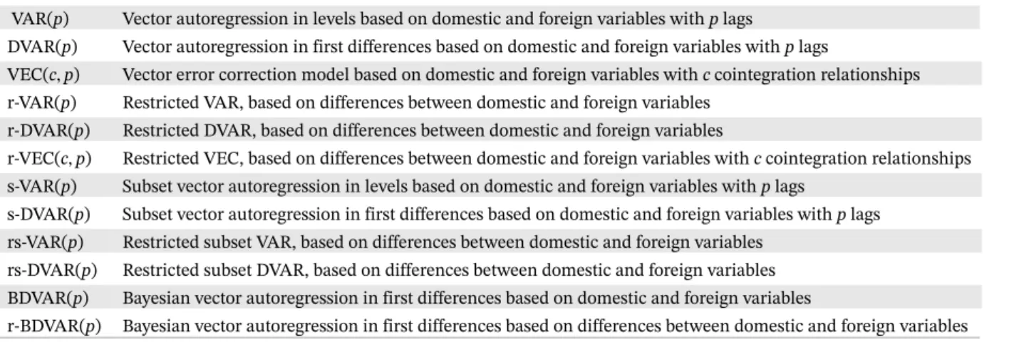
Table 1 lists the 12 individual forecast models used.
2.2 Forecast combinations
The set of methods used to create forecast combinations
from individual multivariate time series models is simi-
lar to that in Costantini et al. (2016). Let S
t𝑗be the spot
TABLE 1 Individual forecast models
VAR(p) Vector autoregression in levels based on domestic and foreign variables withplags
DVAR(p) Vector autoregression in first differences based on domestic and foreign variables withplags
VEC(c,p) Vector error correction model based on domestic and foreign variables withccointegration relationships r-VAR(p) Restricted VAR, based on differences between domestic and foreign variables
r-DVAR(p) Restricted DVAR, based on differences between domestic and foreign variables
r-VEC(c,p) Restricted VEC, based on differences between domestic and foreign variables withccointegration relationships s-VAR(p) Subset vector autoregression in levels based on domestic and foreign variables withplags
s-DVAR(p) Subset vector autoregression in first differences based on domestic and foreign variables withplags rs-VAR(p) Restricted subset VAR, based on differences between domestic and foreign variables
rs-DVAR(p) Restricted subset DVAR, based on differences between domestic and foreign variables BDVAR(p) Bayesian vector autoregression in first differences based on domestic and foreign variables
r-BDVAR(p) Bayesian vector autoregression in first differences based on differences between domestic and foreign variables
exchange rate of euros (EUR) per foreign currency unit (FCU) of currency j, that is, EUR/FCU, at time t, and let S ̂
𝑗m,t+h|tbe the exchange rate forecast of euros per for- eign currency unit of currency j obtained using model m, m = 1 , … , M, for time t + h conditional on the informa- tion available at time t (i.e., h is the forecast horizon). In the following we drop superscript j to keep the exposition simpler. The combinations of forecasts entertained in this study, S ̂
c,t+h|t, take the form of a linear combination of the predictions of individual specifications:
S ̂
c,t+h|t= w
hc,0t+
∑
M m=1w
hc,mtS ̂
m,t+h|t, (6) where c is the combination method, M is the num- ber of individual forecasts and the weights are given by {w
hc,mt}
Mm=0.
Since several combination methods require statistics based on a hold-out sample where the relative predictive ability of models is assessed, let us introduce here some notation on subsample limits: T
0is used to denote the first observation of the available sample, the interval (T
1, T
2) is used as a hold-out sample to obtain weights for those meth- ods where such a subsample is required, and T
3is the last available observation. The sample given by (T
2, T
3) is the proper out-of-sample period used to compare the different methods.
In order to pool the forecasts of individual specifica- tions, we consider a large number of combination methods proposed in the literature. These are the same methods that have been recently used in Costantini et al. (2016) to evaluate exchange rate predictability:
3• Mean, trimmed mean, median. For the mean prediction, w
hmean,0t= 0 and w
hmean,mt=
1M
in Equation 6. The trimmed mean uses w
htrim,0t= 0 and w
htrim,mt= 0 for the individual models that generate the smallest and largest
3Costantini et al. (2016) provide a more detailed discussion of these forecast averaging methods.
forecasts, while w
htrim,mt=
1M−2
for the remaining indi- vidual models. For the median combination method, S ̂
c,t+h|t= median{ S ̂
m,t+h|t}
Mm=1is used (see Costantini &
Pappalardo, 2010).
• Ordinary least squares (OLS) combination. The weights of this method coincide with the estimated coefficients obtained by regressing actual exchange rates on a con- stant and corresponding exchange rate forecast. In our application we use a rolling window over the hold-out sample. Granger and Ramanathan (1984) provide more details on this simple forecast pooling methodology.
• Combination based on principal components (PC). This method allows us to overcome multicollinearity of pre- dictions across models by reducing them to a few prin- cipal components (factors). The method is identical to the OLS combining method by replacing forecasts with their principal components. In our application, we choose the number of principal components using the variance proportion criterion, which selects the small- est number of principal components such that a certain fraction of variance is explained. We set the proportion to 80%.
4• Combination based on the discount mean square forecast errors (DMSFE). Following Stock and Watson (2004), the weights in Equation 6 depend inversely on the historical forecasting performance of individual mod- els, w
hDMSFE,m,t= WMSE
−1mth∕ ∑
Ml=1
WMSE
−1lth, where WMSE
mth= ∑
t̃t=T1+h−1
𝜃
T−h−̃t(
S
̃t− S ̂
m,̃t|̃t−h)
2, for t = T
2− h , … , T
3− h, m = 1 , … , M, w
hDMSFE,0,t= 0, and 𝜃 is a discount factor. In the empirical application, we use 𝜃 = 0 . 95.
• Combination based on hit/success rates (HR). The method uses the proportion of correctly predicted
4More details on the method are provided in Hlouskova and Wagner (2013), where the principal components augmented regressions are used in the context of the empirical analysis of economic growth differentials across countries. Except for Costantini et al. (2016), we are not aware of the existence of any study using this approach in the context of the exchange rate forecasts.
directions of exchange rate changes of model m to the number of all correctly predicted direc- tions of exchange rate changes by the models used, w
hHR,mt= ∑
t̃
t=T1+h−1
DA
m,̃th∕ ∑
M l=1(∑
t𝑗=T1+h−1
DA
l,̃th)
, where t = T
2− h, … , T
3− h and the index of direc- tional accuracy is given by DA
m,th= I (
sgn(S
t− S
t−h)
= sgn ( S ̂
m,t|t−h− S
t−h) )
, where I(·) is the indicator function.
• Combination based on the exponential of hit/success rates (EHR) (Bacchini, Ciammola, Iannaccone,
& Marini, 2010). The weights in this method are w
hEHR,mt= exp (∑
t̃
t=T1+h−1
(DA
m,̃th− 1) )
∕
∑
Ml=1
exp (∑
t̃
t=T1+h−1
(DA
l,̃th− 1) )
, where t = T
2− h , … , T
3− h.
• Combination based on the economic evaluation of directional forecasts (EEDF). The weights in this method capture the ability of models to pre- dict the direction of change of the exchange rate, while taking into account the magnitude of the realized change and are thus given by w
hEEDF,mt=
∑
t̃
t=T1+h−1
DV
m,̃th∕ ∑
M l=1(∑
t̃
t=T1+h−1
DV
l,̃th)
, where
t = T
2− h , … , T
3− h and DV
m,th= | S
t− S
t−h| DA
m,th.
• Combination based on predictive Bayesian model aver- aging (BMA). The weights used are based on the corresponding posterior model probabilities based on out-of-sample (rather than in-sample) fit. See, for example, Raftery, Madigan, and Hoeting (1997), Carriero, Kapetanios, and Marcellino (2009), Crespo Cuaresma (2007), and Feldkircher (2012).
We create weights based on comparing log-predictive scores of the different models in a hold-out subsam- ple, as this prediction error statistic is routinely used in methodological comparisons involving BMA (see, e.g., Fernandez, Ley, & Steel, 2001). The weights are thus given by
w
hBMA,mt=
∑
t̃t=T1+h−1
exp
{
− [
1 2
log
( 2𝜋 ̂𝜎
m,̃2t|̃t−h) +
12
(
S̃t−Ŝm,̃t|̃t−ĥ𝜎m,̃t|̃t−h
)
2]}
∑
M l=1∑
t̃
t=T1+h−1
exp {
− [
1 2
log
(
2 𝜋 ̂𝜎
l2,̃t|̃t−h) +
12
(
S̃ t−Ŝl,̃t|̃t−h
̂𝜎l,̃t|̃t−h
)
2]} , (7)
where ̂𝜎
m2,̃t|̃t−his the estimated variance of the corresponding prediction for model m, S ̂
m,̃t|̃t−h, and t = T
2− h, … , T
3− h.
• Combinations based on frequentist model aver- aging (FMA) (see Claeskens & Hjort, 2008;
2003). The weights are calculated as w
hFMA,mt= exp
(
−
12
IC
mt)
∕ ∑
M l=1exp
(
−
12
IC
lt)
, where IC
mtstands
for an information criterion of model m and t is the last time point of the data over which models are estimated.
We use combinations of forecasts based on the AIC, Schwarz criterion (BIC), and Hannan–Quinn criterion (HQ). The weights corresponding to the BIC can be interpreted as an approximation to the posterior model probabilities in BMA.
5A list of all forecast combination methods we use can be found in Table 6 in the supporting information Appendix.
2.3 Predictive accuracy
Exchange rate forecasts are evaluated using the traditional mean square error (MSE).
6We obtain the standard square error SE
m,t,h= ( S ̂
m,t|t−h− S
t)
2by a rolling-window estima- tion; that is, we keep the estimation sample size constant (equal to T
1− T
0) as we re-estimate the models, thus moving the window that defines the sample used to esti- mate the model parameters. The MSE for each model and forecast combination method is thus calculated over the out-of-sample period for a given forecast horizon h and aggregated as
7MSE
mh= 1∕(T
3− T
2+ 1) ∑
T3−T2𝑗=0
SE
m,T2+𝑗,h.
In addition, we compute composite forecasts based on the MSE of predictions from all models and combination methods over a certain period. In particular, for this tech- nique at each time point t we choose the model or forecast combination method (and thus also the forecast for time point t + h) with the minimum MSE over a certain time window ending at time point t, S ̂
MSE,lt+h|t= S ̂
mMSElth ,t+h|t
, where m
MSElth= arg min
m∑
t𝑗=l
SE
m,𝑗,h. Time point l, such that T
2≤ l ≤ t, defines the beginning of the window over which the performance is evaluated. The evaluation window is [l, t], where l ≤ t ≤ T
3. For our empirical results we use l = t−12;
that is, the model or forecast combination method with the smallest MSE over the last 12 months is chosen.
5See Raftery et al. (1997) and Sala-i-Martin, Doppelhofer, & Miller (2004).
6In a previous version of this paper we also use profit measures such as the directional value, statistics that capture the economic value of directional forecasts and returns with respect to the two trading strategies (see Crespo Cuaresma, Fortin, & Hlouskova, 2017). However, we restrict ourselves to the MSE here.
7The termmodeland thus also its abbreviationmis used in a broader sense that includes both individual models and forecasting rules and methods (like forecast combinations and composite forecasts).
2.4 Trading strategies
We use two trading strategies in order to define the three single assets (three assets for each trading strategy) that the investor can select from. Trading strategy 1 (TS1) is based on buying the foreign currency if its price is forecast to rise and selling it when its price is forecast to fall (“buy low, sell high strategy”), and trading strategy 2 (TS2) exploits the forward rate unbiased expectation hypothesis and is related to the so-called carry trade strategy (“carry trade based strategy”).
Trading strategy 1 is a simple “buy low, sell high” trading strategy as described in Gençay (1998), where the sell- ing/buying signal is based on the current exchange rate.
Forecast upward movements of the exchange rate with respect to the actual value (positive returns) are executed as long positions, while forecast downward movements (negative returns) are executed as short positions. For each exchange rate model and forecast combination method m and forecast horizon h the trading strategy 1 is defined by the following trading signal, 𝑦
𝑗thm,TS1, and (discrete) return, r
t+h𝑗m,TS1,h:
𝑦
𝑗thm,TS1=
{ 1 , if S ̂
𝑗t+h|tm< S
𝑗t(one FCU of currency 𝑗 is sold at t and bought att + h)
−1 , if S ̂
𝑗t+h|tm> S
𝑗t(one FCU of currency 𝑗 is bought at t and sold at t + h), (8)
r
t+h𝑗m,TS1,h=
⎧ ⎪
⎪ ⎨
⎪ ⎪
⎩
1 S𝑗t
( S
𝑗t− S
𝑗t+h
)
= 1 −
S𝑗 t+h
S𝑗t
, if 𝑦
𝑗thm,TS1= 1
1 S𝑗t
(
S
𝑗t+h− S
𝑗t)
=
S𝑗 t+h
St𝑗
− 1, if 𝑦
𝑗m,TS1th= −1,
Trading strategy 2 is based on exploiting the forward rate unbiased expectation hypothesis. In perfect markets, the forward exchange rate is an unbiased predictor of the cor- responding future spot exchange rate. If this hypothesis does not hold, a trading strategy based on exchange rate forecasts may earn positive trading profits. This trading strategy thus depends on whether the exchange rate fore- cast is above or below the forward rate. The trading signal,
𝑦
𝑗m,TS2th, and return, r
t+h𝑗m,TS2,h, are defined as follows:
𝑦
𝑗thm,TS2=
{ 1 , if S ̂
𝑗t+h|tm< F
t+h|t𝑗(one FCU of currency 𝑗 is sold forward at t and bought at t + h)
−1 , if S ̂
𝑗t+h|tm> F
𝑗t+h|t(one FCU of currency 𝑗 is bought forward at t and sold at t + h), (9)
r
𝑗t+h,hm,TS2=
⎧ ⎪
⎨ ⎪
⎩
1 F𝑗t+h|t
(
F
t+h|t𝑗− S
𝑗t+h
)
= 1 −
S𝑗 t+h
Ft+h|t𝑗
, if 𝑦
𝑗thm,TS2= 1
1 F𝑗t+h|t
( S
𝑗t+h
− F
t+h|t𝑗)
=
S𝑗 t+h
F𝑗t+h|t
− 1 , if 𝑦
𝑗thm,TS2= −1 ,
where F
t+h𝑗 |tis the forward exchange rate (EUR/FCU) at time t with respect to currency j, maturing at time t + h.
2.5 Optimal portfolios
In order to assess whether exchange rate forecasts based on macroeconomic fundamentals improve the profitabil- ity of currency portfolios, we investigate the performance of (optimal) currency portfolios of returns implied by two strategies described above, which exploit the potential pre- dictability of exchange rate changes. The optimal portfolio consists of returns implied by a certain trading strategy applied to the three foreign exchange rates EUR/USD, EUR/GBP, and EUR/JPY. We refer to these individ- ual returns as (single) assets based on the EUR/USD, EUR/GBP, and EUR/JPY exchange rates, respectively.
In building optimal portfolios, investors behave accord- ing to particular preferences. We model the following types of preferences: mean–variance (MV), conditional value-at-risk (CVaR), linear, linear loss aversion (LLA), and quadratic loss aversion (QLA). As benchmark portfo- lios, relative to which the optimal portfolios are evaluated,
we consider both (i) the single assets based on individual exchange rates from which the optimal portfolios arecom- posed, as well as (ii) equally weighted (EW) portfolios.
8Consider an investor who dynamically (e.g., on a monthly basis) re-balances her portfolio. Let r
TSth= ( r
USD,TSth, r
GBP,TSth, r
thJPY,TS)
′, where r
thUSD,TSis the return at time t implied by trading strategy TS and exchange rate fore- casts of the EUR/USD for horizon h. Similarly, r
GBP,TSthis the return based on EUR/GBP exchange rate forecasts,
8A portfolio with equal weights was also investigated in Burnside et al.
(2008) and Burnside, Eichenbaum, and Rebelo (2011), using the carry trade strategy (exploiting the forward rate unbiased expectation hypothe- sis) and the momentum strategy (stipulating to sell when it was profitable to sell before).
and r
JPY,TSthis the return based on EUR/JPY exchange rate forecasts. Let x
TSth= (
x
thUSD,TS, x
GBP,TSth, x
thJPY,TS)
′, where x
thi,TSdenotes the proportion of wealth invested at time t in trading strategy TS, whose returns are implied by MSE-based composite forecasts of exchange rate i for hori- zon h. Returns are constructed with respect to composite forecasts based on the traditional MSE. This means that forecasting models (or forecast combination methods) are chosen such that the MSE is the smallest over a span of 12 months, a period that appears to be appropriate in order to capture changing market conditions.
9In our application the returns are available from Jan- uary 2005 until January 2016 at a monthly frequency, and the optimization exercises are performed for a 3-year rolling window; that is, we optimize over 36 observations.
The evaluation period is therefore January 2008 to Jan- uary 2016 (97 observations). The portfolio optimization exercises are carried out under the following preference schemes:
• Mean–variance (MV) preferences. We consider investors that minimize the variance of their portfolio:
min
xTSth
{( x
TSth)
′Σ ̂
TSt+h|tx
TSth| 0 ≤ x
TSth≤ 1 , 1
′x
TSth= 1
} , (10)
where 0 = (0, 0, 0)
′, 1 = (1, 1, 1)
′, and Σ ̂
TSt+h|tis the esti- mate of the (3 × 3)-dimensional conditional covariance matrix of returns implied by the trading strategy TS and model (or forecast combination method or composite forecasts) m.
10• Conditional value-at-risk (CVaR) preferences. We con- sider an investor that maximizes the conditional expec- tation of the left tail of portfolio return distribution such that portfolio returns do not exceed the 𝛽 's quantile of of portfolio return, that is:
(
xmax
TSth,𝛼𝛽) {
E (( x
TSth)
′r
TSth)| ||
| ( x
TSth)
′r
TSth≤ 𝛼
𝛽, 0 ≤ x
TSth≤ 1 , 1
′x
TSth= 1 }
,
(11)
where 𝛽 ∈ (0, 1) and 𝛼
𝛽is the 𝛽-quantile of the portfolio return. Problem 11 is equivalent to
11(
xmax
TSth,𝛼𝛽) {
𝛼
𝛽− 1 t 𝛽
∑
t l=1[ 𝛼
𝛽− ( x
TSth)
′r
TSlh]
+||
|| ||
0 ≤ x
thTS≤ 1 , 1
′x
TSth= 1 } ,
(12)
9In a related analysis using similar returns, we also examined longer and shorter time periods to determine the composite forecast. First we looked at the performance results based on using the total period up to timet, which were usually worse than those based on a period of 12 months.
Then we experimented with a period of 6 months, which in most cases resulted in similar or lower performance measures.
10For a seminal presentation of the mean–variance model, see Markowitz (1952).
11See Rockafellar and Uryasev (2000) for more details.
where [t]
+denotes the maximum of 0 and t. In our application we take 𝛽 = 0 . 05.
• Linear preferences. Investors with linear utility functions maximize the expected return of their portfolio:
max
xTSth
{ E (( x
TSth)
′r
TSth) | || 0 ≤ x
thTS≤ 1 , 1
′x
TSth= 1 } .
(13) We denote this investor the “linear” investor.
• Linear loss aversion (LLA) preferences. Loss aversion, which is a central finding of prospect theory (see Kah- neman & Tversky, 1979) describes the fact that people are more sensitive to losses than to gains, relative to a given reference point ̂𝑦
t. The simplest form of such loss aversion is linear loss aversion, where the marginal util- ity of gains and losses is fixed.
12Linear loss aversion preferences can be modeled as
max
xTSth
{
E (( x
TSth)
′r
TSth− 𝜆 [
̂𝑦
t− ( x
thTS)
′r
TSth]
+)|
|| ||
0 ≤ x
TSth≤ 1 , 1
′x
thTS= 1 } ,
(14)
where 𝜆 > 0 is the loss aversion (or penalty) param- eter. Under the given utility, investors face a trade-off between return on the one hand and shortfall below the reference point on the other hand. Interpreted dif- ferently, the utility function contains an asymmetric or downside risk measure, where losses are weighted dif- ferently from gains. In our application we take the zero return as the reference point; that is, ̂𝑦
t= 0, and 𝜆 = 1 . 25 , 5.
• Quadratic loss aversion (QLA) preferences. Under quadratic loss aversion preferences, large losses are punished more severely than under linear loss aversion preferences.
13The quadratic loss aversion preferences can be modeled as
max
xTSth
{ E
( ( x
TSth)
′r
TSth− 𝜆 ([
̂𝑦
t− ( x
TSth)
′r
TSth]
+)
2)|
|| ||
| 0 ≤ x
TSth≤ 1 , 1
′x
TSth= 1 }
,
(15) where the notation is the same as in the LLA pref- erences; that is, in our application we take again the zero return as the reference point, ̂𝑦
t= 0, and 𝜆 = 1 . 25 , 5. The problems given by Equations 14 and 15 are equivalent to higher-dimensional linear programming problems (see Fortin & Hlouskova, 2015).
12The optimal ass et allocation decision under linear loss aversion has been extensively studied; see, for example, Gomes (2005), He and Zhou (2011), and Fortin and Hlouskova (2011).
13The penalty on losses under quadratic loss aversion is also referred to as quadratic shortfall.
2.6 Performance
2.6.1 Performance measures
The main performance measures we consider are the mean return, the Omega measure, the Sharpe ratio (SR) and the Sortino ratio (SoR), where the last three mea- sures are risk adjusted and in that sense reflect better the overall considerations of a typical investor (who is not only interested in the portfolio return but also in the portfolio risk). These measures are, among others, reported in our empirical results. The Omega measure is the upside potential of the return with respect to its downside potential relative to the zero return, Omega =
∑
ni=1
| max{r
i, 0} | ∕ ∑
ni=1
| min{r
i, 0} | , where i = 1 corre- sponds to January 2008 and i = n to January 2016. A larger ratio indicates that the asset provides the chance of more gains relative to losses. The Omega measure is a risk-adjusted performance measure which considers all moments of the return distribution, whereas the Sharpe and Sortino ratios only consider the first two moments (a modified version of the second moment in the case of the Sortino ratio).
14The Sharpe ratio is the mean divided by the volatility of the return, the Sortino ratio is a modified version of the Sharpe ratio which uses downside volatility with respect to the zero return (instead of standard devia- tion) as the denominator, i.e., SR = r∕𝜎 ̄ and SoR = r∕𝜎 ̄
D, where r ̄ and 𝜎 are the mean and the standard deviation of r
tcalculated with respect to the sample January 2008 through January 2016, and 𝜎
Dis the downside volatil- ity (with respect to the zero return) calculated as 𝜎
D=
√
1 n∑
ni=1
(min{r
i, 0})
2, where i = 1 corresponds to January 2008 and i = n to January 2016.
15The natural bench- mark return for our application appears to be a zero return, reflecting that the investor does not take any position in the foreign exchange market. In both cases a larger ratio indicates a higher return per unit of risk, so usually higher figures denote a better performance. This does not apply, however, when the mean return is negative.
2.6.2 Bootstrap test for equal performance
In order to assess whether the performance superiority of certain (optimal) portfolios is systematic and not due to luck, we perform the bootstrap stepwise multiple superior
14The formal definition of the Omega measure is ∫
∞ tr(1−F(x))dx
∫−∞tr F(x)dx = E(X−tr|X>tr)P(X>tr)
E(tr−X|X≤tr)P(X≤tr), where F(·)is the cumulative distribution function of returns andtris the target return, which in our case is zero.
15In our empirical results we also present a performance measure labeled “downside volatility ratio” that gives the proportion of down- side volatility to the downside and upside volatility𝜎U, where𝜎U =
√1 n
∑n
i=1(max{ri,0})2, and thus the ratio is calculated as 𝜎D
𝜎D+𝜎U
.
predictive ability test (stepM-SPA) by Hsu, Hsu, and Kuan (2010) for the comparison of optimal portfolio perfor- mance with respect to the benchmark models. The test is based on the bootstrap method of Politis and Romano (1994), the stepwise test of multiple check by Romano and Wolf (2005) and the test for superior predictive ability of Hansen (2005).
16The following relative performance measures, d
TSopt,th, opt = MV, CVaR, linear, LLA, and QLA with 𝜆 = 1 . 25 , 5, t = January 2008 to January 2016, h = 1, 3, 6, 12, are com- puted and the tests are defined based alternatively on d
TSopt,th= r
TSopt,th− r
TSB,thand d
TSopt,th= Omega
TSopt,th− Omega
TSB,th. As benchmark portfolios, for which the corresponding measures (denoted by subindex B) are calculated, we con- sider the single assets based on the returns implied by a certain trading strategy which is applied to single exchange rates, as well as the equally weighted portfolio (EW). The single assets and the equally weighted portfolio are either based on composite forecasts or on the random walk. Note that the performance measure related to Omega is defined as Omega
t= max{r
t, 0}∕(
1n
∑
ni=1
| min{r
i, 0}|), where we skip indices and superscripts to simplify the notation. Note that the bootstrap test cannot be performed for the Sharpe and the Sortino ratios, as for negative values it is not true that larger values are associated with a better performance (the test involves the ordering of calculated statistics).
17The bootstrap stepM-SPA test is a comprehensive test across all portfolio optimization models under consider- ation and directly quantifies the effect of data snooping by testing the null hypothesis that the performance of the best model is no better than the performance of the bench- mark model. For the seven optimization models opt =MV, CVaR, linear, LLA with 𝜆 = 1 . 25 , 5, and QLA with 𝜆 = 1.25, 5; we consider the test of H
opt0∶ E ( d
TSopt,th≤ 0
)
against H
Aopt∶ E ( d
TSopt,th> 0 )
. In our empirical application we use the output of the test to identify those optimal port- folios that outperform the benchmark portfolio at a certain significance level.
2.6.3 Break-even transaction costs
The break-even transaction cost, 𝜏
be, is that constant (pro- portional) transaction cost that makes the net gain (net of transaction cost) of the optimal portfolio equal to the net gain of the benchmark portfolio
18:
16For more details on the test, see Hsu et al. (2010).
17For example, with a higher volatility the Sharpe ratioincreasesinstead ofdecreases, given that the mean is negative.
18Break-even transaction costs are also considered in Han (2006), Della Corte et al. (2009), and Della Corte and Tsiakas (2013), for example. Our computations are based on the transaction value (over the total period of the investment strategy) whereas their computations are based on (one-period) returns.
𝜏
be=
∑
T t=2(
V
topt− V
t−1opt)
− ∑
T t=2( V
tB− V
t−1B)
∑
Tt=2
V
topt∑
n i=1|| ||
| x
opti,t−
xopt i,t−1
( 1+riopt,t ) 1+ropt𝑝,t
|| ||
| − ∑
Tt=2
V
tB∑
m i=1|| ||
| x
Bi,t−
xB i,t−1
( 1+rBi,t) 1+rB𝑝,t
|| ||
|
(16)
where V
tis the value of the (optimal/benchmark) portfo- lio at time t, x
i,tis the weight of asset i at time t in the (optimal/benchmark) portfolio, r
i,tis the return of asset i at time t in the (optimal/benchmark) portfolio, and r
p,tis the return of the (optimal/benchmark) portfolio at time t.
Superscripts opt and B denote the optimal and the bench- mark portfolios, respectively. We assume that the initial investment in both portfolios is the same; that is, V
1opt= V
1B.
19We compare all optimal portfolios (MV, CVaR, linear,
LLA
𝜆=1.25, LLA
𝜆=5, QLA
𝜆=1.25, and QLA
𝜆=5) with the three
single assets and the EW portfolio, based on composite forecasts and on the random walk, respectively.
If the actual transaction cost is lower than the break-even transaction cost then the optimal portfolio achieves a larger gain than the benchmark portfolio, after controlling for transaction costs.
20So larger break-even transaction costs indicate that the optimal portfolio out- performs the benchmark portfolio more easily, while negative break-even transaction costs suggest that the optimal portfolio does not outperform the benchmark portfolio. For the discussion of our empirical results we use a value of 0.1% for the actual transaction cost.
213 E M P I R I C A L R E S U LT S
3.1 Data, estimation, and predictions
We base our empirical analysis on monthly data span- ning the period from January 1980 until January 2016 for the EUR/USD, EUR/GBP, and EUR/JPY exchange rates.
The beginning of the sample is thus T
0= January 1980;
the beginning of the hold-out forecasting sample for indi- vidual models used in order to obtain weights based on predictive accuracy is given by T
1= January 2000. The
19The break-even transaction cost is not sensitive with respect to the starting value.
20In fact this is only true if the trading cost for the optimal portfolio is larger than the trading cost for the benchmark portfolio (i.e., if the denominator in Equation 16 is positive), which is always true in our appli- cations. Note that it is often a typical feature of the benchmark portfolio that the involved amount of trading is rather small.
21Marquering and Verbeek (2004), for example, consider three levels of transaction costs, 0.1%, 0.5%, and 1%, to represent low, medium, and high costs. They consider equity and bond transactions, however, while we consider currency transactions. The latter usually involve lower trans- action costs. For example, the average bid–ask spread related to the middle price over our sample period ranges from 0.02% for the EUR/USD exchange rate to 0.06% for the EUR/JPY exchange rate. So a transaction cost of 0.1% seems to be a quite high level in the foreign exchange market.
beginning of the actual out-of-sample forecasting sample is T
2= January 2005, and the end of the data sample is T
3= January 2016. All data are obtained from Thomson Reuters Datastream.
22Given the large set of statistics computed for the analy- sis, we start by describing how the results are depicted in the tables. We first report results on the performance of optimal currency portfolios constructed by different types of investors, namely MV, CVaR, linear, linear loss averse
(LLA
𝜆=1.25, LLA
𝜆=5), and quadratic loss averse (QLA
𝜆=1.25,
QLA
𝜆=5) investors (the first seven data columns in the tables of results). The optimal portfolios consist of three single assets, the returns of which are implied by a certain trading strategy (from the two trading strategies described above) with respect to MSE-based composite forecasts of the EUR against the USD, GBP, and JPY. In addition, we present results on how these optimal portfolios compare to benchmark portfolios, which include the three single assets that compose the portfolio as well as the equally weighted portfolio (the following four data columns in the tables of results). We also consider as benchmark portfolios the three single assets which are based on the simple random walk (RW) model to forecast exchange rates (instead of on composite forecasts) as well as the equally weighted portfolio of these three assets (the last four data columns).
The tables are structured in five horizontal blocks. The first block presents the four main performance measures on which we base our analysis: the mean return, the Omega measure, the Sharpe ratio, and the Sortino ratio.
For two of them, the mean and the Omega measure, we also performed the bootstrap-based stepM-SPA test of Hsu et al. (2010). The second block shows additional statistical descriptives, namely median, volatility, downside volatil- ity, downside volatility ratio, CVaR, skewness, and kurto- sis. The third block presents break-even transaction costs for the optimal portfolios, first in relation to the bench- mark portfolios based on composite forecasts (where the evaluation criterion is the MSE over the last 12 months) and then in relation to the benchmark portfolios based on the random walk. For the discussion of our empirical results we use a value of 0.1% for the actual transaction cost. The fourth block shows the realized returns over the last 5, 3, and 1 years, and the last block gives the mean portfolio allocations.
22Details on the sources for all variables used are given in the Appendix.
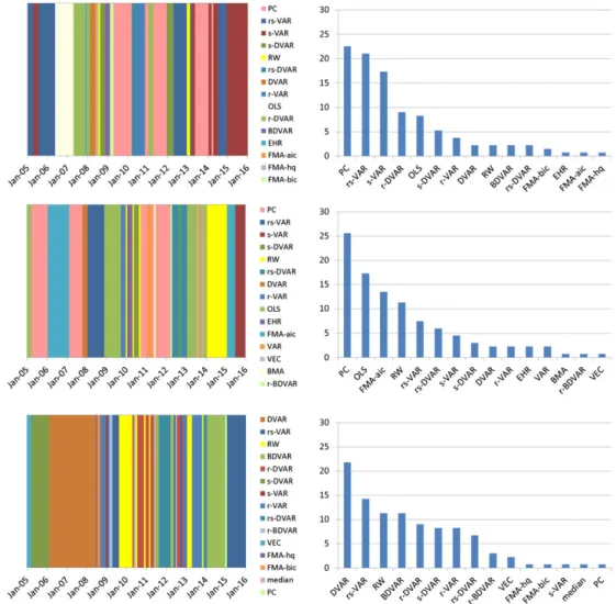
FIGURE 1 MSE-based best forecast models for 1-month-ahead forecasts. The figure shows the best forecast models, that is, the models generating the composite forecasts (left) and the distribution of the best models, that is, the number of times different forecast models are selected over the total period, in percent (right). From top to bottom the figure presents best models for the EUR/USD, the EUR/GBP, and the EUR/JPY [Colour figure can be viewed at wileyonlinelibrary.com]