Computational Materials Science

(1)

Computational Materials Science

Prof. Karsten Held

Institut f¨ ur Festk¨orperphysik, TU Wien

October 15, 2009

(2)

(3)

Chapter 1 Introduction

1.1 Materials Hamiltonian

In contrast to particle physics, we know in solid state theory our ‘theory of every- thing’, i.e., for every material. At the energy range we are interested in, i.e., between µeV’s and keV’s, only the Coulomb interaction (and the kinetic energy) plays a role.

That is, we can disregard gravitation, strong, and electroweak interactions. If we take into account the mutual Coulomb interaction between our constituents, the nuclei (nuc) and electrons (el) of the given material ¹, we arrive at the following Hamiltonian

H = Hnuc+Hel+Hel−nuc , (1.1)

where, as an input, we only have the charge of the nuclei Ze, their mass M, the charge of the electron−e, and their massm. We will in general assume that relativis- tic effects are not important, and retardation effects can be neglected. Therefore, the different parts of the Hamiltonian above can be written quite generally as follows

Hnuc =

XN

i

P²_i 2Mi

+1 2

X

i6=j

e²ZiZj

|R_i−R_j | , (1.2)

Hel =

ZNX

i

p²_i 2m +1

2

X

i6=j

e²

|r_i−r_j | , (1.3)

Hel−nuc = −^X

i,j

e²Zj

|r_i−R_j | . (1.4)

Here, R_i denotes the position operator of the N nuclei, P_i = ¯h/i ∂/∂Ri their momentum operator; r_i and p_i = ¯h/i ∂/∂r_i are position and momentum operator for the ZN electrons.

While we know the solid state Hamiltonian (1.1), we cannot solve it: Not an- alytically for more than two particles, and even not numerically for more than a

1We could also add the inner shell electrons to the nuclei so that we deal with ions and outer electrons instead.

5

(6)

very few [O(10)]. This is because of the Coulomb interaction, which correlates the movement of all electrons and nuclei, so that we have to solve a quantum mechanical many-body problem. For such a problem, the numerical effort grows exponentially with the number of particles, and such an exponential problem cannot be solved for significantly many particles, even if computer power continued to grow rapidly.

Note that for a macroscopic piece of matter, of say 1 cm³, we have N ∼ O(10²³) nuclei. While this clearly shows that a numerical solution of the solid state Hamil- tonian (1.1) is impossible, it also means that we can consider the thermodynamic limit N → ∞. This allows us to use (quantum) statistical mechanics, which is a tremendous simplification compared to a mesoscopic system of say N ∼ O(1000) nuclei.

Nonetheless, we have to develop approximations and we start with the first one in the next section.

1.2 Born-Oppenheimer approximation

Let us make use of the fact that the movement of the electrons is much faster than that of the nuclei because of their lighter massm/M ∼10⁻³−10⁻⁴, as the the mass of a single nucleon is approximately 1.800 times larger than that of the electron.

This implies that

E_nuc^kin.

E_el^kin. ≪1, (1.5)

where by E^kin. we denote the kinetic energy of nuclei and electrons, respectively.

This means physically: Since the electrons are much faster than the nuclei, they will be able to accommodate instantaneously to the position of the nuclei, on the time scale that characterizes the motion of the latter.

These are the conditions suitable for the adiabatic approximation. We are not going to give the proof of the adiabatic theorem (see e.g. A. Messiah Quantum mechanics, Vol. 2 Sec. 17.2.4 - 17.2.7), but merely use it. Preconditions for the adiabatic theorem is a time dependent Hamiltonian H(t) which

i) changes infinitely slowly (adiabatically) and

ii) for every t the eigenvalues ofH(t) are non-degenerate, i.e., ǫj(t)6=ǫk(t) for all t and all j 6=k.

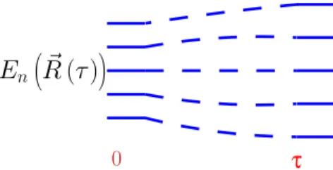
Then, our system always stays in the same eigenvalue j when evolving in time, see Fig. 1.1. This implies that we only need to consider the instantaneous eigenvalues and eigenvectors of H(t) for allt.

In the case of the solid state Hamiltonian (1.1), the position of the nuclei is a function of time R_i = R_i(t), changing slowly (adiabatically) in comparison to

(7)

K . Held - Computational Materials Science 7

E

n 0

~

R() 1

A

0 τ

Figure 1.1: Schematic evolution (fromt= 0 toτ) of the eigenvalues in the adiabatic limit .

the fast movement of the electrons. In the adiabatic approximation, called Born- Oppenheimer approximation in our case of nuclei and electrons, we can hence consider the instantaneous Hamiltonian for the electrons

Hel+Hel−nuc =

XZN

i

−¯h² 2m

∂²

∂r²_i −^X

i,j

e²Zj

|r_i−R_j | +1 2

X

i6=j

e²

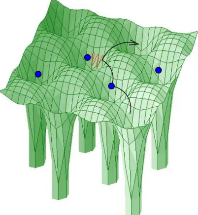
|r_i−r_j | (1.6) with fixed nuclei position at every time t, see Fig. 1.2 for an illustration.

For fixed time, i.e., fixed R, we need to solve a Schr¨odinger equation for the electrons

(Hel+Hel−nuc)ψj(r,R) = E_j^el(R)ψj(r,R) , (1.7) with

r = (r1, . . . ,r_ZN) ,

R = (R1, . . . ,R_N) , (1.8) R giving the instantaneous positions of the nuclei. Figure 1.1 gives a sketch of the evolution of the eigenvalues for the electrons.

Since we stay in the same eigenstate for the electrons, e.g., the ground state ψ0, we can now obtain the eigenfunction for the whole Hamiltonian (1.1) through the product ansatz

Ψ (r,R) = ψ0(r,R) Φ (R) . (1.9)

Then

H =

XN

i

P²_i 2Mi

+ 1 2

X

i6=j

e²ZiZj

|Ri−Rj |+Hel+Hel−nuc (1.10)

applied on Ψ gives HΨ = −

XN

i

¯ h² 2Mi

∂²

∂R²_iΨ + 1 2

X

i6=j

e²ZiZj

|Ri−Rj |

| {z }

U0(R)

Ψ +E₀^el(R) Ψ

(8)

Figure 1.2: Within the Born-Oppenheimer approximation, the electrons move (arrow) in the static lattice potential of the ions (green) and interact with the other electrons through the Coulomb interaction (red). Due to the latter, the moving electron is repelled by the electron located on the next site. It is energetically favorable if the depicted electron hops somewhere else, as indicated by the arrow. Hence, the movement of every electron is correlated with that of every other.

= ψ0(r,R)

(

−

XN

i

¯ h² 2Mi

∂²

∂R²_i +E0^el+U0(R)

)

Φ (R)

−

XN

i

¯ h² 2Mi

(

2 ∂Φ

∂Ri

∂ψ0

∂Ri

+ Φ∂²ψ0

∂R²_i

)

| {z }

non-adiabatic part

. (1.11)

Let us first notice, that if we multiply this equation by ψ0^∗(r,R) and integrate over r, the first line above gives us an effective Schr¨odinger equation for the nuclei. After this, we consider the non-adiabatic terms. For the first one we have

Z

d³x ψ^∗0

∂ψ0

∂Ri

= 1

2

∂

∂Ri

Z

d³x ψ0^∗ψ0 = 0 , (1.12) where we used the fact that without magnetic fieldsH =H^∗ so that the wavefunction can be chosen real, and that the total number of electrons cannot be changed by lattice vibrations.

(9)

K . Held - Computational Materials Science 9 For the second non-adiabatic contribution, we assume the worst case that the electrons are tightly bound to the nuclei, i.e., r_i ≈ R_j for some i and j. Then a crude estimate² gives

− ¯h² 2M

XN

j=1

Z

d³x ψ0^∗

∂²ψ0

∂R²_j ≈ − h¯² 2M

XN

i=1

Z

d³x ψ0^∗

∂²ψ0

∂r²_i = m

ME_el^kin. << |E0^el| (1.13) Neglecting the two non-adiabatic terms, the lattice dynamics (phonons) is described by the following Schr¨odinger equation:

"_N X

i

P²_i 2Mi

+E0^el(R) +U0(R)

#

Φ (R) = EΦ (R) . (1.14) The determination of the potential

U(R)≡E0^el(R) +U0(R) (1.15)

is still a rather demanding task. On the one hand, we should be able to deal with the long-range Coulomb potential in U0(R), but on the other hand, we know (we will see this in detail later) that the long-range part will be screened by the electrons. Furthermore, although it is nowadays possible to calculate at least the ground state for the electrons given the positions of the atoms in the frame of the density functional theory.³

At the end of this section, let us note that the most important corrections to the Born-Oppenheimer approximation is not the non-adiabatic term of Eq. (1.11), but stem from the incompleteness of the product ansatz Eq. (1.9). A full ansatz requires to take into account all eigenstatesj:

Ψ (r,R) = ^X

j

ψj(r,R) Φ (R) . (1.16) Then, for a non-infinitely-slow change of the atomic positions, we will have transitions between different eigenstates, given by terms of the form

Z

d³x ψ_j^∗ 1

∂Ri

ψj^′. (1.17)

These terms can be estimated to be ∼^qm/M and are the leading correction to the adiabatic (Born-Oppenheimer) approximation. This is the electron-phonon coupling, describing how the moving nuclei ( ¹

∂Rⁱ) lead to transitions between electronic states (j and j^′).

In practice, the Born-Oppenheimer approximation is a reliable approximation allowing us to describe the lattice degrees of freedom [Eq. (1.6)]. separately from the electronic degrees of freedom [Eq. (1.6)] (with the electron-phonon coupling being the leading correction).

2In a more detailed analysis, using the fact that the lattice vibrations around the equilibrium position areδR²∼1/√

M, one can show that this term is even a factorp

m/M smaller.

3Despite of the approximations involved, this works surprisingly accurately. But the determination of E0^el is even within that approximation rather demanding if it has to be carried out for many nuclei positionsRi.

(10)

1.3 Crystal lattices

We will concentrate here on perfect crystals, i.e. on arrays of atoms, where a given arrangement is repeated forming a periodic structure, in principle over the whole space. Although crystals have in reality a finite extension, they posses of the order of 10²³ atoms, such that to consider them infinite is a rather good approximation.

In doing so, we will disregard those phenomena taking place close to the surface of the crystals. Another emerging field are nanostructures where man-made structures interrupt the crystal periodicity and which will be discussed later.

A restriction due to the assumption of a periodic structure is that we will not consider the effect of impurities and disorder. Impurities can be considered as a perturbation of an ordered system, and as such, their treatment can be seen as an extension of the lectures here. Disorder on the other hand, an important area of research in statistical as well as in solid state physics, prompted the development of many new theoretical techniques like e.g. supersymmetry, needed to study phenomena like localizationorglassy behavior. Unfortunately, we are not going to have time to deal with such interesting subjects.

Once we stated what we are not going to deal with, let us come back to our subject: crystal lattices. Let us start by defining aBravais lattice: Ad-dimensional Bravais lattice consists of all position vectors

R_i =

Xd

j=1

nija_j (1.18)

with integer-numbersnij and basis vectors ai, i= 1, . . . , d.

The simplest crystal lattice is the primitive latticewhere we have the same kind of nuclei on every lattice point R_i of a Bravais lattice. This primitive lattice is invariant under translation symmetry since shifting (translating) a Bravais lattice by any Bravais lattice vector R_i results in the same (infinite) lattice.

We can define the translations through an operator, which act on a function f, e.g., the wave function, by replacing r → r+Ri:⁴

TRⁱ : f(r)→f(r+Ri). (1.19) More complex crystal structures, are described by a lattice with basis where j different nuclei are located at basis vectors r_j relative to the sites of the Bravais lattice, i.e., at R_i +r_j. This lattice has again the translation symmetry defined by the vectors of the Bravais lattice, i.e., it is invariant under all translation by Bravais lattice vectorsR_i. For example, the diamond lattice and all lattices involving different nuclei are lattices with basis.

For describing the whole space which is periodically repeated, we introduce the concept of an elementary cell. This is defined by the smallest volume of space which, when tranlated by all vectors of a Bravais lattice, fills all of space without

4With this standard definition a structure is shifted from zero to −Ri. Consider, e.g., a δ(r) peak which is translated to δ(r+Ri), i.e., the peak shifted from zero to r=−Ri.

(11)

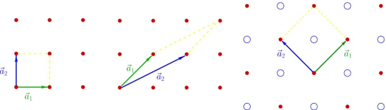
K . Held - Computational Materials Science 11 overlapping. A way to construct the elementary cell is through the parallel-epiped spanned by the basis vectors of the Bravais lattice, see Fig. 1.3. Since these basis vectors are not unique, even this particular construction leads to different choices of the elementary cell.

~a

2

~a

1

~a

1

~a

2

~a

2

~a

1

Figure 1.3: Examples of different elementary cells, i.e., for the same primitive lattice (left and middle) and for a lattice with basis (right).

For obtaining a unique elementary cell, we define the Wigner-Seitz cell as the region of space closer to a point of the Bravais lattice than to any other point.

We can construct constructing the Wigner-Seitz cell, by drawing the perpendicular bisector planes of the translation vectors from one lattice point to its neighbors (Fig.

1.4).

Figure 1.4: Wigner-Seitz cell.

1.4 The reciprocal lattice

Let us suppose for definiteness, that we are dealing with three dimensions, i.e.d= 3.

Then, the volume of the elementary cell is

Ω = a1·(a2×a3) . (1.20)

(12)

Let us define now three new vectors as follows b1 = (2π/Ω)a2×a3

b2 = (2π/Ω)a3×a1

b3 = (2π/Ω)a1×a2











b^α_i = 2π

Ωεijkε^αβγa^β_ja^γ_k

( i, j, k = 1,2,3 α, β, γ = x, y, z(1.21)

εijk andε^αβγ are called Levi-Civita symbols. They are totally antisymmetric tensors with the property

εijk =







1 fori= 1, j = 2, k = 3 or an even permutation of them

−1 fori, j, k an odd permutation of 123 0 for any two indices equal

(1.22) Using the definition of the vectorsb_i and the properties of the Levi-Civita symbols, it can be shown that

a_i·b_j = 2π δij , (1.23)

where δij is called the Kronecker delta with the property δij =

( 1 fori=j

0 else (1.24)

The vectors b_i can be seen as basis vectors of the reciprocal lattice, i.e. they can be used to construct another Bravais lattices with vectors ⁵

G =

X3

j=1

kjb_j , (1.25)

with kj integer. These vectors are called reciprocal lattice vectors. Recalling (1.18), we find an important property of the reciprocal lattice vectors

G·R = ^X

i,j

nikja_i·b_j

= 2π^X

i

niki = 2πM , (1.26)

with M some integer. This implies that

exp (iG·R) = 1, (1.27)

a fact with important consequences for the next point.

Since the reciprocal lattice vectors form a Bravais lattice, we can construct a Wigner-Seitz cell on this lattice. It is called the Brillouin-zone. Its volume can be obtained in the same way as in real space, namely

ΩB =b1·(b2×b3) . (1.28)

Using (1.21), it can be shown that

ΩB = (2π)³

Ω . (1.29)

5dropping the indexiwe had in Eq. (1.18) in the following.

(13)

1.5 Bloch’s theorem.

We consider in this chapter non-interacting electrons under the influence of a static, periodic potential V (r), i.e. such that it fulfills V (r) = V (r+R), where R is a lattice vector.

In this situation, Bloch’s theorem states that the one-particle states can be chosen so that

ψ(r+R) = exp (ik·R) ψ(r) , (1.30) i.e. ψ(r) is a periodic function up to a phase.

Proof

Let R be a lattice vector and TR be a translation operator that acts as follows on any given function

TRf(r) = f(r+R) . (1.31)

By assumption, the Hamiltonian is translational invariant under translations by a lattice vector. It follows that

TRH(r) ψ(r) = H(r+R) ψ(r+R)

= H(r) ψ(r+R) = H(r) TRψ(r) ∀ψ , ∀R.(1.32) This means that

hTR, Hⁱ= 0 ∀R. (1.33)

Since H and the translation operators commute for all translations R, there is a common set of eigenfunctions for H and the set ⁿTR

o of all translation operators of the lattice. Therefore, the one-particle states of the system obey an eigenvalue equation for the translation operators

ψ(r+R) = TRψ(r)

= c(R) ψ(r) . (1.34)

Furthermore, TR is unitary since

TRTR^′ =TR⁺R^′ =⇒c(R+R^′) = c(R^′) c(R) . (1.36) This is easily fulfilled by

c(R) = exp (ik·R) , (1.37)

(14)

for some wavevector k. SinceG·R= 2πn, with n integer, we can restrict k to the first Brillouin zone. Such a form also satisfies eq. (1.36), for any lattice translation vector.

An alternative formulation of Bloch’s theorem is that the wave functions can be chosen such that

ψ(r) = uk(r) exp (ik·r) , (1.38) whereuk(r) is a periodic function with the periodicity of the lattice, andkbelongs to the Brillouin zone. Eq. (1.38) directly implies our first formulation of Bloch’s theorem, i.e., Eq. (1.30). On the other if Eq. (1.30) holds, we can define a function uk(r) = exp (−ik·r) ψ(r) . (1.39) After a translation and applying Eq. (1.30) we have

uk(r+R) = exp (−ik·r) exp (−ik·R) ψ(r+R)

= exp (−ik·r) ψ(r) = uk(r) , (1.40) i.e. uk(r) is a periodic function with the periodicity of the lattice. This means that Eq. (1.38) holds. That is we have shown the equivalence of the two formulations.

Since k is a good quantum number, we can from now on label the wavefunction by k:

ψ(r)−→ψk(r) . (1.41)

1.6 Consequences of Bloch’s theorem: Bandstruc- ture

The first direct consequence of Bloch’s theorem is that the electronic density n(r) = ψ^∗(r)ψ(r) =u^∗k(r)uk(r) (1.42) is a periodic function with the periodicity of the lattice because it was demonstrated above thatuk(r) has this periodicity. Although this was expected, it is comforting to see that this is obtained on purely theoretical grounds, where the only assumption is that the Hamiltonian is periodic.

Since we are dealing with non-interacting electrons under the influence of a periodic potential, the Schr¨odinger equation looks as follows

"

−¯h²

2m∇²+V (r)

#

exp (ik·r) u_n,k(r) =En(k) exp (ik·r) u_n,k(r) , (1.43) that is, u_n,k itself is a solution of a Schr¨odinger equation,

"

¯ h²

2m(−i∇+k)²+V (r)

#

u_n,k(r) =En(k) u_n,k(r) , (1.44)

(15)

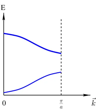
K . Held - Computational Materials Science 15 The subindex n was introduced, since as we know already from a simple problem in quantum mechanics, like the particle in a box, more than one solution of Schr¨odinger’s equation can be found for a given wavevector k. The subindex n denotes the bands in the solid. The set of eigenvalues En(k) is called usually the band-structure.

E

0

a

~

k

Figure 1.5: Sketch of a band-structure.

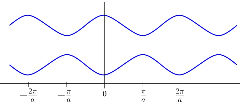
As already discussed in (1.37), we restricted k to the first Brillouin zone, since for any translation, the eigenvalue remains unchanged by an addition of a reciprocal lattice vector. Since this eigenfunction of the translation operator is at the same time an eigenfunction of the Hamiltonian, the eigenenergies are also insensitive with respect to a translation by a reciprocal lattice vector. Therefore, we have

En(k+G) =En(k) . (1.45)

This means that we can consider the energy bands in the first Brillouin zone (re-

(16)

stricted zone scheme - Fig. 1.6) or beyond it (repeated zone scheme - Fig. 1.7).

0

a

Figure 1.6: One dimensional band structure in the reduced zone scheme.

0

a

2

a

a 2

a

Figure 1.7: One dimensional band structure in the repeated zone scheme.

(17)

Chapter 2 Density functional theory (DFT)

The basic idea of density functional theory (DFT) is to work with a simple quantity, i.e. the electron densityρ(r), instead of trying to solve theab initioHamiltonian (1.7) through complicated many-body wave functions. This is possible, at least for the ground state energy and its derivatives, thanks to the Hohenberg-Kohn [1] theorem, which states that the ground state energy is a functional of the electron density E[ρ(r)] which is minimised at the ground state density ρ(r) = ρ0(r). Following Levy [3], this theorem can be easily proven and the functional even be constructed by a two-step minimisation process, see Fig. 2.1. In a first step, we select all many- body wave functions Ψ(r1σ1, ...rNσN) for a fixed number of electronsN which yield a certain electron density ρ(r), and minimise the energy expectation value for these wave functions

E[ρ] = minⁿhΨ|Hˆ|Ψi hΨ|

XN

i=1

δ(r−r_i)|Ψi=ρ(r)^o. (2.1) This is exactly the DFT functional for the ground state energy: A second minimisation yields the ground state energy E0 = minρE[ρ] at the ground state density ρ0, since for the ground state density E[ρ0] includes the energy expectation value w.r.t the ground state wave function, see Fig. 2.1 for an illustration.

While this construction proves the Hohenberg-Kohn theorem, we did actually not gain anything: For obtaining E[ρ] we have to calculate the expectation value hΨ|Hˆ|Ψi for complicated many-body wave functions Ψ. Only the ionic potential Eion[ρ] = ^R d³r Vion(r) ρ(r) and the Hartree term EHartree[ρ] = ¹₂^R d³r^′d³r Vee(r− r^′) ρ(r^′)ρ(r) can be expressed easily through the electron density. Denoting by Ekin[ρ] the kinetic energy functional, we can hence write

E[ρ] =Ekin[ρ] +Eion[ρ] +EHartree[ρ] +Exc[ρ], (2.2) where all the difficulty is now hidden in the exchange and correlation term Exc[ρ].

This term is unknown. An important aspect of DFT is however that the functional E[ρ]− Eion[ρ] does not depend on the material investigated; for a prove see e.g.

[2]. Hence, if we knew the DFT functional for one material, we could calculate all materials by simply addingEion[ρ].

17

(18)

all wave functions

wave functions with wave functions with ρ

ρ

1

2

Figure 2.1: Construction of the DFT functional according to Levy [3]. The DFT energy functional for a given electron density ρ1(r) is the minimal expectation value of all wave functions yielding ρ1(r).

For calculating the ground state energy and density, we have to minimiseδ{E[ρ]− µ(^Rd³rρ(r)− N)}/δρ(r) = 0 where the Lagrange parameter µ fixes the number of electrons to N. To avoid the difficulty of expressing the kinetic energy Ekin[ρ]

through ρ(r), Kohn and Sham [4] introduced an (at this point auxiliary) set of one-particle wave functions ϕi yielding the density

ρ(r) =

XN

i=1

|ϕi(r)|², (2.3)

and minimised w.r.t. the ϕi’s instead of ρ(r). That is, we minimise δ{E[ρ] − εi[^R d³r|ϕi(r)|²]−1}/δϕ^∗_i(r) = 0 where the Lagrange parameters εi guarantee the normalisation of the ϕi’s. This minimisation leads us to the Kohn-Sham [4] equations

"

− ¯h² 2me

∆ +Vion(r) +

Z

d³r^′ Vee(r−r^′)ρ(r^′) + δExc[ρ]

δρ(r)

#

ϕi(r) =εi ϕi(r). (2.4) These Kohn-Sham equations are Schr¨odinger equations, describing single electrons moving in a time-averaged potential

Veff(r) = Vion(r) +

Z

d³r^′ Vee(r−r^′)ρ(r^′) + δExc[ρ]

δρ(r) (2.5)

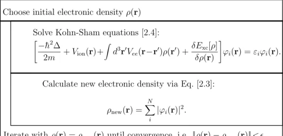
of all electrons. The Kohn-Sham equations and the electron density have to be calculated self-consistently, see the flow diagram Fig. 2.3.

Let us note that the one-particle Kohn-Sham equations serve, in principle, only the purpose of minimising the DFT energy, and have no physical meaning. If we knew the exact Exc, which is non-local in ρ(r), we would obtain the exact ground state energy and density. However, in practise, one has to make approximations to Exc such as the local density approximation discussed in the next Section. We can then think of these approximations as describing single electrons moving in an approximated potential δExc[ρ]/δρ(r), as illustrated in Fig. 2.2. Let us also note

(19)

:Coulomb interaction

⇒correlations

←−

time-averaged electron density

←−

lattice potential

Figure 2.2:

Solid State Hamiltonian: LDA approximation:

To calculate the physical properties of a given material, one has to take into account three terms (Hamilto- nian [1.7]; Fig. 1.2): The kinetic energy due to which the electrons move (arrow), the lattice potential of the ions and the Coulomb interaction between the electrons. Due to the latter, the moving electron is repelled by the electron already located at this site.

It is energetically favourable if the depicted electron hops somewhere else, as indicated by the arrow. Hence, the movement of every electron is correlated with that of every other.

LDA is an approximation which allows for calculating material properties, but dramatically simplifies the electronic correlations: The LDA bandstructure corresponds to the simplification that every electron moves independently, i.e. uncorrelated, within a time-averaged local density of the other electrons (visu- alised as static clouds in the figure).

that the kinetic energy in Eq. [2.5], Ekin[ρmin] = −^P^Ni=1hϕi|¯h²∆/(2me)|ϕii, is that of independent (uncorrelated) electrons. The true kinetic energy functional for the many-body problem is different. We hence have to add the difference between the true kinetic energy functional for the many-body problem and the above uncorrelated kinetic energy to Exc, so that all many-body difficulties are buried in Exc.

(20)

Choose initial electronic density ρ(r) Solve Kohn-Sham equations [2.4]:

"

−¯h²∆

2m +Vion(r)+

Z

d³r^′Vee(r−r^′)ρ(r^′) + δExc[ρ]

δρ(r)

#

ϕi(r) =εiϕi(r).

Calculate new electronic density via Eq. [2.3]:

ρnew(r) =

XN

i

|ϕi(r)|².

Iterate with ρ(r) =ρnew(r) until convergence, i.e. ||ρ(r)−ρnew(r)||< ǫ.

Figure 2.3: Flow diagram of the DFT/LDA calculations.

2.1 Local density approximation (LDA)

Since we do not know Exc exactly, we have to make approximations, and the most widely employed approximation is the local density approximation (LDA). In LDA, the complicated non-local functional Exc[ρ] is replaced by a local (LDA) exchange energy density¹ which is a function of the local density only²:

Exc[ρ] ^LDA≈

Z

d³r E_xc^LDA(ρ(r)). (2.6) In practise, Exc^LDA(ρ(r)) is calculated from the perturbative solution [5, 6] or the numerical simulation [7] of the jellium model which is defined by Vion(r) = const.

Due to translational symmetry, the jellium model has a constant electron density ρ(r) = ρ0. Hence, with the correct jellium Exc^LDA, we could calculate the energy of any material with a constant electron density exactly. However, for real materials ρ(r) is varying, less so forsandpvalence electrons but strongly fordandf electrons.

While LDA turned out to be unexpectedly successful for many materials, it fails for materials with strong electronic correlations between the d orf electrons.

To understand these advances physically, let us now turn to the LDA calculation of band structures, one of the main applications of LDA. If we calculate a LDA

1Note that in the literature, e.g. in [2], often the exchange energy density per particle ǫ^LDAxc (ρ(r)) =Exc^LDA(ρ(r))/ρ(r) is used.

2In the generalized gradient approximation this is generalized to

Exc[ρ] ^GGA≈ Z

d³r Exc^LDA(ρ(r)) + Z

d³rG^GGA(ρ(r))(∇ρ(r))² .

(21)

K . Held - Computational Materials Science 21 band structures we will leave the firm ground of DFT, which strictly speaking only allows for calculating the ground state energy and its derivatives. Instead, for the LDA bandstructure, we interprete the Lagrange parametersεi as the physical (one- particle) energies of the system. This corresponds exactly to the picture Fig. 2.2.

Physically, the one-particle LDA bandstructure corresponds to approximating the ab initio many-body Hamiltonian by (in 2. quantisation)

HˆLDA =^P

σ

Rd³rΨˆ⁺(r, σ)

"

− ¯h² 2me

∆ +Vion(r)+

Z

d³r^′ρ(r^′)Vee(r−r^′) + ∂E_xc^LDA(ρ(r))

∂ρ(r)

#

Ψ(r, σ).ˆ (2.7) In practise, one solves the three-dimensional one-electron Kohn-Sham equations given by Hamiltonian [2.7] through expanding the wave functions in sophisticatedly chosen basis sets (see 3rd lecture on augmented plane waves). These basis sets use either the atom and so called muffin tin potentials, or free electrons in, e.g. ultrasoft [8], pseudopotentials as a starting point; for a detailed discussion see [12].

Let us conclude this chapter by noting that DFT in the LDA approximation is the most widely employed approach for calculating material properties. Even though the density is not slowly varying with r in actual materials (as required in the LDA or GGA), it works surprisingly well for most materials. It does not work however if the exchange of the correlation become strong. Since the approximation for the exchange correlation energy Exc is based on the weakly correlated jellium problem. It is necessary to employ approximations in materials science, but it is also necessary to understand the limitations of these approximations!

An example of where the exchange is strong are semiconductors such as Si, GaAS and Ge. The band gaps in these systems in the dispersion relation ǫν(k) are too small in LDa compared to experiment, e.g. a factor 1/2 in Ge.

If the electrons are more strongly confined in, e.g., 3d or 4f orbitals on the other hand, electronic correlations become important. Here, failures of LDA include a too small bandwidth of transition metals, e.g. by 30% in Ni where an additional satellite peak is missing. (The latter is actually a Hubbard band induced by strong correlations.) In transition metal oxides, LDA for example underestimates magnetic moments, fails to describe the antiferromagnetic ground state of the parent compund of high temperature superconductors, La2CuO4, and cannot describe the Mott-Hubbard transition in V2O3. Even more strongly correlated are f-electron systems. Here the LDA density of states is in strong disagreement with experiments (the bandwidth is strongly renormalized in heavy Fermion systems). Also total energies are often qualitatively wrong; for example, the Cerium volume collapse is not described.

(22)

(23)

Bibliography

[1] P. Hohenberg and W. Kohn, Phys. Rev. 136 B864 (1964).

[2] R. O. Jones and O. Gunnarsson, Rev. Mod. Phys.61 689 (1989).

[3] M. Levy, Proc. Natl. Acad. Sci. (USA)76 6062 (1979).

[4] W. Kohn and L. J. Sham, Phys. Rev. 140 A1133 (1965).

[5] L. Hedin and B. Lundqvist, J. Phys. C: Solid State Phys. 42064 (1971).

[6] U. von Barth and L. Hedin, J. Phys. C: Solid State Phys. 5 1629 (1972).

[7] D. M. Ceperley and B. J. Alder, Phys. Rev. Lett.45 566 (1980).

[8] D. Vanderbilt, Phys. Rev. B 41 7892 (1990).

[9] O. K. Andersen, Phys. Rev. B12 3060 (1975).

[10] O. K. Andersen, T. Saha-Dasgupta, R. W. Tank, C. Arcangeli, O. Jepsen and G. Krier, In Lecture notes in Physics, edited by H. Dreysse (Springer, Berlin, 1999).

[11] O. K. Andersen, T. Saha-Dasgupta, S. Ezhov, L. Tsetseris, O. Jepsen, R. W.

Tank and C. A. G. Krier, Psi-k Newsletter # 45 86 (2001), http://psi- k.dl.ac.uk/newsletters/News 45/Highlight 45.pdf.

[12] W. A. Harrison, Electronic structure and the properties of solids (Dover, New York, 1989).

[13] N. Marzari and D. Vanderbilt, Phys. Rev. B 56 12847 (1997).

23