boson sampling, birthday paradox, and Hong-Ou-Mandel profiles
Juan-Diego Urbina,1 Jack Kuipers,1 Sho Matsumoto,2 Quirin Hummel,1 and Klaus Richter1
1Institut f¨ur Theoretische Physik, Universit¨at Regensburg, D-93040 Regensburg, Germany
2Graduate School of Science and Engineering, Kagoshima University, 1-21-35, Korimoto, Kagoshima, Japan
The interplay between single-particle interference and quantum indistinguishability leads to sig- nature correlations in many-body scattering. We uncover these with a semiclassical calculation of the transmission probabilities through mesoscopic cavities for systems of non-interacting particles.
For chaotic cavities we provide the universal form of the first two moments of the transmission probabilities over ensembles of random unitary matrices, including weak localization and dephasing effects. If the incoming many-body state consists of two macroscopically occupied wavepackets, their time delay drives a quantum-classical transition along a boundary determined by the bosonic birthday paradox. Mesoscopic chaotic scattering of Bose-Einstein condensates is then a realistic candidate to build a boson sampler and to observe the macroscopic Hong-Ou-Mandel effect.
In quantum mechanics identical particles are indis- tinguishable and their very identity is then affected by quantum fluctuations and interference effects. A promi- nent type of Many-Body (MB) correlations is exempli- fied by the celebrated Hong-Ou-Mandel (HOM) effect [1], by now the standard indicator of MB coherence in quantum optics. There, the probability of observing two photons leaving in different arms of a beam splitter is measured. As a function of the delay between the arrival times of the incoming pulses, the coincidence probabil- ity shows a characteristic dip that can be seen as an ef- fective Quantum-Classical Transition (QCT) where the difference in arrival times dephases the MB interference due to quantum indistinguishability [2]. In recent years a wealth of hallmark experimental studies of MB scattering has gone beyond this scenario [3–9]. The aim is to reach a regime where for a random Single-Particle (SP) scat- tering matrix σ, and due to MB interference, the com- plexity in the calculation of MB scattering probabilities as a function of σ beats classical computers, the Boson Sampling (BS) problem [10]. However, while current op- tical devices [5, 9] reach photon occupations (below 6) far from the required regime of large number of particles, on platforms based on trapped ions [11], cold atoms [12] and spin chains [13] it is not clear how to sampleσuniformly.
Here we study mesoscopic MB scattering of massive particles depicted in Fig. 1(a). While formally identi- cal to the optical situation in that it relates SP scat- tering matrices with MB scattering probabilities, it al- lows for large occupations through, e.g, Bose-Einstein condensation. Moreover, a standard result from Quan- tum Chaos [14] says that complex SP interference due to classical chaos inside such a mesoscopic scattering cavity Ω transforms averages over small changes of the incom- ing energies into averages over an appropriate ensemble of unitary matrices, thus providing a genuine sampling over random scattering matrices. With experimental techniques for preparation of coherent macroscopic oc-
10 5 0 5 10
0.8 0.9 1.
...
...
...
... 2s
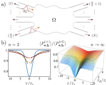
FIG. 1. a) Two bosonic wavepackets with mean velocityv, transversal channelsa= (a1, a2) and widths=vτsapproach the chaotic cavity Ω with mean position difference z =vτ. b) ratio hP(+)i/hP(cl)i, between the quantum and classical probabilities (averaged over mesoscopic fluctuations) to find the bosonic particles indifferentoutput channelsb. b) Left:
For singly-occupied wavepackets, n= 2 (with N = 4 chan- nels) we observe a generalized Hong-Ou-Mandel (HOM) pro- file that changes from Gaussian (dotted) to a universal ex- ponential (thin solid tails) as function of the cavity’s dwell time τd, with τd/τs = 0.1,2.5,5 (solid blue, dashed-dotted yellow, dashed red), Eqs. (10-12) withz =z12. Right: For n→ ∞, N =αnη,hP(+)ireaches its classical limit ifη >2 or trivially saturates due to the Bosonic Birthday Paradox for η <2. Forη= 2 the Quantum-Classical Transition shows an exponentiatedHOM-like profile, Eq. (16) withx= 0, α= 1.
cupations [15], chaotic scattering [16] and detection [17], mesoscopic scattering of BECs contains all prerequisites of a realistic platform for BS, its certification [19], and related tasks [20]. This is illustrated with the recent real- ization of the two-particle HOM effect using atomic beam splitters in [18].
Since the methods developed for the study of MB scat-
arXiv:1409.1558v2 [quant-ph] 14 Apr 2016
tering of photons [23–27] ignore mesoscopic effects and physical scales like the cavity’s dwell time, we fill this gap and present analytic results on coherent MB scat- tering in the mesoscopic regime, particularly the way the QCT is affected by large occupation numbers and mesoscopic fluctuations. Supported by the universal cor- relations of SP scattering matrices [28, 29] responsible for characteristic mesoscopic wave interference effects like weak localization [30] and universal conductance fluctua- tions [31], we address the emergence of universal MB cor- relations due to the interplay between classical ergodicity, SP interference and quantum indistinguishability well be- yond the standard semiclassical SP picture [32]. Despite their intrinsically non-classical character, here MB corre- lations are successfully expressed and computed within a semiclassical approach in terms of interfering SP classical paths in the spirit of the Feynman path integral [33] by a one-to-one correspondence between MB classical paths (illustrated in Fig. 2) and terms of the expansion of the MB scattering probabilities. Our complete enumeration and classification of the MB paths allows for an explicit analysis of emergent phenomena in the thermodynamic many-particle limit, something out of reach of leading- order Random Matrix Theory (RMT) methods [34–36].
We also show here how mesoscopic dephasing effects encoded in the dwell time lead eventually to a univer- sal HOM profile, and provide a mesoscopic approach to the Bosonic Birthday Paradox (BBP) that constrains the experimental realization of BS due to a counter-intuitive scaling of coincidence probabilities with the density of particles [37]. Our methods can be extended to the opti- cal case by using the dispersion relation for photons and changing the cavity Ω to a multi-port waveguide network, making a connection with recent experiments [6–9].
The set up of the mesoscopic many-body scattering problem is depicted in Fig. 1(a). The incoming parti- cles (i= 1, . . . , n) with positions (xi, yi) occupy SP states represented by normalized wavepackets
φi(xi, yi)∝e−ikxiX(xi−zi)χai(yi). (1) The longitudinal wavepackets e−ikxX(x−z) have vari- ance s2, mean initial positionz s, and approach the cavity Ω with mean momentum ~k = mv > 0 along the longitudinal directions −xi. The relative positions of the incoming particles are then parametrized by the differences zij = zi −zj or delay times τij = zij/v.
The transverse wavefunction in the incoming channel ai∈ {1, . . . , N/2}isχai(yi) and has energyEχ, assumed for simplicity to be identical for all channels.
If the particles are identical, quantum indistinguisha- bility demands their joint state to be symmetrized ac- cording to their spin [38]. Introducing =−1 (+1) for fermions (bosons), the symmetrized amplitude to find the particles leaving in channels b= (b1, . . . , bn) with ener- gies E= (E1, . . . , En) is given by a sum over the action
of then! elementsP of the permutation group, A()a,b(E) =X
P
PAa,Pb(PE) (2) on the scattering amplitude for distinguishable particles,
Aa,b(E) =
n
Y
i=1
rm
~
e−i(k−qi)zi
√2π~qi
X(k˜ −qi)σbi,ai(Ei) (3)
where~qi=p
2m(Ei−Eχ) and ˜X(k) =R
e−ikxX(x)dx.
When n = 1, Eq. (3) formally defines the SP scatter- ing matrix σb,a(E) connecting the incoming and outgo- ing channels a and b. With these definitions, the MB probability to find the particles leaving in channelsbbut regardless of their energies is given by
Pa,b() = 1 a!b!
Z ∞ Eχ
dE|A()a,b(E)|2 (4)
= 1
a!b!
X
P,P0
P+P0 Z ∞
Eχ
dEAa,Pb(PE)A∗a,P0b(P0E).
Equation (4) includes the normalization factors o! = Q
imul(oi)!, where mul(oi) is the multiplicity of the chan- nel indexoi, in order to havePn
b1≤...≤bnPa,b() = 1.
Due to interference between different (P 6= P0) dis- tinguishable MB configurations,Pa,b() is sensitive to the relative positions of the incoming wavepacketszij. This dependence drives a transition from indistinguishability to effective distinguishability forzij → ∞. MB interfer- ence due to indistinguishability is thus intrinsically de- phased and one observes an effective QCT [8, 9], as seen from the HOM scenario [1] whereσisE-independent and 2n= 4 =N. In this case we get, using Eq. (4),
PaHOM16=a2,b16=b2 =|[σ]|2+ 1
2 +|[σ]|2−1
2 F2(z12), (5) where [·] denotes permanent (unsigned determinant) and
F(z) = Z ∞
−∞
X(x)X(x−z)dx , (6) satisfyingF(0) = 1,F(∞) = 0 is responsible for the non- universal profile of the QCT, as shown in the dotted curve in the left panel of Fig. 1(b) for Gaussian wavepackets.
Individual σ-matrices with specific entries leading to Eq. (5) and its few-particle generalizations are routinely constructed in arrays of beam splitters connecting waveg- uides for photonic systems [6, 7, 24, 25] and in quan- tum point contacts for electrons occupying edge states [39, 40]. Thanks to the Bohigas-Gianonni-Schmidt con- jecture, replacing the beam splitter or point contact by a chaotic mesoscopic cavity allows to sample the moments hf(σ)µiof any observablef(σ) over the full ensemble of random, unitary matricesσby sampling over energy win- dows or small variations of the cavity [14]. In this case
(a) ...
...
(b) ...
...
(c) ...
...
(d) ...
...
(e) ...
...
(f) ...
...
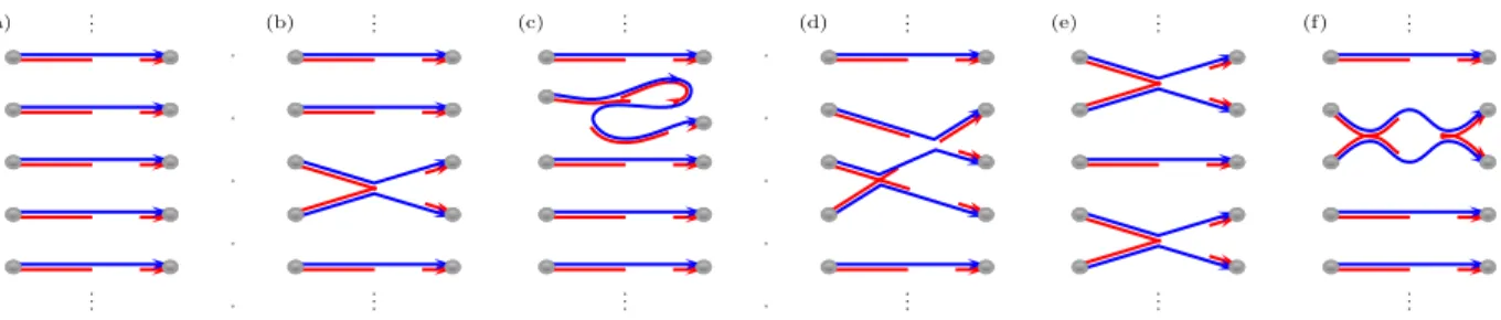
FIG. 2. Sets of interfering SP paths required for calculating MB transition probabilities, here forn= 5. In (a), both SP and MB correlations are neglected. In (c), weak localization at the SP level is included. For (b,d,e), and (f) only MB correlations are included. Combined SP and MB effects appear when the links in a MB diagram are decorated with SP loops.
averages of the form hσb,a(E)σ∗b0,a0(E0)i display univer- sal features depending only on the presence or absence of time reversal invariance, denoted as the orthogonal (β = 1) and unitary (β = 2) case. Interference effects in SP scattering probabilities are semiclassically under- stood in terms of statistical correlations among classical actions [28–31, 41] and here we generalize these methods.
We will mainly focus in the case, denoted byb, where every output channel is singly occupied; forβ = 1 we also demand that the in and outgoing channels are different.
In our approach any 2nµ-order correlator of σ-matrices appearing in the momentsh|Pa,b()(E)|2µiof the distribu- tion of scattering probabilities, Eq. (4), is given by an infinite diagrammatic expansion with terms that can be visualized as a set of links joining nµ in and outgoing channels, see Fig. 2. For the averaged transition proba- bility,µ= 1, the classical limit
hPa,b(cl)i= (n!/b!)N−n (7) for general b, is obtained from the trivial topology in Fig. 2(a) [43]. In Eq. (7)N is the number of open chan- nels at the mean initial SP energy U = mv2/2 +Eχ. Quantum effects at the SP level, in the spirit of [29, 30], give the sole contribution forP =P0 in Eq. (4) and are generated by adding SP loops to the links, as in Fig. 2(c).
These terms, independent of, can be evaluated up to in- finite order to give (withhPa,b(cl)i=n!N−n)
hPa,b(SP)i=hPa,b(cl)i(1−(1−2/β)/N)−n. (8) To calculatehPa,b()iwe must include genuine MB effects characterized by correlations between different SP paths, P 6= P0. The first MB diagrams without SP loops are depicted in Figs. 2 (b), (d), (e) while Fig. 2(f) shows the diagram (b) with a loop between 2 particles. The basic correlator in Fig. 2(b) involving a single pair of correlated paths is [31, 44]
hσbi,ai(Ei)σbj,aj(Ej)σb∗i,aj(Ej)σb∗j,ai(Ei)i (9)
= 1 N3
~2
~2+τd2(Ei−Ej)2 +O 1
N4
,
where τd is the dwell time, the average time a particle with energy (Ei+Ej)/2 remains within Ω. Taking into account only pairs of correlated paths, Eq. (4) gives [45]
hPa,b()i
hPa,bcl i= hPa,b(SP)i hPa,bcl i −
N
n
X
i<j
Q(2)(zij) +O 1
N2
, (10) with the generalized overlap integral Eq. (6),
Q(2)(z) = Z ∞
−∞
F2(z−vt)e−
|t|
τd
2τd
dt . (11) In order to study the impact of mesoscopic effects in the HOM scenario we taken= 2 and the sum in our Eq. (10) reduces to a single contribution withi= 1, j= 2. In the left pannel of Fig. 1(b) we plothPa,b()i/hPa,bcl ias function of the mismatch distancez=z12 between the incoming wavepackets in the case of broken time reversal invari- ance where Eq. (8) giveshPa,b(SP)i=hPa,b(cl)i. We see how mesoscopic effects produce universal deviations from the usual Gaussian profile, represented by the dotted line.
The functions Q(2) determine how the mismatch of arrival times dephases the MB correlations. We inter- pret Eqs. (10,11) as follows: Pairs of incoming particles that are effectively distinguishable get to interfere if their time delayτij in entering the cavity is compensated by the time τd the first particle is held within the meso- scopic scattering region. However, the interference gets weighted by the survival probability e−t/τd/τdof remain- ing inside the chaotic scatterer Ω. Universality of the dephasing of MB correlations is expected ifτd competes with the delay timesτij and widthsτs =s/v of the in- coming wavepackets, and leads to exponential tails in the interference profile for|zij| s. As shown in the left panel of Fig. 1(b) these exponential regions grow with the ratio τd/τs, while for τd ≤ τs QCT depends on the shape of the incoming wavepackets, as in Eq. (5),
Q(2)(z)
vτdvτs>k−1
−−−−−−−−−→ R∞
−∞F2(z)dzs
e−
|z|
vτd
2τd/τs vτsvτd>k−1
−−−−−−−−−→ F2(z).
(12) Mesoscopic dephasing of two-particle interference plays a fundamental role in the thermodynamic limitN, n →
∞ of the QCT through the mesoscopic version of the BBP [37] which constrains the scaling N = αnη in a way that hPa,b()i does not get trivially saturated either classically or by quantum bunching and antibunching [3, 10, 37, 46, 47]. To achieve a semiclassical theory of the mesoscopic BBP, in [48] we use RMT techniques to calcu- latehPa,b()i, which is only possible forzij = 0, τd/τs= 0.
We obtain the expression, valid for arbitrary, N, n,a,b ifβ= 2 and with the only conditiona∩b=∅ifβ= 1,
hPa,b()i
τd τs=0
zij=0= Wβ()(N, n)n!
Qn−1
l=0(N+l)(δ,++δ,−δb,b), (13) withδb,b= 1(0) ifbis (is not) singly-occupied and
W1()(N, n) = N+(n−1)
N+n+(n−1) ,W2()(N, n) = 1. (14) Equation (13) is a generalization for arbitraryβandof the bosonic, unitary case reported in [37]. A key obser- vation is that, contrary to the distinguishable (classical) case, Eq. (7), result (13) is constant over the MB final states forβ = 2. SP chaos leads then to full MB equili- bration for systems with broken time-reversal symmetry, providing dynamical support to the analysis of [37].
For singly-occupied statesb, Eqs. (7,13) give hPa,b()i
hPa,b(cl)i
!
τd τs=0
zij=0
−−−−−→n1 N=αnη
0 for η <2 e−2α1 for η= 2 1 for η >2,
(15) showing how in the thermodynamic limit scattering of identical particles is classical in the dilute limit η > 2, it gets saturated due to boson bunching and fermion an- tibunching even at zero densities ifη <2, and only the scaling N = αn2 gives a non-trivial limit. This is the essence of the BBP [10, 37, 46, 47], here derived from RMT (and for η > 1 from semiclassics) arguments for arbitrary β, . Forβ = 1, weak localization corrections to MB equilibration (akin to MB coherent backscattering [49]), to BS and to BBP are obtained from Eq. (13).
To address the interplay between intrinsic (zij 6= 0) and mesoscopic (τd/τs 6= 0) dephasing one must go be- yond RMT and we resort to semiclassical diagrammatics.
In [50] we study the semiclassical generating function for hPa,b()iand show that, order by order in the 1/N expan- sion, diagrams with pairwise correlations between parti- cles like Fig. 2(b),(e) dominate then→ ∞limit leading to Eq. (15) forη >1. The whole set of semiclasssical dia- grams with pairwise correlations can now be constructed forτd/τs>0 andzij 6= 0, and resumed to infinite order where the scalingη= 2 emerges [51].
If zij ∈ {0, z}, a situation that can be realized for bosons by injecting two wavepackets with macroscopic occupationsn(1±x)/2, we get [52]
hPa,b()i hPa,b(cl)i
−−−−−→n1
N=αn2 e−4α[(1+x2)Q(2)(0)+(1−x2)Q(2)(z)]. (16)
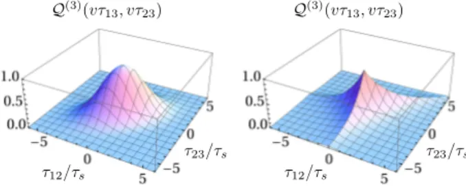
FIG. 3. Transition between the overlapping (τd/τs = 0.1, left) and the universal exponential (τd/τs= 2, right) regime for the three-body interference term, Eq. (17).
Remarkably then, for macroscopically populated incom- ing states we observe again a QCT driven by the ar- rival difference, with anexponentiatedHOM-like profile, as shown in Fig. 1(b, right) forx= 0 and α= 1.
Coming back to finite systems where MB interference is affected by other types of correlations, the diagram Fig. 2(d) containing three-body correlations gives
hPa,b()itriplets hPa,b(cl)i = 2
N2 X
i<j<k
Q(3)(zij, zkj), (17) with overlapping and exponential regimes given by
Q(3)(z, z0)
vτdvτs>k−1
−−−−−−−−−→ C(3) e
−3Max(z,z0,0) vτd
2τd/τs e
z+z0 vτd
2τd/τs,
vτsvτd>k−1
−−−−−−−−−→ F(z)F(z0)F(z−z0) (18) andC(3) =s−2R∞
−∞F(z)F(z0)F(z−z0)dzdz0. As shown in Fig. 3, this transition produces universal dephasing characterized by kinks with three-fold symmetry as a function of the time delay between incoming particles, consistent with the correlations measured in [9].
In conclusion, we have presented a semiclassical ap- proach to quantum scattering for Many-Body systems and used it to study the emergence of universal effects due to the interplay between Single-Particle classical chaos and quantum correlations coming from indistin- guishability. We have explicitly constructed the corre- lations responsible of Many-Body interference in meso- scopic scattering and computed their effect for both small and macroscopically large occupations in the thermo- dynamic limit, thus opening the possibility of trans- lating Boson Sampling, the Bosonic Birthday Paradox and related timely problems into experimentally acces- sible scenarios of chaotic scattering with massive parti- cles such as cold atoms, as outlined in the introduction.
Single-Particle chaos turns out to be sufficient to achieve Many-Body ergodicity, and this allows us to compute mesoscopic corrections to the Bosonic Birthday Para- dox. It leads to a sharp Quantum-Classical Transition in the thermodynamic limit and, under the scaling for the Quantum-Classical boundary, we found an exponen- tiated form of the Hong-Ou-Mandel profile.
Going beyond the first momenthPiof the distribution of scattering probabilities, in [53] we further calculate the leading order of the second momenthP2i. In fact, deter- mining just the leading order of higher moments should be pertinent for thePermanent Anti-Concentration Con- jecture important for Boson Sampling [10]. Intriguingly then, semiclassical diagrams and random matrices open up new avenues for understanding permanent statistics, while mesoscopic scattering of massive bosons appears as a promising candidate for their measurement.
We thank Andreas Buchleitner and Malte Tichy for in- structive discussions, and an anonymous referee for valu- able suggestions and for drawing our attention to refer- ences [21, 22].
[1] C. K. Hong, Z. Y. Ou, and L. Mandel,Phys. Rev. Lett.
59, 2044 (1987).
[2] Y.-S. Ra, M. C. Tichy, H. -T. Lim, O. Kwon, F. Mintert, A. Buchleitner, and Y. -H. Kim Proc. Natl. Acad. Sci.
USA110, 1227 (2013).
[3] M. Tillmann, B. Dakic, R. Heilmann, S. Nolte, A. Sza- meit, and P. Walther,Nature Photon.7, 540 (2013).
[4] M. A. Broome, A. Fedrizzi, S. Rahimi-Keshari, J. Dove, S. Aaronson, T. C. Ralph, and A. G. White,Science339, 794 (2013).
[5] A. Crespi, R. Osellame, R. Ramponi, D. J. Brod, E. F. Galvao, N. Spagnolo, C. Vitelli, E. Maiorino, P. Mataloni, and F. Sciarrino, Nature Photon. 7, 545 (2013).
[6] J. B. Spring, B. J. Metcalf, P. C. Humphreys, W. S. Kolthammer, X.-M. Jin, M. Barbieri, A. Datta, N. Thomas-Peter, N. K. Langford, D. Kundys, J. C. Gates, B. J. Smith, P. G. R. Smith, and I. A. Walm- sley, Science339, 798 (2013).
[7] B. J. Metcalf, N. Thomas-Peter, J. B. Spring, D. Kundys, M. A. Broome, P. Humphreys, X.-M. Jin, M. Barbieri, W. S. Kolthammer, J. C. Gates, B. J. Smith, N. K. Lang- ford, P. G. R. Smith, and I. A. Walmsley,Nature Comm.
4, 1356 (2013).
[8] Y.-S. Ra, M. C. Tichy, H.-T. Lim, O. Kwon, F. Mintert, A. Buchleitner, and Y.-H. Kim, Nature Commun. 4, (2013).
[9] M. Tillmann, S.-H. Tan, S. E. Stoeckl, B. C. Sanders, H. de Guise, R. Heilmann, S. Nolte, A. Szameit, and P. Walther,Phys. Rev. X5, 041015 (2015).
[10] S. Aaronson and A. Arkhipov, STOC ’11 43rd ann. ACM Symp. Theo. Comp.333, (2011).
[11] C. Shen, Z. Zhang, and L. Duan, Phys. Rev. Lett.112, 050504 (2014).
[12] T. Engl, J. D. Urbina, Q. Hummel, and K. Richter,Ann.
Phys.527, 737 (2014).
[13] B. Peropadre, A. Aspuru-Guzik, J. J. Garcia-Ripoll,Spin models and Boson SamplingarXiv:1509.02703 (2015).
[14] F. Haake, Quantum Signatures of Chaos, (Springer, Berlin) 2010.
[15] M. R. Andrews, C. G. Townsend, H. -J. Miesner, D. S. Durfee, D. M. Kurn, and W. Ketterle,Science275, 637 (1997).
[16] G. L. Gattobigio, A. Couvert, B. Georgeot, and D. Guery-OdelinPhys. Rev. Lett.107, 254104 (2011).
[17] J. F. Sherson, C. Weitenberg, M. Endres, M. Cheneau, I. Bloch, and S. KuhrNature467, 68 (2010).
[18] R. Lopes, A. Imanaliev, A. Aspect, M. Cheneau, D. Bo- iron, and C. I. Westbrook,Nature520, 66 (2015).
[19] M. Walschaers, J. Kuipers, J. D. Urbina, K. Mayer, M. C. Tichy, K. Richter, and A. Buchleitner, A sta- tistical Benchmark for Boson SamplingarXiv:1410.8547 (2014).
[20] Due to the formal analogy with photonic systems, in the limit of structureless cavities (τd → 0), our mesoscopic BS can be also used to implement tasks like simulating vibronic spectra in molecules [21] and generating massive path entanglement for metrology applications as in [22].
[21] J. Huh, G. G. Guerreschi, B. Peropadre, J. R. McClean, and A. Aspuru-Guzik,Nature Photon.9, 615 (2015).
[22] K. R. Motes, J. P. Olson, E. J. Rabeaux, J. P. Dowl- ing, S. J. Olson, and P. P. Rohde,Phys. Rev. Lett.114, 1708002 (2015).
[23] M. C. Tichy, M. Tiersch, F. de Melo, F. Mintert, and A. Buchleitner,Phys. Rev. Lett.104, 220405 (2010).
[24] S. Aaronson and A. Arkhipov,Quantum Info. Comput.
14, 1383 (2014).
[25] P. P. Rhode, K. R. Motes, and J. P. Dowling,Phys. Rev.
A91, 012342 (2015).
[26] C. Gogolin, M. Kliesch, L. Aolita, and J. Eis- ert, Boson-sampling in the light of sample complexity arXiv:1306.3995 (2013).
[27] V. S. Shchesnovich,Phys. Rev. A89, 022333 (2014).
[28] C. W. J. Beenakker,Rev. Mod. Phys.69, 731 (1997).
[29] G. Berkolaiko and J. Kuipers,Phys. Rev. E85, 045201 (2012);J. Math. Phys.54, 112103 (2013).
[30] K. Richter and M. Sieber, Phys. Rev. Lett. 89, 206801 (2002).
[31] S. M¨uller, S. Heusler, A. Altland, P. Braun, and F. Haake,New J. Phys.11, 103025 (2009).
[32] See for example R. K. Badhuri and M. BrackSemiclas- sical Physics, (Addison-Wesley, Reading) 1997.
[33] L. S. Schulman, Techniques and Applications of Path Integration, (John Wiley & Sons,New York) 1981;
M. Gutzwiller,Chaos in Classical and Quantum Mechan- ics, (Springer, New York) 1990.
[34] C. W. J. Beenakker, J. W. F. Venderbos, and M. P. van Exter,Phys. Rev. Lett.102, 193601 (2009).
[35] M. Cand and S. E. Skipetrov,Phys. Rev. A 87, 013846 (2013).
[36] M. Cand, A. Goetschy, and S. E. Skipetrov,EPL 107, 54004 (2014).
[37] A. Arkhipov and G. Kuperberg,Geom. and Topol. Mon.
18, 1 (2012).
[38] J. J. Sakurai, Modern Quantum Mechanics, Addison- Wesley (Reading) 1967.
[39] E. Bocquillon, V. Freulon, F. D. Parmentier, J.- M. Berroir, B. Placais, C. Wahl, J. Rech, T. Jonckheere, T. Martin, C. Grenier, D. Ferraro, P. Degiovanni, and G. Feve,Annalen der Physik526, 1 (2014).
[40] C. W. J. Beenakker, C. Emary, M. Kindermann, and J. L. van Velsen,Phys. Rev. Lett.91, 147901 (2003).
[41] D. Waltner, Semiclassical approach to mesoscopic sys- tems, (Springer, Heidelberg) 2012.
[42] Supplementary material [43] See [42] Sec. III, Eq. (68).
[44] J. Kuipers and M. Sieber, Phys. Rev. E 77, 046219
(2008).
[45] See [42] Sec. I, Eqs. (19–21).
[46] M. C. Tichy, K. Mayer, A. Buchleitner, and K. Molmer, Phys. Rev. Lett.113, 020502 (2014).
[47] V. S. Shchesnovich,Conditions for experimental Boson- Sampling computer to disprove the Extended Church- Turing thesis, arXiv:1403.4459 (2014).
[48] See [42] Sec. II, Eqs. (33, 36, 42, 45).
[49] T. Engl, J. Dujardin, A. Arguelles, P. Schlagheck, K. Richter, and J. D. Urbina, Phys. Rev. Lett. 112, 140403 (2014).
[50] See [42] Sec. IV A [51] See [42] Sec. IV B [52] See [42] Sec. IV C [53] See [42] Sec. III D
Supplementary material to the paper
”Multiparticle correlations in complex scattering:
birthday paradox and Hong-Ou-Mandel profiles in mesoscopic systems”
INTRODUCTION
The statistical study of quantum correlations due to indistinguishability in MB mesoscopic scattering can be carried out in two different, complementary ways. The powerful random matrix theory techniques introduced in Sec. II are suitable to address the universal regime where Hong-Ou-Mandel (HOM) effects can be neglected, namely, when the incoming wavepackets are mathemat- ically taken as plane waves without a well defined po- sition. Within random matrix theory, therefore, the ef- fect of finite dwell time in the HOM profile is by def- inition irrelevant. In order to study the emergence of universality due to chaotic scattering on HOM profiles and the quantum-classical transition due to effective dis- tinguishability, in Sec. III a semiclassical theory is imple- mented. The semiclassical approach is able to account for the effect of localized, shifted incoming wavepackets in the universal limit where only pairwise correlations are relevant, as shown in Sec. IV. Before that, in Sec, I the profile of the mesoscopic HOM effect is explicitly calcu- lated.
I. CALCULATION OF THE GENERALIZED OVERLAP INTEGRALS Q2(z)
Using the definition Eq. (4), the amplitudes given in Eq.(3) and the correlator in Eq. (9) of the main text, we get
Q(2)(z) = Z ∞
Eχ
dE1dE2
ei(q2−q1)z 1 +hτ
d(E1−E2)
~
i2 (19)
× m2 4π2~2
|X˜(k−q1)|2|X˜(k−q2)|2
~2q1q2 . To further proceed, we use Ei = Eχ +~2q2i/2m and q =q2−q1, Q = (q1+q2)/2. Then we observe that in the momentum representation the incoming wavepackets X˜(qi−k) are strongly localized aroundq1=q2=k. As long as ks1 we can extend the lower limit of the in- tegrals to −∞ and keep only terms of first order in q.
Under these conditions Eq. (19) yields Q(2)(z) =
Z ∞
−∞
dQdq eiqz
1 +v2τd2q2 (20)
×|X˜(Q−k−q/2)|2|X˜(Q−k+q/2)|2
4π2 ,
which can be finally transformed into Q(2)(z) =
Z ∞
−∞
F2(z−vt)e−|t|τd 2τd
dt . (21)
II. RMT APPROACH FOR TRANSMISSION PROBABILITIES
In this section we derive and then prove results for the transmission probabilities of bosons and fermions in both symmetry classes, Eq. (13) in the main text.
A. Bosons
Fornbosons, we start with the expression A˜+n = 1
√n!
X
P∈Sn n
Y
k=1
Zik,oP(k), (22) where we sum over all permutationsP of{1, . . . , n}and whereZ=σTis the transpose of the single particle scat- tering matrix σ (so we can identify the first subscript as an incoming channel and the second as an outgoing one). For simplicity we assume that all the channels are distinct. This quantity is related to then-particle ampli- tude when the particle energies coincide orτd= 0.
For the transmission probability we are interested in
|A˜+n|2= ˜A+n( ˜A+n)∗= 1 n!
X
P,P0∈Sn
n
Y
k=1
Zik,oP(k)Zi∗k,oP0(k). (23) The averages over scattering matrix elements are known both semiclassically and from RMT (see [54, 55] for ex- ample)
Za1,b1· · ·Zan,bnZα∗1,β1· · ·Zα∗n,βn
(24)
= X
σ,π∈Sn
VN(σ−1π)
n
Y
k=1
δ(ak−ασ(k))δ(bk¯−βπ(k)¯ ), where V are class coefficients which can be calculated recursively.
However, since the channels are distinct, for each pair of permutations P,P0 in Eq. (23) only the term with σ= id and π =P(P0)−1 in Eq. (24) contributes. One then obtains the result
P˜n+=h|A˜+n|2i= 1 n!
X
P,P0∈Sn
VN(τ), (25)
where
P˜n+= 1
n! hPa,b+ i
τd τs=0
zij=0 (26)
is the transmission probability when the particles enter at equal energies at the same time. In Eq. (25)τ =P(P0)−1 is the target permutation of the scattering matrix corre- lator. Sinceτis a product of two permutations, summing over the pairP,P0just means thatτ covers the space of permutationsn! times and
P˜n+ = X
τ∈Sn
VN(τ). (27)
Since the class coefficients only depend on the cycle type of τ, one could rewrite the sum in terms of partitions.
For this we let v be a vector whose elements vl count the number of cycles of length l in τ so that P
llvl = n. Accounting for the number of ways to arrange the n elements in cycles, one can write the correlator as
P˜n+=
P
llvl=n
X
v
n!VN(v) Q
llvlvl!, (28) where we represent the argument of V by the cycles en- coded inv.
Typically, one considers correlators with a fixed target permutation, rather than sums over correlators as here in Eq. (27). For example fixingτ = (1, . . . , n) provides the linear transport moments whileτ=idgives the mo- ments of the conductance. A summary of some of the transport quantities which have been treated with RMT and semiclassics can be found in [56].
1. Examples
Representing the argument of the class coefficientsVN
instead by its cycle type, one can directly write down the result forn= 1,2:
P˜1+=VN(1)
P˜2+=VN(1,1) +VN(2), (29) while forn= 3 there are 6 permutations
(1)(2)(3) (123) (132)
(1)(23) (12)(3) (13)(2), (30) and so
P˜3+=VN(1,1,1) + 3VN(2,1) + 2VN(3). (31) With the recursive results in [54, 55] for the class co- efficients we can easily find the following results for low n:
2. Unitary case
Without time reversal symmetry, the results are P˜1+= 1
N P˜2+= 1
N(N+ 1) P˜3+= 1
N(N+ 1)(N+ 2) P˜4+= 1
N(N+ 1)(N+ 2)(N+ 3)
P˜5+= 1
N(N+ 1)(N+ 2)(N+ 3)(N+ 4). (32) The pattern
P˜n+= Γ(N)
Γ(N+n). (33)
holds for all n as we prove in a following subsection.
In fact we can relate n! ˜Pn+ to the moments of a single element of a CUE random matrix and find a proof of Eq. (33) in [57].
For a comparison to diagrammatic results, the expan- sion inN−1is
P˜n+= 1
Nn −n(n−1)
2Nn+1 +. . . (34) 3. Orthogonal case
With time reversal symmetry, the results are P˜1+= 1
(N+ 1) P˜2+= 1
N(N+ 3) P˜3+= 1
N(N+ 1)(N+ 5) P˜4+= 1
N(N+ 1)(N+ 2)(N+ 7)
P˜5+= 1
N(N+ 1)(N+ 2)(N+ 3)(N+ 9), (35) with a general result of
P˜n+= Γ(N) Γ(N+n)
(N+n−1)
(N+ 2n−1), (36) and an expansion of
P˜n+= 1
Nn −n(n+ 1)
2Nn+1 +. . . . (37) For a proof of Eq. (36) we can show thatn! ˜Pn+ coincides exactly with the moments of a single element of a COE random matrix. The result as proved in [58] leads directly to Eq. (36).
B. Fermions Fornfermions we start instead with
A˜−n = 1
√n!
X
P∈Sn
(−1)P
n
Y
k=1
Zik,oP(k), (38) where (−1)P represents the sign of the permutation, counting a factor of -1 for each even length cycle in P.
Following the same steps for bosons, one has P˜n−=h|A˜−n|2i= X
τ∈Sn
(−1)τVN(τ), (39) so for example
P˜3−=VN(1,1,1)−3VN(2,1) + 2VN(3). (40) Calculating the class coefficients recursively one then finds the following results for lown:
1. Unitary case
Without time reversal symmetry, the results are P˜1−= 1
N P˜2−= 1
N(N−1) P˜3−= 1
N(N−1)(N−2) P˜4−= 1
N(N−1)(N−2)(N−3)
P˜5−= 1
N(N−1)(N−2)(N−3)(N−4), (41) The pattern turns out to be
P˜n−= Γ(N−n+ 1)
Γ(N+ 1) , (42)
and the expansion inN−1is P˜n−= 1
Nn +n(n−1)
2Nn+1 +. . . (43) 2. Orthogonal case
With time reversal symmetry, the results are P˜1−= 1
(N+ 1) P˜2−= 1
(N+ 1)N P˜3−= 1
(N+ 1)N(N−1) P˜4−= 1
(N+ 1)N(N−1)(N−2)
P˜5−= 1
(N+ 1)N(N−1)(N−2)(N−3) (44)
with a general result of
P˜n−=Γ(N−n+ 2)
Γ(N+ 2) (45)
and an expansion of P˜n+= 1
Nn +n(n−3)
2Nn+1 +. . . (46) C. Proofs
Now we can turn to proving the formulae in Eq. (42) and Eq. (45). These proofs build heavily on [58, 59] for the underlying details and methods. To introduce the techniques though, we start with the simpler case of re- proving Eq. (33).
1. Unitary bosons
Starting with the sum over permutations in Eq. (27), we use the fact that the class coefficients, which are also known as the unitary Weingarten functions admit the following expansion [59]
P˜n+= X
τ∈Sn
VN(τ) = 1 n!
X
λ`n
fλ Cλ(N)
X
σ∈Sn
χλ(σ), (47)
whereλis a partition ofnand the remaining term are as defined in [59]. To evaluate the sum we employ the char- acter theory for symmetric groups. The trivial character forSn isχ(n)(σ) = 1 forσ∈Sn while the orthogonality of irreducible characters means that
1 n!
X
σ∈Sn
χλ(σ)χµ(σ) =δλ,µ. (48)
Combining both these facts we have 1
n!
X
σ∈Sn
1χλ(σ) = X
σ∈Sn
χ(n)(σ)χλ(σ) =δ(n),λ. (49)
Substituting into Eq. (47) the gives P˜n+= 1
n!
X
λ`n
fλ
Cλ(N)δ(n),λ= f(n)
C(n)(N). (50) Sincef(n)= 1 andC(n)(N) =N(N+ 1). . .(N+n−1) from the definitions in [59] we obtain
P˜n+ = 1
N(N+ 1). . .(N+n−1), (51) recovering and proving Eq. (33).
2. Unitary fermions
For fermions we need to include the powers of (−1) in Eq. (39). For this we proceed as in the bosonic case, but now we for the powers of (−1) we use the irreducible characterχ(1n)(σ) = (−1)σ forσ∈Sn. Substituting into Eq. (39) gives
P˜n− = 1 n!
X
λ`n
fλ Cλ(N)
X
σ∈Sn
χ(1n)(σ)χλ(σ), (52) while orthogonality reduces the result to
P˜n−= 1 n!
X
λ`n
fλ
Cλ(N)δ(1n),λ= f(1n)
C(1n)(N). (53) Takingf(1n)= 1 andC(1n)(N) =N(N−1). . .(N−n+1) from the definitions in [59] we obtain
P˜n−= 1
N(N−1). . .(N−n+ 1), (54) proving Eq. (42).
3. Orthogonal fermions
This proof is somewhat more involved and we start by expressing our sum
P˜n−= X
τ∈Sn
(−1)τVN(τ)
=X
µ`n
n!
zµ
(−1)n−l(µ)WgO(µ;N+ 1), (55) in terms of WgO which are the Weingarten function for the COE and which are evaluated for permutationsτ of coset-typeµwhile zµ is as defined in [58]. As in [58] we can reexpress our sum in terms of double length permu- tations
P˜n− = 1 2nn!
X
σ∈S2n
−1 2
n−l0(σ)
WgO(σ;N+ 1), (56) wherel0(σ) is the length ofµ ifµis the coset-type ofσ.
From the definition of the orthogonal Weingarten func- tion [59] our sum becomes
P˜n−= 1 (2n)!
X
λ`n
f2λ Dλ(N+ 1)
X
σ∈S2n
−1 2
n−l0(σ)
ωλ(σ), (57) in terms of zonal spherical functionsωλ. These play the role of the irreducible characters used for the unitary case, and analogously as for the unitary fermions
ω(1n)(σ) =
−1 2
n−l0(σ)
. (58)
The zonal functions also follow an othogonality relation 1
(2n)!
X
σ∈S2n
ωλ(σ)ωµ(σ) = δλ,µ
f2λ , (59) so that
P˜n−=X
λ`n
f2λ Dλ(N+ 1)
δλ,(1n)
f2λ = 1
D(1n)(N+ 1). (60) Finally from the definition ofDλ(N+ 1) in [59] one has D(1n)(N+ 1) =Qn
i=1(N+ 1−i) giving P˜n− = 1
(N+ 1)N . . .(N−n+ 2), (61) proving Eq. (45).
D. Coinciding channels
We start with letting k outgoing channels (say bi, i = 1, . . . , k) be identical while keeping the remaining outgoing channels and the incoming channels distinct.
Then still only σ = id is permissible in Eq. (24) while πcan now take any value KP for allK ∈Sk. The sum becomes
Pˆn±= X
P∈Sn
(±1)P X
K∈Sk
VN(KP). (62) For eachK we setτ=KP then since
(±1)P = (±1)K−1τ= (±1)K−1(±1)τ = (±1)K(±1)τ, (63) the sum reduces to
Pˆn±= X
K∈Sk
(±1)K X
τ∈Sn
(±1)τVN(τ). (64) Since we already know the sum overτ
Pˆn±= X
K∈Sk
(±1)KP˜n±, (65) we are left with the simple sum over K. For bosons, this is simplyk! while for fermions we can again use the irreducible characters and their orthogonality
X
K∈Sk
(−1)K= X
K∈Sk
χ(1k)(K)χ(k)(K) =k!δ(1k),(k)=δk,1, (66) since clearly (1k) and (k) can only be the same partition whenk= 1. Combined we have
Pˆn± =k!(1±1) ˜Pn± k >1. (67) We can repeat this process for arbitrary sets of coincid- ing incoming and outgoing channels giving the result for bosons that ˆPn+ =a!b! ˜Pn+ and zero for fermions as soon
as any channels coincide. For the unitary case there is no restriction on whetheraorbcontain the same channels, but in the orthogonal case as soon as this happens the simple formula in Eq. (24) is no longer valid and must be replaced by a more complicated version (see [54, 55]
for example). With this restriction, these results provide Eq. (13) in the main text.
III. SEMICLASSICAL TREATMENT OF SCATTERING MATRIX CORRELATORS We will treat correlators of An using a semiclassical diagrammatic approach. This is heavily based on [55, 56, 60, 61] and we refer in particular to [55, 60] for the underlying details and methods.
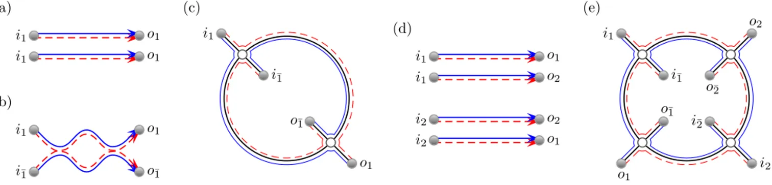
We return first to the transmission probability for bosons in Eq. (27). For a given cycle (1, . . . , l) in the target permutation τ the semiclassical trajectories have a very particular structure whereby we first travel along a trajectory with positive action fromi1 to o1 and then in reverse back along a trajectory with negative action to i2 and so on along a cycle until we return to i1. For example forn= 3 we have the trajectory connections in Fig. 4(a) for each target permutationτ in Eq. (30).
For the actions of the diagram to nearly cancel, and to obtain a semiclassical contribution, the trajectories must be nearly identical, except at small regions called encounters. By directly collapsing the trajectories onto each other, as in Fig. 4(b) we obtain some of the leading order diagrams for each τ. In fact for each diagram, following the rules of [62], the semiclassical contribution is a factor of−N for each encounter and a factor ofN−1 for each link between the encounters. For each cycle of lengthlin the diagrams in Fig. 4(b) one then has a factor of orderN−2l+1.
As a straightforward example we can look at the sim- plest diagrams made up of a set of independent links like the first diagram in Fig. 4(b). Withnlinks each provid- ing the factorN−1 we have the contribution
P˜±=N−n (68)
This contribution is in fact unaffected by the energy and time differences of the incoming particles leading directly to the classical contribution presented in Eq. (7) of the main text. This contribution also accounts for the leading order terms in the expansions of Eqs. (34), (37), (43) and (46).
A. Diagrammatic treatment without time reversal symmetry
Once the contribution of each diagram has been es- tablished, one then needs to generate all permissible di- agrams. As shown in [55, 61] however the vast majority
of semiclassical transport diagrams cancel. Those which remain can be untied until their target permutation be- comes identity. For systems without time reversal sym- metry, which we consider first, they can be mapped to primitive factorisations. One can reverse the process to build the diagrams by starting with a set of nindepen- dent links and tying together two outgoing channels into a new encounter. This tying process increases the or- der of the diagram by N−1. If the outgoing channels are labelled byj andkthen the target permutation also changes toτ(j k). For example going from the top left di- agram of Fig. 4(b) tying together any two outgoing chan- nels leads to the three example along the bottom row.
The diagrams correspondingly move from orderN−3 to N−4.
Tying the remaining outgoing channel to one of those already tied leads to a diagram of the type further along the top row of Fig. 4(b) [for each of which there are 3 possible arrangements, and an alternative with a single larger encounter] and now of orderN−5.
Of course one could retie the same pair chosen in the first step, so that the target permutation is again identity.
Such a diagram is however not shown in Fig. 4(b) but can be thought of as a higher order correction to a diagonal pair of trajectories. These types of diagrams appear when one treats the conductance variance for example. Such diagrams have a graphical interpretation which we will discuss below and use to generate them.
1. Forests
At leading order for each cycle of length l in τ the trajectories however form a ribbon graph in the shape of a tree. The tree has 2l leaves (vertices of degree 1) and all further vertices of even degree greater than 2. Such trees can be generated [63] by first treating unrooted trees whose contributions we store in the generating function f. Using the notation in [60], the function satisfies
f = r N −
∞
X
k=2
f2k−1, f N =
q
1 + 4rN22 −1
2r , (69)
where the power ofrcounts the number of leaves and the encounters may not touch the leads since the channels are distinct. Rooting the tree we add a leave to arrive at the generating functionF =rf while settingr2=swe arrive at
F N =
q
1 + N4s2 −1
2 . (70)
Expanding in powers ofs F = s
N − s2 N3 +2s3
N5 −5s4 N7 +14s5
N9 +. . . (71)
(a) i1
i2
i3
o1
o2
o3
i1
i2
i3
o1
o2
o3
i1
i2
i3
o1
o2
o3
i1
i2
i3
o1
o2
o3
i1
i2
i3
o1
o2
o3
i1
i2
i3
o1
o2
o3
(b) i1
i2
i3
o1
o2
o3
i1
i2
i3
o1
o2
o3
i1
i2
i3
o1
o2
o3
i1
i2
i3
o1
o2
o3
i1
i2
i3
o1
o2
o3
i1
i2
i3
o1
o2
o3
FIG. 4. (a) The permutations on 3 labels represented as trajectory diagrams. (b) Semiclassical contributions come when the trajectories are nearly identical, as when collapsed onto each other.
one has an alternating sequence of Catalan numbers, A000108 [64].
When summing over all permutations for τ, each cy- cle of length l can be arranged in (l−1)! ways and we now wish to include this factor in the ordinary generating function. First we divide instead by a factor l with the transformation
K0
N = Z F
sN ds= r
1 + 4s
N2 −1 (72)
+1 2ln
N4
1−q 1 + N4s2
2s2 +N2
s
, so thatK0becomes the exponential generating function of the leading order trees multiplied by the factor (l−1)!
as required. To now generate any forest of trees corre- sponding to all permutations τ we can exponentiateK0
to obtain the exponential generating function eK0−1 = s
N +(N−1)s2
2N3 +(N2−3N+ 4)s3 6N5 +(N3−6N2+ 19N−30)s4
24N7 +. . . (73) whose first few terms can be explicitly checked against diagrams.
2. Higher order corrections to trees
For each given cycle (1, . . . , l) of τ there are higher order (in N−1) corrections which can be organised in a diagrammatic expansion [56, 60]. For systems without time reversal symmetry, the first correction occurs two orders lower than leading order and the corresponding diagrams can be generated by grafting the unrooted trees on two particular base diagrams. Repeating the steps in [60], while excluding the possibility for encounters to touch the leads (since the channels are distinct), one first
obtains
K2=−(f2+ 3)f4
6(f2+ 1)3 , (74) where handily, the method for subleading corrections au- tomatically undercounts by a factor of l so we directly obtain the required exponential generating function. Fi- nally we substitute from Eq. (69) and find
12N K2= 1 + N6s2
1 +N4s2
32 −1. (75) The exponential generating function eK0+K2 −1 would then generate all corresponding diagram sets up to this order.
3. Other corrections
However, the higher order corrections to trees are less important than the higher order corrections to other target permutation structures. For any pair of cycles (1, . . . , k)(k+ 1, . . . , l) inτ we can have diagrams which are orderN−2smaller than a pair of leading order trees.
For example, tying any two outgoing channels of a tree on the cycle (1, . . . , l) would break the target permutation into two as here.
To generate diagrams with two cycles, we graft trees around both sides of a circle as for the cross correlation of transport moments treated in [60]. This will include the example withn = 3 mentioned at the start of this subsection.
Following the steps in [60], while excluding the possi- bility of encounters touching the lead, one finds the gen- erating function
κ=−ln
1−f12f22 (1−f12)2(1−f22)2
(76) + ln
1 (1−f12)2
+ ln
1 (1−f22)2
,