Optimization of the z-Vertex Neural Network Trigger for the Belle II Experiment

(1)

Optimization of the z-Vertex Neural Network Trigger for the

Belle II Experiment

Sara McCarney

Munich 2019

(2)

(3)

Optimization of the z-Vertex Neural Network Trigger for the

Belle II Experiment

Sara McCarney

Master Thesis

at the Faculty of Physics

of Ludwig–Maximilians–Universit¨ at Munich

submitted by Sara McCarney

from Belfast, Northern Ireland

Munich, 08.08.2019

(4)

(5)

Optimierung des Neuronalen z-Vertex Trigger f¨ ur

das Belle II Experiment

Sara McCarney

Masterarbeit

an der Fakult¨ at f¨ ur Physik

der Ludwig–Maximilians–Universit¨ at M¨ unchen

vorgelegt von Sara McCarney aus Belfast, Nordirland

M¨ unchen, den 08.08.2019

(6)

(7)

Declaration:

I hereby declare that this thesis is my own work, and that I have not used any sources and aids other than those stated in the thesis.

M¨ unchen, 08.08.2019

(8)

(9)

List of Figures

1. Belle background . . . xxii

1.1. The Standard Model . . . 2

1.2. Parity Transformation . . . 3

1.3. GIM Mechanism . . . 4

1.4. Unitarity Triangle . . . 6

1.5. B-meson decay at Belle II . . . 8

2.1. SuperKEKB collider . . . 12

2.2. Nanobeam scheme . . . 14

2.3. Belle II Detector . . . 15

2.4. Drift Cell of CDC . . . 16

2.5. CDC Wire conguration . . . 17

2.6. CDC Wire Orientations . . . 17

3.1. L1 track trigger pipeline . . . 22

3.2. Track segment shapes . . . 23

3.3. Track segment left/right determination . . . 24

3.4. 2D Hough transformation . . . 25

3.5. Neurotrigger input . . . 26

3.6. Crossing point of 2D track with CDC wire layer in transverse plane . . . 28

4.1. Multi Layer Perceptron Architecture . . . 30

4.2. Training and validation errors . . . 32

5.1. Distribution ofz-vertex values for the Standard network . . . 36

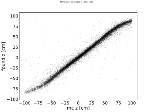
5.2. Scatter plot of found z and true z-vertex values for the Standard network 36 5.3. Resolutions of the Standard network . . . 37

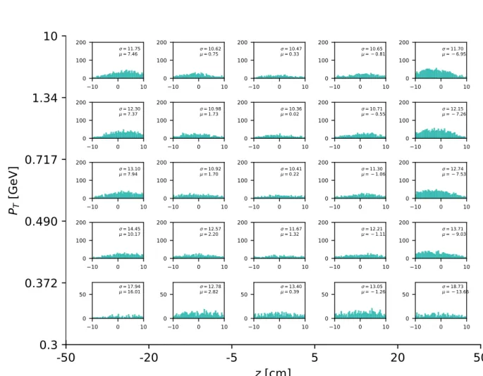
5.4. Resolutions dependent on the p_t and true z values of the Standard network 38 5.5. pt-dependent resolutions with Phase 2 background . . . 39

5.6. p_t-dependent resolutions with Phase 3 background . . . 40

5.7. p_t-resolutions of ETF Phase 2 . . . 42

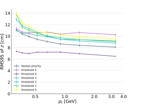
5.8. p_t-resolutions of ETF Phase 3 . . . 43

5.9. Left/right efficiency . . . 44

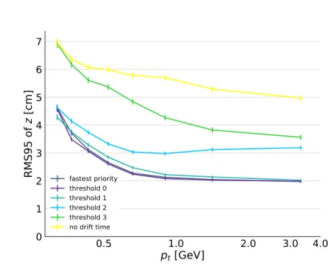
5.10.p_t-dependent resolutions for Ignore Left/right and No Drift times . . . . 44

5.11.p_t-dependent resolution with more hidden nodes . . . 45

5.12. Distribution ofz-vertex values along the ±100 cm range . . . 46 5.13. Scatter plot of found z and true z-vertex values along the±100 cm range 47

(14)

5.14. Distribution of z-vertices along the±100 cm range . . . 47

5.15.p_t-dependent resolution for Reco Tracks . . . 48

A.1. Dataset structure in the CDCTriggerNeuroTrainer module . . . 53

B.1. Training data for Standard network . . . 61

B.2. Resolutions dependent on the p_t and truez values of the Standard network 62 B.3. Standard network error curves & test with real data . . . 63

B.4. Distribution & Resolution plots for Standard network tested with Phase 2 Background . . . 64

B.5. Distribution & Resolution plots for Standard network tested with Phase 3 Background . . . 65

B.6. Resolutions dependent on the p_t and truez values of the No Background network with Phase 2 Background . . . 66

B.7. No background network error curves & test with real data . . . 67

B.8. Distribution & Resolution plots for the No background network tested with Phase 2 Background . . . 68

B.9. Distribution & Resolution plots for the No background network tested with Phase 3 Background . . . 69

B.10.Resolutions dependent on the p_t and true z values of the Phase 3 network 70 B.11.Phase 3 network error curves & test with real data . . . 71

B.12.Distribution & Resolution plots for the Phase 3 network . . . 72

B.13.Resolutions dependent on the p_t and true z values of the ETF Phase 2 Threshold 0 network . . . 73

B.14.ETF Phase 2 Threshold 0 network . . . 74

B.15.Distribution & Resolution plots for the ETF Phase 2 Threshold 0 network 75 B.16.Resolutions dependent on the p_t and true z values of the ETF Phase 2 Threshold 0 network . . . 76

B.17.ETF Phase 2 Threshold 1 network error curves & test with real data . . 77

(15)

List of Figures xv

B.29.ETF Phase 3 Threshold 1 network error curves & test with real data . . 89 B.30.Distribution & Resolution plots for the ETF Phase 3 Threshold 1 network 90 B.31.Resolutions dependent on the p_t and true z values of the ETF Phase 3

Threshold 2 network . . . 91 B.32.ETF Phase 3 Threshold 2 network error curves & test with real data . . 92 B.33.Distribution & Resolution plots for the ETF Phase 3 Threshold 2 network 93 B.34.Resolutions dependent on the p_t and true z values of the ETF Phase 3

Threshold 5 network . . . 100 B.41.ETF Phase 3 Threshold 5 network error curves & test with real data . . 101 B.42.Distribution & Resolution plots for the ETF Phase 3 Threshold 5 network 102 B.43.Resolutions dependent on the p_t and true z values of the No Drift time

network . . . 103 B.44.No Drift time network error curves & test with real data . . . 104 B.45.Distribution & Resolution plots for the No Drift time network . . . 105 B.46.Resolutions dependent on thep_tand truezvalues of the Ignore Left/right

network . . . 106 B.47.Ignore Left/right network error curves & test with real data . . . 107 B.48.Distribution & Resolution plots for the Ignore Left/right network . . . . 108 B.49.Resolutions dependent on thep_tand truez values of the 127 nodes network109 B.50.127 nodes network error curves & test with real data . . . 110 B.51.Distribution & Resolution plots for the 127 nodes network . . . 111 B.52.Resolutions dependent on the p_t and true z values of thez100 network . 112 B.53.127 nodes network error curves & test with real data . . . 113 B.54.Distribution & Resolution plots for thez100 network . . . 114 B.55.Resolutions dependent on the p_t and true z values of the Reco Tracks

network . . . 115 B.56.Reco Tracks network error curves & test with real data . . . 116 B.57.Distribution & Resolution plots for the Reco Track network . . . 117

(16)

(17)

List of Tables

1.1. Meson constituents . . . 7

2.1. KEKB and SuperKEKB machine parameters . . . 14

2.2. Beampipe design parameters . . . 15

3.1. Differences in L1 trigger and HLT systems . . . 21

5.1. Event Time Finder Efficiency . . . 41

B.1. Particle Generation parameters that remained constant for all trainings . 61 B.2. Training parameters for the Standard network . . . 62

B.3. Training parameters for No Background network . . . 66

B.4. Training parameters for the Phase 3 network . . . 70

B.5. Training parameters for the ETF Phase 2 Threshold 0 network . . . 73

B.6. Training parameters for ETF Phase 2 Threshold 1 network . . . 76

B.10.Training parameters for ETF Phase 3 Threshold 1 network . . . 88

B.15.Training parameters for No Drift time network . . . 103

B.16.Training parameters for Ignore Left/right network . . . 106

B.17.Training parameters for 127 nodes network . . . 109

B.18.Training parameters for z100 network . . . 112

B.19.Training parameters for Reco Tracks network . . . 115

(18)

(19)

Abstract

For the Belle II experiment at the SuperKEKB asymmetric electron-positron (e⁺/e⁻) collider (KEK, Japan) the concept of a first level (L1) track trigger, realized by neural networks, is presented. Using the input from a traditional Hough-based 2D track finder, the stereo wire layers of the Belle II Central Drift Chamber are used to reconstruct by neural methods the origin of the tracks along the beam (z) direction. A z-trigger for Belle II is required to suppress the dominating background of tracks from outside of the collision point. This so-called Neurotrigger is based on a Multi-Layer Perceptron (MLP) Architecture and is implemented in FPGA hardware to trigger on events in real-time, satisfying a fixed latency budget of 300 ns. The Neural Networks are trained offline in a supervised learning process using Monte Carlo (MC) particles as targets. The full L1 track trigger can be simulated in software to obtain resolutions, comparing the ‘true’ MC values to the predicted values of the network. By means of these software simulations, one can find optimal parameters for the preprocessing and training of the Neurotrigger.

This thesis presents the results of such software simulations. Resolutions of ∼2 cm in the high particle transverse momentum (p_t) region, and ∼5 cm in the low p_t region are determined, sufficient for efficient background rejection. The importance of the selected drift time input algorithm on the optimal spatial resolution of thez-trigger and trainings for a preliminary z-cut of 40 cm are discussed.

(20)

(21)

Introduction

The Belle II Experiment at the SuperKEKB asymmetric electron-positron (e⁺/e⁻) collider (KEK, Japan) - a second-generation B-factory - aims to precisely measure CP- violation in the B-meson sector. Colliding e⁻ and e⁺ at respective beam energies of 7 GeV and 4 GeV, which corresponds to the Υ(4S) resonance, large quantities of B- meson pairs can be produced, allowing for the parameter space of the unitarity triangle to be further confined. With unprecedented sensitivity measurements, Belle II also aims to search for new physics (NP) beyond the Standard Model at the intensity frontier.

Following the success of its predecessor experiment Belle, the Belle II detector has been upgraded to include a new Pixel Detector (PXD) based on DEPFET technology and a larger Central Drift Chamber (CDC). KEKB is upgraded to SuperKEKB to reach peak luminosities of up to 8×10³⁵cm⁻²s⁻¹ and aims to achieve a total integrated luminosity sample of 50 ab⁻¹. With increasing beam currents and the new nanobeam scheme, the planned luminosity upgrade is expected to be accompanied by a strong increase in beam- induced background compared to Belle. In order to identify, for example, low charged track multiplicity events such asτ pairs, this background should be suppressed as much a possible.

Belle II’s trigger system aims then to discard a significant amount of this background at the first level trigger. By using the input from a traditional Hough-based 2D track finder, the stereo wire layers of the Belle II Central Drift Chamber are used to reconstruct in three dimensions and by neural methods the origin of the tracks along the beam (z) direction. A z-trigger for Belle II is required to suppress the dominating background of tracks from outside of the collision point. Belle did not employ a z-trigger, and as such their track trigger did not sufficiently reject an overwhelming quantity of background that originated outside the Interaction Point (IP), for example Bhabha tracks that hit accelerator structures, or Toushek effects from beam-induced background. A distribution of this background can be seen in Figure 1.

Since traditional track finding methods cannot be executed within the latency of the pipelined L1 trigger, a trigger based on neural networks (Neurotrigger) has been developed [2, 3, 4, 5] for implementation on FPGA hardware to operate in real time as part of the modular L1 track trigger. The Neurotrigger outputs z-Vertex and polar angle θ predictions. These outputs are sent to a Global Decision Logic (GDL) which makes a final decision on which events to keep. The goal of the Neurotrigger then is to discard events originiating outside a pre-determined ‘z-cut’, and to correctly identify those originating from the IP, which correspond to ‘interesting’ physics events.

The neural networks are trained offline in a supervised learning process with Monte Carlo (MC) particles used as training targets. The network weights are uploaded onto the hardware to trigger on events in realtime, with input values calculated in preprocess-

(22)

Figure 1.: Background distribution along z-axis in Belle [1]

ing steps on the FPGA. The full L1 track trigger up to and including the Neurotrigger may also be simulated in the software to determine resolutions and efficiencies, by comparing to the ‘true’ MC values to those predicted by the network. This is also used to debug the hardware, finding any discrepancies in results of the pipelined L1 track trigger algorithm and hardware implementations. This thesis presents the results of such software simulations. Resolutions were found to be dependent on particle transverse momentum (p_t) as expected due to a multiple scattering of particles. The networks achieve

∼2 cm resolutions in the high p_t region, and ∼5 cm in the low p_t region, sufficient for efficient background rejection. The importance of the selected drift time input algorithm on the optimal spatial resolution of the z-trigger and trainings for a preliminary z-cut of 40 cm are discussed.

As of April 2019, Belle II entered Phase 3, with first runs showing agreement with the simulation expectations. Improvement on z-cuts are expected to be made upon further optimization of the Neurotrigger.

This thesis will present some of the physics motivations behind the Belle II experiment in Chapter 1, including CP violation and rareτ-decays, before giving an overview of the SuperKEKB collider and the Belle II detector in Chapter 2. An overview of Belle II’s trigger system will be given in Chapter 3 , with focus on the L1 track trigger. Since the z-trigger component of the L1 track trigger is deployed with artificial neural networks, Chapter 4 provides an overview of the neural architecture and algorithms used to train the networks. The results of the software simulations of the Neurotrigger are presented in Chapter 5, with recommendations on optimal training parameters. Details of the software simulation methods, parameters and error calculations can be found in the Appendix.

(23)

1. Physics Motivations

Belle II operates at the Υ(4S) resonance -just above the threshold for B-meson pair production - producing large quantities of B-mesons in order to precisely measure CP- violation in the B-meson system. This is enabled by the relatively ‘clean’ environments at SuperKEKB which also provides a boost to the centre-of-mass (COM) system, enabling better resolution of decay parameters. Belle II will perform precision measurements aimed to test the standard model parameters, which could be indicative of new physics (NP) beyond the standard model, as well as providing constraints, and discriminating between, NP models [6]. This chapter gives an overview of the physics motivations for the Belle II upgrade, including CP-violation in the B-meson system and rare τ-decays.

1.1. The Standard Model

The standard model of particle physics (SM) is currently the best tested theory of subatomic physics that describes the elementary particles and the fundamental forces that govern their interactions. The elementary particles can be distinguished by their spin quantum number: fermions are half-integer spin particles while the bosons carry integer spin. The gauge bosons are spin-1 particles that mediate a force - the W and Z bosons mediate the Weak Interaction, the photon γ mediates the Electromagenetic Interaction and the gluons mediate the Strong Interaction. The Higgs boson, a spin- 0 boson, is responsible for the mass generation of heavy elementary particles and was discovered in 2012 at the Large Hadron Collider (LHC) by both the ATLAS and CMS experiments [7, 8].

The SM contains twelve fermions split into three generations of quarks (fermions that participate in the Strong Interaction) and leptons (fermions that do not participate in the Strong Interaction). Each generation consists of two particles leading to a total of six quark flavours (up, down, charm, strange, top and bottom) and six lepton flavours (electron, muon, tau and their corresponding neutrinos). Flavour physics concerns itself with the mixing of these so-called flavours. A summary of the SM can be seen in Figure 1.1.

(24)

u d

c s

t

quarks

b

e ν

_e

µ ν

_µ

τ ν

_τ

leptons

γ

g

Z

W

gaugebosons

H

up

down

charm

strange

top

bottom

electron electron neutrino

muon muon neutrino

tau tau neutrino

photon

gluon

Z boson

W^±boson

Higgs boson

Figure 1.1.: The elementary particles in the standard model of particle physics [9]

Although the SM is currently our best phenomenological theory of subatomic physics, many phenomena remain unexplained: the question of why there are only three generations of fermions, the origin of the hierarchy of mass, the absence of a dark matter candidate and the origin of neutrino mass are among the many open-ended questions the SM fails to answer. The Belle II Experiment aims to investigate some of these phenomena. In particular, Belle II will investigate the nature of CP-violation, which could hint to the unexplained asymmetry of matter and antimatter - that there is more matter observed in the universe and almost no antimatter. CP-violation is a necessary condition for this asymmetry, but the measured levels of CP-violation in the quark sector are far too small to compensate for the imbalance.

Symmetries and conservation laws play an important role in particle physics. Ac- cording to the famous Noether Theorem [10], conservation laws in physics are derived from an underlying symmetry. In the following we will discuss three fundamental (and discrete) symmetries, giving rise to surprising experimental findings and theoretical con- sequences. Violations of these symmetries are an essential ingredient to understand the working of the Weak Interaction, responsible for the transformation of flavour states.

1.1.1. Parity Transformation

Parity transformations are inversions at the origin of a coordinate system. Figure 1.2 shows an example of such an inversion, which is equivalent to a mirror reflection at the plane followed by a 180^◦ rotation around the axis orthogonal to the plane. Parity violation has not been observed in Strong and Electromagnetic interactions. The Weak Interaction, on the other hand, violates parity maximally, as demonstrated in the famous Wu Experiment conducted by C.S. Wu. Lee and Yang who proposed the violation of parity in the Weak Interaction, were awarded the Nobel prize in 1957 [11].

(25)

1.1 The Standard Model 3

x y

z

~_L

~p

y x z

~_L

~p

y x z

~_L

~p

Figure 1.2.: The effect of parity transformation, which is equivalent to a mirror reflection followed by a 180^◦ rotation about the mirror axis [9]

1.1.2. Charge Conjugation

Charge parity (C-parity), or charge conjugation, is also conserved in the Strong and Electromagnetic interactions. The C-parity operator transforms particles into their antiparticles with a change of sign of a generalised charge. The Electromagnetic charge, baryon number and the lepton number are among the charges which undergo a sign re- versal. C-parity is observationally maximally violated in the Weak Interaction - we see no left-handed anti-neutrinos and no right-handed neutrinos. What we do see, however, are left-handed neutrinos and right-handed anti-neutrinos, indicating the conservation of the combined Parity and Charge conjugation operators, (CP-conservation). Later we will see that this is also violated.

1.1.3. Cabibbo Angle & Discovery of new quarks

The left-handed states can transform into one another via the Weak Interaction and so are grouped into generation-wise doublets. In 1963, when only the up (u), down (d) and strange (s) quarks were known to exist, it was observed that the u-quark could transition, with different strength, to either a d-quark or an s-quark. Therefore, first proposed by N. Cabibbo [12], the eigenstates of the Weak Interaction were:

d⁰ =dcosθ_c+ssinθ_c (1.1)

where θ_c is the Cabibbo angle. On comparing the lifetimes of the charged pions and kaons, the Cabibbo angle was found to be θ_c ≈ 13.1^◦. However, the branching ratio of K_L⁰ −→ µ⁺µ⁻ was found to be much lower than expected. To explain this effect, the GIM Mechanism, proposed by Glashow, Iliopoulos and Maiani in 1970, introduced a fourth quark, named charm (c) [13]. There were now two left-handed interactions,

(26)

defining now a relation analogous to Equation 1.1, namely:

s⁰ =scosθ_c−dsinθ_c (1.2)

and the new weak doublet c

s

, the decay K_L⁰ −→ µ⁺µ⁻ could be suppressed with the addition of a second loop diagram as shown in Figure 1.3. The c-quark was experi- mentally verified several years later.

Figure 1.3.: The GIM Mechanism proposed a fourth quark, c, to achieve the required flavour-changing neutral current (FCNC) suppression (note the ‘-’ sign in the lower diagram in front of sin(θ_c), coupling the c-quark to the d-quark) Cabibbo’s mixing angle was thus extended to a matrix which described this coupling of u and c-quarks to mixed eigenstates of the d and s-quark (of the Weak interaction).

For two generations, the unitary 2×2 matrix was:

V_C =

cosθ_c sinθ_c

−sinθ_c cosθ_c

(1.3)

where the matrix VC operates on the d and s-quark states:

d’

s’

= V_C d

s

(1.4) In 1964, Christenson, Cronin, Fitch and Turlay proved CP-violation in the neutral kaon system, with their observation of two-pion decays in neutral kaon mixing of the K_L meson; to conserve CP, the K_L meson should only decay to three pions [14]. To explain this CP-violation within the SM, Kobayashi and Masakawa predicted a third generation of quarks, extending the Cabibbo matrix to the Cabibbo-Kobayashi-Masakawa (CKM) matrix, with a non-vanishing complex phase. The new quarks predicted by Kobayashi

(27)

1.1 The Standard Model 5

and Masakawa were discovered in 1975 (charm or c-quark), in 1977 (bottom or b-quark), and in 1995 the top (t-quark) was discovered at Fermilab [15, 16, 17, 18]. Kobayashi and Masakawa were awarded the Nobel prize for their bold conjecture in 2008, which was proven correct by the Belle and BaBar experiments [19, 20].

1.1.4. Cabibbo-Kobayashi-Masakawa Matrix

The CKM matrix elements can be labelled to represent the quark flavours involved in the charged current interactions:

V_CKM=





V_ud V_us V_ub V_cd V_cs V_cb V_td V_ts V_tb



 (1.5)

where V_CKM acts on the d, s and b mass eigenstates and d’, s’ and b’ are the flavour eigenstates which actually decay in the Weak Interaction:



 d’

s’

b’



= VCKM



 d s b



 (1.6)

As example, the element V_ub appear in the coupling of a b and u-quark to the W boson. V_CKM is a unitary, 3×3 matrix with three real parameters and an irreducible complex phase. Several unitarity relations therefore hold, one of which is the B-triangle, where the first column is multiplied with the complex conjugated last column. For CP- violation the complex phase must be non-vanishing. As can be seen in the Wolfenstein representation of the CMK matrix (see below), Vub and Vtd contain the complex phase.

However, the observed CP-violation within the quark sector that originates from the complex phase of the CKM matrix is many orders of magnitude too small to explain the dominance of matter in the universe. There must therefore be undiscovered sources of CP-violation.

1.1.5. Wolfenstein Parametrization & Unitarity triangle

In general, a unitary n×n matrix has n² free parameters. An orthogonal n×n matrix can be constructed from ¹₂n(n-1) real parameters usually written as angles describing the rotation. The remaining ¹₂n(n-1) free parameters are the complex phases, however only

1

2(n-1)(n-2) are physically observable phases that could lead to CP-violation. For a 3×3 unitary matrix, this leads to exactly one non-vanishing complex phase. A ‘standard’

parametrization of the CKM matrix is given by:

VCKM=





c₁₂c₁₃ s₁₂c₁₃ s₁₃e^−iδ

−s₁₂c₂₃−c₁₂s₂₃s₁₃eîδ c₁₂c₂₃−s₁₂s₂₃s₁₃eîδ s₂₃c₁₃ s₁₂s₂₃−c₁₂c₂₃s₁₃eîδ −c₁₂c₂₃−s₁₂c₂₃s₁₃eîδ c₂₃c₁₃



 (1.7)

(28)

where s_ij:= sinθ_ij, c_ij:= cosθ_ij and θ₁₂, θ₂₃ and θ₁₃ are the rotation angles where θ₁₂ is the Cabibbo angle and is the largest mixing angle in the CKM matrix. δ :=δ₁₃ is the complex phase leading to CP-violation.

Another common parametrization is the Wolfenstein Parametrization, which expands the CKM matrix in termns of the parameter λ = sinθ₁₂ ≈0.22 [21]. Wolfenstein then defined four parameters (λ, A,ρ, η):

λ= sinθ₁₂ Aλ² = sinθ₂₃ Aλ³(ρ−iη) = sinθ₁₂e^−iδ so that up to O(λ³), the CKM matrix can be written as:

V_CKM =





1− ¹₂λ² λ Aλ³(ρ−iη)

−λ 1− ¹₂λ² Aλ² Aλ³(1−ρ−iη) −Aλ² 1



 (1.8)

The advantage of this parametrization is that one can clearly see the hierarchy of the couplings - the largest couplings (O(1) belong to the same generation (along the diagonal) and the smallest couplings (O(λ³) are between the first and third generations of quarks. Note that the complex phase appears only in couplings of the order ofO(λ³), indicating that CP symmetry is violated weakly in the SM [9].

One can expand the unitarity conditions V_CKMV_CKM^†=1 up to O(λ³) which can be represented geometrically as a triangle on the complex plane. One particular orthogo- nality condition is interesting:

V_udV_ub^*+ V_cdV_cb^*+ V_tdV_tb^* = 0 = Aλ³(ρ−iη)−Aλ³+ Aλ³(1−ρ−iη) +O(λ⁵) (1.9) which contains three complex terms of O(λ³) that must form a closed triangle in the complex plane, as shown in Figure 1.4. It is convenient to normalize these terms so that one side is purely real with length 1. By measuring the internal angles of the triangle, one can test the unitarity of the CKM matrix, which is only unitary if the triangle closes.

This triangle is known at the B-triangle, since it includes the b-quark. An important property of this triangle is that the sides are all of the same order, which entails large CP-violating effects in the B-meson system.

ℜ ℑ

(ρ,η)

V_udV_ub^∗

−V_cdV_cb^∗ =ρ+iη

(1,0)

V_tdV_tb^∗

−V_cdV_cb^∗=1−ρ−iη

(0,0) ^VcdV_cb^∗

−V_cdV_cb^∗= −1 φ₃

φ₂

φ₁

Figure 1.4.: The unitarity condition can be represented as a triangle in the complex plane [9]

(29)

1.2 CP Violation 7

Mesons Antimesons

K sd K sd

B⁰_d bd B⁰_d bd

B⁰_s bs B⁰_s bs

D cu D cu

Table 1.1.: The mesons and their antiparticle constituents which exhibit mixing

1.2. CP Violation

A CP transformation combines the operators C and P successively, therefore interchang- ing a particle with its antiparticle and reversing the handedness of the particle. Therefore a CP transformation acts on a left-handed quark to produce a right-handed antiquark (q_L →q_R). Mesons then, which are bound states of a quark and an anti-quark, M = q₁q₂, are transformed to M = q₁q₂. Some meson constituents can be seen in Table 1.1.

CP is conserved in Strong and Electromagnetic interactions but violated in the Weak Interaction; CP-violation is a necessary condition to explain the observed asymmetry of matter and antimatter quantities in the universe [22]. The hadrons which exhibit mixing with their antiparticles are shown in Table 1.1. This section outlines CP-violation effects and ways to measure it.

1.2.1. Direct & Indirect CP Violation

Indirect CP-violation is related to the mixing of particles and antiparticles, and occurs when different probabilities or phases for the transitions hM|Mi 6= hM|Mi arises. For the neutral B-meson system, we have indirect CP-violation when hB₀|B₀i 6=hB₀|B₀i.

Direct CP-violation occurs in decays if|hf|Bi|² 6=|hf|Bi|² - that is when the transition probability of a meson decaying to a fermion it not equal to reverse process (an anti- meson decaying to an anti-fermion). This can happen for charged and neutral B-mesons.

A hybrid form of direct and indirect CP-violation can also occur whenever there is CP-violation in the interference between mixing and decay. All these observables will be measured at Belle II. The effect is small in the kaon sector but turned out to be much larger in the B-meson sector. Belle successfully measured this, however the statistics at Belle are not sufficient to see significant deviations from the SM, which must be there, albeit at very small levels.

1.2.2. CP Violation at Belle II

Running at the Υ(4S) resonance, the main decay mode at Belle II is B_d⁰B_d⁰. The boost in the COM frame, provided by the asymmetric COM energies of electron and positron collision, is transmitted to the B mesons. This is important in measuring asymmetries as a function of their decay length and allows for increased sensitivity to CP violating effects. A typical time-dependent CP-violation decay at Belle II of a B⁰B⁰ can be seen

(30)

in Figure 1.5 and time differences may be measured via the boosted decay points of the two B mesons to detect CP-violating effects.

Υ(4S) B_CP B_tag

e⁻ e⁺

boost

`⁻ J/ψ

µ⁻ µ⁺

K_S

π⁺ π⁻

∆z

∝(t_CP−ttag)

Figure 1.5.: Typical B⁰B⁰ decay for CP-violation measurements at Belle II [9]

For decays such as BCP→J/ΨKS, where BCPcan be a matter or antimatter particle, a flavour tagging procedure needs to be performed, where the algorithm looks for flavour- specific signatures, for example charged leptons in final state particles, in order to identify the flavour of Btag at the time of its decay. From this the flavour of BCP can also be determined, since the two B-mesons are in a coherent state of exactly one B⁰ and one B⁰ until one of them decays, at which point the remaining B-meson is free to oscillate between the flavours with a characteristic frequency. Thus flavour-tagging algorithms are very important for studying mixing and decay of neutral B-meson systems.

1.3. New Physics

Hadron colliders, such as the Large Hadron Collider (LHC) at CERN perform physics at the Energy Frontier, colliding particles at ever-increasing energies. SuperKEKB, on the other hand, will perform measurements at the Intensity Frontier, colliding particles at high luminosities and gathering high statistics. In addition to searching for CP- violation in the B-meson sector and other B-physics analyses, Belle II has an extenstive New Physics (NP) program that aims to over-confine SM parameters and search for hints of Physics Beyond the Standard Model (BSM). Such measurements include rare decays, strongly suppressed or forbidden in the SM, Electroweak processes and τ-physics. The following subsection gives an overview of the τ-physics program at Belle II which is tightly connected to the ability to construct an efficient track trigger for low charged multiplicity final states.

1.3.1. Lepton Flavour Violation

The discovery of neutrino oscillations was observed in 1998 at Super Kamiokande with the observation of ν_µ → ν_e. Neutrino oscillations occur when the flavour of a neutrino

(31)

1.3 New Physics 9

changes over large propagating distances. Neutrino oscillations necessitate a non-zero mass for the neutrinos and are therefore an extension to the Standard Model, where they are assumed to have zero mass. Neutrino oscillations can then be described in an analogous framework to CP-violation in the quark sector, with a Pontecorvo-Maki- Nakagawa-Sakata (PMNS) matrix to describe the mixing angles [23].

However, evidence for Lepton Flavour Violation (LFV) in the neutrino sector is highly suppressed because of the tiny masses of the neutrinos. Physicists then search for charged LFV, for example in the reaction τ → µγ. Belle II is ideal for such searches, since in the clean environments of e⁺/e⁻ colliders the initial state is well known.

Luckily,τ⁺τ⁻pairs have a cross-section of about 0.9 nb - the same order of magnitude as σ(BB). Enough τ-pairs should therefore be generated to hopefully observe LFV at Belle II. Since different BSM theories predict different branching fractions for the τ- decays, it would be possible to discriminate between some of these theories. In the case that no LFV is observed, experimental limits on the branching ratios can be determined.

The current branching fraction experimental limits [24] stand at

τ →µγ 4.4×10⁻⁸ (1.10)

τ →eγ 3.3×10⁻⁸ (1.11)

BB events typically produce ≈10 charged tracks, with approximately 3 to 9 of those visible in the L1 track trigger. Since rare τ-events have a low-multiplicity of tracks, the trigger threshold must be lowered below 3 tracks in order to observe these events.

Consequently, the L1 track trigger will see more background tracks, which should be suppressed at the first trigger level [3].

(32)

(33)

2. The Belle II Experiment

The Belle II Experiment is an international high-energy physics experiment located at the High Energy Accelerator Research Organization (KEK) in Tsukuba, Japan. The Belle II detector surrounds the collision point of the asymmetric SuperKEKB collider.

Traversing a 3 km circumference, SuperKEKB collides electron-positron (e⁺/e⁻) pairs at respective beam energies of 7 GeV and 4 GeV. Belle II, following its predeccessors Belle and BaBar, is a second-generation B-factory; large quantities of B mesons and their antiparticles are produced at the Υ(4S) resonance, enabling a precise measure- ment of CP-violation in the B meson system. This is enabled by the relatively ‘clean’

environments at SuperKEKB, as opposed to hadron colliders like LHCb [25]. Belle II will perform precision measurements aimed to find deviations from the Standard Model (SM), which would be indicative of new physics [6]. To achieve the target 50 ab⁻¹of total integrated luminosity, SuperKEKB and Belle II have been upgraded and designed ac- cordingly [26]. This section will outline SuperKEKB’s upgrade and design features, the various Belle II subdetectors and their principle of operation, and some of the expected sources of background, important to understand for an optimized design of experimental triggers.

2.1. SuperKEKB

SuperKEKB is an asymmetric e⁺/e⁻ collider, where asymmetric refers to the electron and positron energies of 7 GeV and 4 GeV, respectively, corresponding to a COM of the Υ(4S) mass. The enrgies can be tuned also reach higher and lower COMs. The double ring collider consists of an electron High Energy Ring (HER) and a positron Low Energy Ring (LER). The linear accelerator (LINAC) and 1 GeV positron Damping Ring (DR) provide the particles to be injected into the main rings. The LINAC accelerates bunches of e⁺/e⁻ to their target energies before they are injected into bunches in their respective storage rings. Positrons are passed through the DR before injection into the LER since they are produced with too large an emittance for the nanobeam scheme.

The electron and positron bunches collide at the Interaction Point (IP) at an angle of 83 mrad, allowing for ease of beam separation before and after collisions [9, 1]. A schematic of the SuperKEKB collider can be seen in Figure 2.1.

(34)

HER

e

⁻

LER e

⁺

e

⁻

e

⁺

e

⁺

/ e

⁻

IP

Figure 2.1.: Schematic of SuperKEKB collider located at KEK, Tsukuba - The Belle II detector surrounds the collision point of SuperKEKB

2.1.1. Beam Energies

SuperKEKB will operate primarily at the Υ(4S) resonance, which is the fourth radially- excited s-wave state of the Υ meson. Υ is the b¯b quarkonium, and at the Υ(4S) resonance, is just above the production threshold for B-meson pair production (m_B = 5.28 GeVc₀⁻², m_Υ(4S) = 10.58 GeVc₀⁻²). Υ(4S) therefore has a 96% chance of decaying to B meson pairs. B-meson pairs are produced almost at rest in the COM frame, meaning that the contributing momentum is almost entirely due to the boost of the asymmetric colliding energies. This nicely allows one to directly relate the distance ∆z between the decay vertices to the decay time difference ∆t:

∆t= ∆z

cβγ (2.1)

where c is the speed of light, γ is the Lorentz factor and β is the boost, which for a head-on collision is given by:

β= E_HER−E_LER EHER+ELER

R_φ_c (2.2)

where R_φ_c is a correction factor, accounting for the fact that the boost is actually slightly larger because of the finite crossing angle, φ_c of the e⁺/e⁻ beams. In order to achieve the design luminosity, the boost at SuperKEKB is reduced by a factor of ²₃ relative to KEKB. The average spatial distance ∆z between the B-meson decay vertices will consequently become smaller, but this is expected to be compensated, or even improved compared to KEKB, by the improved resolution of the vertex detector system (VXD, see below), as well as providing advantage for those decays with neutrinos in the final state which require good detector hermiticity [6].

(35)

2.1 SuperKEKB 13

2.1.2. Luminosity

SuperKEKB is designed to reach peak instantaneous luminosities of 8×10³⁵cm⁻²s⁻¹ - up to 40 times higher than its predecessor KEKB - and aims to collect over its lifetime over 50 ab⁻¹ of data. For two colliding beams the luminosity may be written as

L= N₊N−f

4πσ_xσ_y .R_L ∝ I₊I−

σ_xσ_y (2.3)

where the two transverse beam profiles are modelled as Gaussians with horizontal size σx and vertical size σy, N are the number of particles in the respective e⁺/e⁻ bunch, f is the crossing frequency of the bunches and R_L is a crossing factor which takes into account geometrical effects of the finite crossing angle and bunch length. One can see that the luminosity can therefore be increased by increasing the beam currents and by reducing the beam size.

Ideal particle trajectories perform closed orbits, returning to their initial start points after one revolution in the accelerator ring. In reality, however, these particles undergo oscillations around this closed orbit, so-called betatron oscillations. The horizontal and vertical beam sizes can then be written as

σ_x,y = q

_x,yβ_x,y(s) (2.4)

where is the emittance which measures how much the particles deviate from the ideal trajectory related to the beam divergence at initial injection and β_x,y(s) is the so-called β-function which varies according to the position s of the ideal orbit, and can be thought of as an envelope around all possible particle trajectories inside the beam.

This β-function depends strongly on the guide-field of the magnets around the ring and most importantly on the quadrupole magnets before and after the IP used to squeeze the beam.

The luminosity can be written in terms of the vertical beam-beam parameters ξ_y, which have the following scaling behaviour:

L ∝ I±ξy±

β_y ξy± ∝ N∓β_y

σ_yσ_x (2.5)

ξ_y describes the focusing force exerted on a bunch by the EM field of the opposite bunch. At low beam currents, ξy increases with the number of particles in a bunch. As currents increase, however, the beams influence each other to increase the emittance, which in turn increases the beam size. The ξ_y is said to saturate at this beam-beam limit. At this limit, the luminosity will depend only on the beam currents.

The novel nanobeam scheme, new to Belle II, avoids the problem of the hourglass effect that arises with the increase of our vertical β-function parameter by maximally reducing the overlap d of the beams down to 0.3 mm, 20 times smaller than KEKB.

This is achieved by the use of superconducting quadrupole magnets close to the IP. The

(36)

KEKB SuperKEKB

E_LER 3.5 GeV 4 GeV

E_HER 8 GeV 7 GeV

L 2.11×10³⁴cm⁻²s⁻¹ 8×10³⁵cm⁻²s⁻¹ σ_x 103/123µm 10.2/7.5µm

σ_y 2.9µm 59 nm

φ_c 22 mrad 83 mrad

boost βγ 0.425 0.287

Table 2.1.: Summary of main differences between KEKB and SuperKEKB machine parameters [1]

hourglass effect arises when the bunch lengthd > β_y, effectively reducing the luminosity.

The nanobeam scheme requires the beams to cross at a crossing angleφ_c, leading to an effective bunch length of

d= σ_x

sinφ_c (2.6)

and with the horizontal beam size σx ≈ 10µm, φc = 83 mrad, the hourglass require- ment is satisfied with d6β_y. Table 2.1 summarises the main differences between beam parameters of KEKB and SuperKEKB. A schematic of the nanobeam scheme can be seen in Figure 2.2. The first e⁺/e⁻ collisions were in March 2018, and March 2019 saw the first collisions with full detector geometry [27, 28].

x

z e

⁻

e

⁺

φ

_c

d

Figure 2.2.: The nanobeam scheme new to Belle II

2.2. Belle II Detector

The Belle II Detector is built to surround the interaction region of SuperKEKB and consists of several sub-detectors, all playing a role in particle tracking and identification.

The Belle II detector has a similar principle design to Belle, but has been upgraded in consideration of the higher currents, decreased beam sizes, modified interaction region

(37)

2.2 Belle II Detector 15

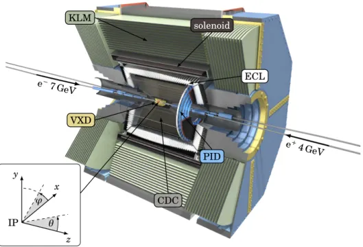
and the expected sizeable increase in background [1]. Figure 2.3 shows a schematic of the Belle II detector.

VXD

CDC

PID

ECL solenoid

KLM

e⁻7 GeV

e⁺4 GeV

θ ϕ

x IP

y

z

Figure 2.3.: THe Belle II detector and the coordinate system of Belle II

2.2.1. Beampipe

The beampipe follows the same principle design of Belle, consisting of two cylindrical Beryllium layers, separated by a gap for coolant and lined internally with gold plate to shield the detector from low energy X-rays. Beampipe radii are summarised in Table 2.2 [1].

Gold plate Thickness 10µm Inner Be pipe Inner radius 10.0 mm

Thickness 0.6 mm Gap for coolant Thickness 1.0 mm Outer Be pipe Outer radius 12.0 mm

Thickness 0.4 mm Table 2.2.: Beampipe design parameters

(38)

2.2.2. Vertex Detector

The Vertex Detector (VXD) has been upgraded from Belle to consist of a novel Pixel Detector (PXD) in addition to the Silicon Strip Detector (SVD). The PXD, based on DEPFET (DEPleted Field Effect Transistor) technology, is now the innermost sub- detector and directly surrounds the Interaction Point (IP). The VXD consists of 2 layers of PXD surrounded by 4 layers of SVD. Silicon strip layers alone were no longer sufficient for the IP due to the large occupancy caused by the luminosity upgrade [1]. Because of the reduced beam pipe radius, the first two detector layers are closer to the IP, and the outermost layer is also placed at a considerably larger radius. Subsequently, Belle II expects to see significant improvement in the vertex resolution, as well as in the reconstruction efficiency forK_S⁰ →π⁺π⁻ decays that have hits in the VXD [6].

2.2.3. Central Drift Chamber

The Central Drift Chamber (CDC) is the main tracking detector in the Belle II Exper- iment. The main purpose of the CDC is to precisely measure the momenta of charged particles by reconstructing charged tracks which curve in the presence of the 1.5 T field provided by the Belle superconducting solenoid.. In addition, it provides particle identification by measuring energy loss in its gas volume (the CDC can identify low momentum tracks that do not reach other sub-detectors). It is the sole input to the first level (L1) track trigger [1].

sense wire field wire drift circle

r ϕ

Figure 2.4.: Each sense wire is surrounded by 8 field wires to make up a ‘drift cell’

The CDC is a wire chamber consisting of 42240 field wires and 14366 sense wires con- taining a special gas mixture (50% C₂H₆ and 50% He). The wires are arranged radially in rectangular cells, with 8 field wires surrounding each sense wire and a high voltage applied between them. Charged particles passing through the chamber ionize the gas, as illustrated in Figure 2.4. Free electrons drift towards the sense wires, ionizing more gas atoms in the high electrical field surrounding the wire. This electron avalanche is registered as a hit whenever it reaches the sense wire, and a drift time can be determined (the time taken for the charged particle to reach the sense wire). In fact, the wire voltages and the gas mixture were specially selected so that the drift velocity remains

(39)

2.2 Belle II Detector 17

CDClayers

IP r

wires per layer:

SL 0 axial

160 SL 1 46 mrad

stereo

160 SL 2 axial

192 SL 3

−60 mrad stereo

224 SL 4 axial

256

SL 5 67 mrad

stereo

288 SL 6 axial

320

SL 7

−71 mrad stereo

352

SL 8 axial

384

Figure 2.5.: Layer configuration of the CDC with 9 superlayers - stereo angles within a superlayer vary by a few mrad; the given numbers are average values [9]

almost constant at 40µm ns⁻¹ for a wide range of locations inside the drift cells. Each sense wire in the chamber is assigned a unique ID number.

The 56 layers of wires in the chamber are arranged into 9 Superlayers (SL) totalling a cylindrical volume with an outer radius of 113 cm and an inner radius of 16 cm. The innermost SL consists of 8 layers of wires to cope with the higher background near the IP. The remaining SL have 6 layers of drift cells each. SL alternate between axial and stereo orientations as shown in Figure 2.5 and Figure 2.6. Axial wires are parallel to the z-axis, whilst stereo wires are inclined/skewed with respect to the beamline, allowing for a 3D reconstruction of tracks. The sign of the stereo wires alternate according to the so-called U,V orientations, giving the total configuration of all SL as AUAVAUAVA, with A the axial SL. Stereo SLs are skewed between 45.0 mrad to 74.0 mrad.

The measured CDC spatial resolution is ≈100µm. Viewed from the IP, the CDC covers a flat polar angle range of [17^◦, 150^◦]. The outer SL, again viewed from the IP, covers a polar angle of only [35^◦, 123^◦].

axial layer

x y

z

(a)

stereo layer

x y

z

(b)

Figure 2.6.: Wire orientations of CDC: (a) Axial wires are parallel to beamline (z-axis);

(b) Stereo wires are skewed with respect to beamline

(40)

2.2.4. Particle Identification System

In B factory detectors such as Belle II, particle identification (PID) is necessary for B- meson flavour tagging and to suppress background in precision measurements of B and D decays [29]. The newly developed PID system for Belle II consists of two indepen- dent Cherenkov detectors: a Time-of-Propogation (TOP) counter in the barrel region and an aerogel ring-imaging Cherenkov (ARICH) counter in the forward endcap region.

Their main task is to improve kaon and pion identification capabilities of the CDC by additionally imaging the Cherenkov rings produced [1] .

2.2.5. Electromagnetic Calorimeter

The goal of the Electromagnetic Calorimeter (ECL) is to detect photons and to identify electrons in order to discriminate them from hadrons, and in particular pions. High energy resolution and detection efficiency of photons is important in Belle II since one third of B-decay products are π⁰’s and other neutral products that produce photons [30]. It consists of a highly-segmented array of thallium doped caesium iodide CsI(TI) crystals in the barrel, forward and backward end-caps. CsI(TI) was chosen because of its ability to provide high light output via the thallium doping and because it has short radiation length of the CsI crystal [30].

2.2.6. K

L

-Muon Detector

Based on Resistive Plate Chambers (RPCs) and newly installed scintillator planes for the innermost layers, the new K_L-Muon (KLM) Detector is used in the barrel and endcap regions of Belle II and is the outermost detector. Designed to detect long-lived K⁰_L’s and muons and positioned outside of the solenoid coil, it consists of 4.7 cm thick iron plates alternating with active detector components, where the muons are visible as tracks.

Muon tracks in KLM can then be associated to a track in the CDC. The iron plates act as an absorber for hadronic particles and as the magnetic flux return yoke of the magnet. The ECL is surrounded by a superconducting coil, providing a field of 1.5 T parallel to the axial wires of the CDC (”the z-axis” in the Belle II coordinate system).

2.3. Beam-induced Background

Background rates at Belle II are expected to increase dramatically due to the luminosity upgrade. In order to discriminate background from real physics events, it is important to understand the different sources of background and their respective rates. Background sources at Belle II can in general be classified into two categories - collision-induced background (non-interesting physics plus secondary particles from non-relevant QED events such as Bhabha scattering) and beam-induced background (background originating from collisions of beam particles with gas molecules in the evacuated beam pipe or with components of the accelerator structures (beam pipe and magnet components)).

Beam-induced sources of background are discussed in this section.

(41)

2.3 Beam-induced Background 19

2.3.1. Beam-gas Scattering

Beam-gas scattering is caused by the scattering of beam particles by residual gas molecules in the beam pipe [6]. Bremsstrahlung and Coulomb radiations are the dominating sources of beam-induced gas background. Bremsstrahlung radiation refers to the emitted electromagnetic energy of a charged particle as it decelerates in the proximity of another charged high Z gas nucleus particle. Coulomb scattering refers to the scattering of charged particles as they come into contact with one of the gas nuclei at larger distances. Both these processes change the momenta of the beam particles - Bremsstrahlung decreases the energy of the beam particles whereas Coulomb scattering changes their direction. This enables vacuum chamber and magnet collisions which in turn produce particle showers. The size of these backgrounds depend on the beam current, the vacuum pressure in the rings and the material surrounding the magnets. Due to the very small radius of the beampipe at IP, the vacuum level around the IP is expected to be 100 to 1000 times worse than at KEKB [1]. The beam-gas Coulomb scattering rate is also expected to be a factor of 100 higher than at KEKB [6].

2.3.2. Touschek scattering

Another source of background is Touschek scattering [1]. Touschek scattering is intra- bunch scattering which changes the momenta of beam particles so that they can collide with the pipes and magnets, producing particle showers. This source of background is enhanced at SuperKEKB due to the new Nanobeam scheme [6]. This background is proportional to the beam bunch current, the number of bunches, and the inverse of the beam size and is studied by varying the HER or LER beam size [1]. Touschek background at Belle II is expected to be 20 times higher than at KEKB [6].

2.3.3. Bhabha scattering

Bhabha scattering refers to elastic scattering of electrons on positrons (e⁺e⁻ → e⁺e⁻), and was the dominant source of all backgrounds in Belle. Photons from these radiative Bhabha events propagate along the beam axis direction and interact with the iron in the magnets, which produces a large amount of neutrons via the giant photo-nuclear resonance mechanism (the main background source for the KLM). Belle II’s Bhabha rate is expected to be much lower than at KEKB because two separate quadrapole magnets are used. The Bhabha scattering rate is in fact used to measure luminosity since it is easy to identify and is a well understood QED process [1]. There are two Bhabha (further QED) channels that contribute in leading order:

2.3.4. Synchrotron Radiation

Synchrotron Radiation (SR) emitted from the beam is proportional to the beam energy squared and the magnetic field strength squared. Therefore the HER is the main source of SR. The inner surface of the beryllium beam pipe is coated with a gold layer to absorb

(42)

SR photons before they reach the VXD, since the SVD in Belle was severely damaged by SR photons with energies on the order of a few keV [6].

2.3.5. Two-photon Processes

A fifth contribution to beam background is the low momentum pair productione⁺e⁻ → e⁺e⁻e⁺e⁻ via the two-photon process. Due to the very large cross section for low secondary e⁺e⁻ pairs, this process can inject a large particle flux and consequently leave many hits in the inner Belle II detectors, and is the dominant source of background for the VXD [31].

2.3.6. Vacuum Scrubbing

Ultra-high vacuum is needed in particle accelerator rings in order to minimise the rate of beam-gas collisions. Vacuum scrubbing is a process by which the vacuum is improved over time, often months are needed.. Vacuum scrubbing works by simply allowing ‘wide’, unfocused beams with high currents to circulate in the rings in order to ‘knock out’ ad- sorbed molecules from the beampipe. Due to the upgraded LER, background is especially high there.

2.3.7. Background mixing

For this thesis, it is important to distinguish between two types of background: background hits and background tracks. Background tracks originate from processes described above and therefore do not come from the IP like the tracks from real physics events. If no information on the origin of these tracks is available at the trigger level, they will be considered as ‘real physics event’ and only recognized afterwards on the reconstruction level. The elimination of these background tracks already at the trigger level is the subject of this thesis. Single background hits, on the other hand, do not amount to tracks. Belle II expects to see a high number of these additional background hits, which may decrease the efficiency of the track finding in the trigger. Because of this problem the effects induced by the background hits need to be investigated carefully.

Simulation studies allow for a mixing of these background hits before CDC Digitiza- tion (the response of the CDC electronics) overlain with physics and real background events[9].

In this thesis, the terms ‘Phase 2’ and ‘Phase 3’ backgrounds are used to indicate the background campaigns simulated for expected levels of background at full luminosity of the respective Phase, which essentially amounts to more background hits mixed corresponding to the increased luminosity. Phase 3 is the first Physics run of the Belle II Experiment which began in March 2019 with full detector geometry [28]. Since Phase 3 has not yet reached full luminosity, Phase 2 is expected to suffice for the present studies.

See section 5.2 for related studies.

Optimization of the z-Vertex Neural Network Trigger for the Belle II Experiment

Optimization of the z-Vertex Neural Network Trigger for the

Belle II Experiment

Sara McCarney

Munich 2019

Optimization of the z-Vertex Neural Network Trigger for the

Belle II Experiment

Sara McCarney

Master Thesis

at the Faculty of Physics

of Ludwig–Maximilians–Universit¨ at Munich

submitted by Sara McCarney

from Belfast, Northern Ireland

Munich, 08.08.2019

Optimierung des Neuronalen z-Vertex Trigger f¨ ur

das Belle II Experiment

Sara McCarney

Masterarbeit

an der Fakult¨ at f¨ ur Physik

der Ludwig–Maximilians–Universit¨ at M¨ unchen

vorgelegt von Sara McCarney aus Belfast, Nordirland

M¨ unchen, den 08.08.2019

Declaration:

I hereby declare that this thesis is my own work, and that I have not used any sources and aids other than those stated in the thesis.

M¨ unchen, 08.08.2019

Contents

List of Figures

List of Tables

Abstract

Introduction

1. Physics Motivations

1.1. The Standard Model

u d

c s

t

b

e ν

µ ν

τ ν

γ

g

Z

W

H

1.1.1. Parity Transformation

1.1.2. Charge Conjugation

1.1.3. Cabibbo Angle & Discovery of new quarks

1.1.4. Cabibbo-Kobayashi-Masakawa Matrix

1.1.5. Wolfenstein Parametrization & Unitarity triangle

1.2. CP Violation

1.2.1. Direct & Indirect CP Violation

1.2.2. CP Violation at Belle II

1.3. New Physics

1.3.1. Lepton Flavour Violation

2. The Belle II Experiment

2.1. SuperKEKB

HER

e

LER e

e

e

e

/ e

IP

2.1.1. Beam Energies

2.1.2. Luminosity

x

z e

e

φ

d

2.2. Belle II Detector

2.2.1. Beampipe

2.2.2. Vertex Detector

2.2.3. Central Drift Chamber

2.2.4. Particle Identification System

2.2.5. Electromagnetic Calorimeter

2.2.6. K

-Muon Detector

2.3. Beam-induced Background