EUROPEAN ORGANISATION FOR NUCLEAR RESEARCH (CERN)
JHEP 06 (2021) 145
DOI:10.1007/JHEP06(2021)145
CERN-EP-2021-004 13th July 2021
Search for charged Higgs bosons decaying into a top quark and a bottom quark at √
𝒔=13 TeV with the ATLAS detector
The ATLAS Collaboration
A search for charged Higgs bosons decaying into a top quark and a bottom quark is presented.
The data analysed correspond to 139 fb
−1of proton–proton collisions at
√
𝑠
=13 TeV, recorded with the ATLAS detector at the LHC. The production of a heavy charged Higgs boson in association with a top quark and a bottom quark,
𝑝 𝑝 →𝑡 𝑏 𝐻+→𝑡 𝑏𝑡 𝑏, is explored in the
𝐻+mass range from 200 to 2000 GeV using final states with jets and one electron or muon. Events are categorised according to the multiplicity of jets and
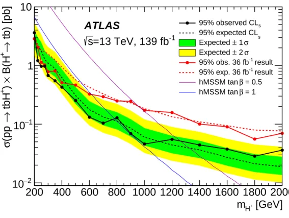
𝑏-tagged jets, and multivariate analysis techniques are used to discriminate between signal and background events. No significant excess above the background-only hypothesis is observed and exclusion limits are derived for the production cross-section times branching ratio of a charged Higgs boson as a function of its mass; they range from 3.6 pb at 200 GeV to 0.036 pb at 2000 GeV at 95% confidence level.
The results are interpreted in the hMSSM and
𝑀125ℎ
scenarios.
©2021 CERN for the benefit of the ATLAS Collaboration.
Reproduction of this article or parts of it is allowed as specified in the CC-BY-4.0 license.
arXiv:2102.10076v2 [hep-ex] 12 Jul 2021
Contents
1 Introduction 2
2 Data and simulation samples 3
3 Object reconstruction and event selection 5
4 Background modelling 7
5 Analysis strategy 8
6 Systematic uncertainties 11
7 Results 14
8 Conclusion 20
1 Introduction
The discovery of a Higgs boson with a measured mass of 125 GeV at the Large Hadron Collider (LHC) in 2012 [1–3] raises the question of whether this is the Higgs boson of the Standard Model (SM) or part of an extended scalar sector. Charged Higgs bosons
1are predicted in several extensions of the SM that add a second doublet [4–7] or triplets [8–12] to the scalar sector. In CP-conserving two-Higgs-doublet models (2HDMs), the properties of the charged Higgs boson depend on its mass, the mixing angle
𝛼of the neutral CP-even Higgs bosons, and the ratio of the vacuum expectation values of the two Higgs doublets (tan
𝛽).
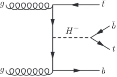
This analysis searches for charged Higgs bosons heavier than the top quark and decaying into a top quark and a bottom quark. At the LHC, charged Higgs bosons in this mass range are expected to be produced primarily in association with a top quark and a bottom quark [13], as illustrated in Figure 1.
Figure 1: Leading-order Feynman diagram for the production of a heavy charged Higgs boson in association with a top antiquark and a bottom quark, as well as its decay into a top quark and a bottom antiquark.
The ATLAS and CMS collaborations have searched for charged Higgs bosons in proton–proton (
𝑝 𝑝) collisions at
√
𝑠=
7
,8 and 13 TeV with data samples ranging from 2.9 to 36 fb
−1, probing the mass range below the top-quark mass in the
𝜏 𝜈[14–19],
𝑐 𝑠[20, 21], and
𝑐 𝑏[22] decay modes, as well as above the
1In the following, charged Higgs bosons are denoted𝐻+, with the charge-conjugate𝐻−always implied. Similarly, the difference between quarks and antiquarks𝑞and ¯𝑞is generally understood from the context, so that e.g.𝐻+→𝑡 𝑏means both𝐻+→𝑡𝑏¯ and𝐻−→¯𝑡 𝑏.
top-quark mass in the
𝜏 𝜈and
𝑡 𝑏decay modes [16, 18, 19, 23–27]. In addition,
𝐻+→𝑊 𝑍decays were searched for in the vector-boson-fusion production mode [28, 29]. ATLAS has also set limits on
𝐻+production in a search for dijet resonances in events with an isolated lepton using the Run 2 dataset [30].
No evidence of charged Higgs bosons was found in any of these searches.
This paper presents an updated search for
𝐻+production in the
𝐻+→𝑡 𝑏decay mode with the full Run 2 dataset of
𝑝 𝑝collisions taken at
√
𝑠=
13 TeV. This decay mode has the highest branching ratio for charged Higgs bosons above the top-quark mass [31]. Events with one charged lepton (
ℓ =𝑒, 𝜇) and jets in the final state are considered, and exclusive regions are defined according to the overall number of jets, and the number of jets tagged as containing a
𝑏-hadron. In order to separate signal from SM background, multivariate analysis (MVA) techniques combining jet multiplicities and several kinematic variables are employed in the regions where the signal rate is expected to be largest. Compared to the ATLAS result using 36 fb
−1of Run 2 data [25], improved limits on the
𝑝 𝑝→𝑡 𝑏 𝐻+production cross-section times the
𝐻+→𝑡 𝑏branching ratio are set by means of a simultaneous fit to the MVA classifier outputs in the different analysis regions, which determines both the contribution from the
𝐻+→𝑡 𝑏signal and the normalisation of the backgrounds. The improvement is small at low
𝐻+mass, where the measurement is dominated by systematic uncertainties, but larger than the simple scaling with the square root of the ratio of integrated luminosities at high
𝐻+mass. The results are interpreted in the framework of the hMSSM [32–35] and various
𝑀125ℎ
benchmark scenarios of the Minimal Supersymmetric Standard Model (MSSM) [13, 31, 36–39].
2 Data and simulation samples
The data used in this analysis were recorded with the ATLAS detector at the LHC between 2015 and 2018 from
√
𝑠=
13 TeV
𝑝 𝑝collisions, and correspond to an integrated luminosity of 139 fb
−1. ATLAS [40–42]
is a multipurpose detector with a forward–backward symmetric cylindrical geometry and a near 4
𝜋coverage in solid angle.
2It consists of an inner tracking detector (ID) surrounded by a thin superconducting solenoid providing a 2 T axial magnetic field, electromagnetic and hadron calorimeters, and a muon spectrometer (MS). The inner tracking detector covers the pseudorapidity range
|𝜂| <2
.5. It consists of silicon pixel, silicon microstrip, and transition radiation tracking detectors. Lead/liquid-argon (LAr) sampling calorimeters provide electromagnetic (EM) energy measurements with high granularity. A steel/scintillator-tile hadron calorimeter covers the central pseudorapidity range (
|𝜂| <1
.7). The endcap and forward regions are instrumented with LAr calorimeters for EM and hadronic energy measurements up to
|𝜂|=4
.9. The muon spectrometer surrounds the calorimeters and is based on three large air-core toroidal superconducting magnets with eight coils each. The field integral of the toroids ranges between 2.0 and 6.0 T m across most of the detector. The muon spectrometer includes a system of precision tracking chambers and fast detectors for triggering. Only runs with stable colliding beams and in which all relevant detector components were functional are used.
A two-level trigger system, with the first level implemented in custom hardware and followed by a software-based second level, is used to reduce the trigger rate to around 1 kHz for offline storage [43].
2ATLAS uses a right-handed coordinate system with its origin at the nominal interaction point (IP) in the centre of the detector and the𝑧-axis along the beam pipe. The𝑥-axis points from the IP to the centre of the LHC ring, and the𝑦-axis points upwards. Cylindrical coordinates (𝑟 , 𝜙) are used in the transverse plane, 𝜙being the azimuthal angle around the𝑧-axis.
The pseudorapidity is defined in terms of the polar angle𝜃as𝜂=−ln tan(𝜃/2). Angular distance is measured in units of Δ𝑅≡√︁
(Δ𝜂)2+ (Δ𝜙)2.
Events in this analysis were recorded using single-lepton triggers. To maximise the event selection efficiency, multiple triggers were used, either with low transverse momentum (
𝑝T
) thresholds and lepton identification and isolation requirements, or with higher
𝑝T
thresholds but looser identification criteria and no isolation requirements. Slightly different sets of triggers were used for 2015 and 2016–2018 data due to the increase in the average number of
𝑝 𝑝interactions per bunch crossing (pile-up). The minimum
𝑝T
required by the triggers was increased to keep both trigger rate and data storage within their limits. For muons, the lowest
𝑝T
threshold was 20 (26) GeV in 2015 (2016–2018), while for electrons, triggers with a minimum
𝑝T
threshold of 24 (26) GeV were used [44]. Simulated events are also required to satisfy the trigger criteria.
Signal and background processes were modelled with Monte Carlo (MC) simulation samples. The
𝑝 𝑝→𝑡 𝑏 𝐻+process followed by
𝐻+→𝑡 𝑏decay was modelled with MadGraph5_aMC@NLO [31] at next-to-leading order (NLO) in QCD [45] using a four-flavour scheme (4FS) implementation with the NNPDF2.3NLO [46] parton distribution function (PDF). Parton showers (PS) and hadronisation were modelled by Pythia 8.212 [47] with a set of underlying-event (UE) parameters tuned to ATLAS data and named the A14 tune [48]. Dynamic QCD factorisation and renormalisation scales,
𝜇f
and
𝜇r
, were set to
1 3
Í
𝑖
√︁
𝑚(𝑖)2+𝑝
T(𝑖)2
, where
𝑖runs over the final-state particles (
𝐻+,
𝑡and
𝑏) used in the generation. Only the
𝐻+decay into
𝑡 𝑏is considered. For the simulation of the
𝑡 𝑏 𝐻+process the narrow-width approximation was used. This assumption has negligible impact on the analysis for the models considered in this paper, as the experimental resolution is much larger than the
𝐻+natural width [49]. Interference with the SM
𝑡𝑡 𝑏¯
𝑏¯ background is neglected. A total of 18
𝐻+mass hypotheses are used, with 25 GeV mass steps between a
𝐻+mass of 200 GeV and 300 GeV, 50 GeV steps between 300 GeV and 400 GeV, 100 GeV steps between 400 GeV and 1000 GeV, and 200 GeV steps from 1000 GeV to 2000 GeV. The step sizes were chosen to match the experimental mass resolution of the
𝐻+signal.
The production of
𝑡𝑡¯ + jets events was modelled using the Powheg-Box [50–53] v2 generator in the five-flavour scheme (5FS), which provides matrix elements (ME) at NLO in QCD, with the NNPDF3.0NLO PDF set [54]. The
ℎdamp
parameter, which controls the transverse momentum of the first additional emission beyond the Born configuration, was set to 1.5
𝑚𝑡[55], where
𝑚𝑡is the mass of the top quark. Parton showers and hadronisation were modelled by Pythia 8.230 [56] with the A14 tune for the UE. The scales
𝜇fand
𝜇r
were set to the default scale
√︃
𝑚2 𝑡 +𝑝2
T, 𝑡
. The sample was normalised to the Top++ 2.0 [57]
theoretical cross-section of 832
+−4651
pb, calculated at next-to-next-to-leading order (NNLO) in QCD including resummation of next-to-next-to-leading logarithmic (NNLL) soft gluon terms [58–61]. The generation of the
𝑡𝑡¯ + jets events was performed both inclusively of additional jet flavour, and also with dedicated filtered samples, requiring
𝑏- or
𝑐-hadrons in addition to those arising from the decays of the top quarks. Events generated with no extra
𝑏-hadrons were taken from the unfiltered sample and merged with the
𝑡𝑡¯ + jets events from the filtered sample, taking the appropriate cross-section and filter efficiencies into account.
Single-top
𝑡-channel production was modelled using the Powheg-Box v2 generator at NLO in QCD, generated in the 4FS with the NNPDF3.0NLOnf4 PDF set [54]. The scales
𝜇f
and
𝜇r
were set to
√︃
𝑚2 𝑏+𝑝2
T, 𝑏
following the recommendation in Ref. [62]. Single-top
𝑡𝑊and
𝑠-channel production was modelled using the Powheg-Box v2 generator at NLO in QCD, generated in the 5FS with the NNPDF3.0NLO PDF set. The scales
𝜇f
and
𝜇r
were set to the default scale, which is equal to the top-quark mass. For
𝑡𝑊associated production, the diagram removal scheme [63] was employed to handle the interference with
𝑡𝑡¯ production [55]. All single-top events were showered with Pythia 8.230.
Production of vector bosons with additional jets was simulated with the Sherpa 2.2.1 generator [64].
Matrix elements with NLO accuracy for up to two partons, and with leading-order (LO) accuracy for up to
four partons, were calculated with the Comix [65] and OpenLoops [66, 67] libraries. The default Sherpa PS algorithm [68] based on Catani–Seymour dipole factorisation and the cluster hadronisation model [69]
was used. It employs the dedicated set of tuned parameters developed by the Sherpa authors for this version, based on the NNPDF3.0NNLO PDF set. The NLO ME of a given jet multiplicity were matched to the PS using a colour-exact variant of the MC@NLO algorithm [70]. Different jet multiplicities were then merged into an inclusive sample using an improved CKKW matching procedure [71, 72], which is extended to NLO accuracy using the MEPS@NLO prescription [73]. The merging cut was set to 20 GeV.
The production of
𝑡𝑡𝑉¯ events, i.e.
𝑡𝑡𝑊¯ or
𝑡𝑡 𝑍¯ , was modelled using the MadGraph5_aMC@NLO 2.3.3 generator, which provides ME at NLO in QCD with the NNPDF3.0NLO PDF set. The scales
𝜇f
and
𝜇r
were set to the default scale
12Í𝑖
√︃
𝑚2 𝑖 +𝑝
T2
𝑖
, where the sum runs over all the particles generated in the ME calculation. The events were showered with Pythia 8.210. Additional
𝑡𝑡𝑉¯ samples were produced with the Sherpa 2.2.0 [64] generator at LO accuracy, using the MEPS@LO prescription with up to one additional parton for the
𝑡𝑡 𝑍¯ sample and two additional partons for
𝑡𝑡𝑊¯ . A dynamic scale
𝜇r
is used, defined similarly to that of the nominal MadGraph5_aMC@NLO samples. The CKKW matching scale of the additional emissions was set to 30 GeV. The default Sherpa 2.2.0 PS was used along with the NNPDF3.0NNLO PDF set. The production of
𝑡𝑡 𝐻¯ events was modelled in the 5FS using the Powheg-Box [74] generator at NLO with the NNPDF3.0NLO PDF set. The
ℎdamp
parameter was set to
34(2
𝑚𝑡 +𝑚𝐻) =352
.5 GeV, and the events are showered with Pythia 8.230.
Diboson (
𝑉 𝑉) samples were simulated with the Sherpa 2.2 generator. Multiple ME calculations were matched and merged with the Sherpa PS using the MEPS@NLO prescription. For semileptonically and fully leptonically decaying diboson samples, as well as loop-induced diboson samples, the virtual QCD correction for ME at NLO accuracy were provided by the OpenLoops library. For electroweak
𝑉 𝑉 𝑗 𝑗production, the calculation was performed in the
𝐺𝜇-scheme [75], ensuring an optimal description of pure electroweak interactions at the electroweak scale. All samples were generated using the NNPDF3.0NNLO PDF set, along with the dedicated set of tuned PS parameters developed by the Sherpa authors.
Other minor backgrounds (
𝑡 𝐻 𝑗 𝑏,
𝑡 𝐻𝑊,
𝑡 𝑍 𝑞,
𝑡 𝑍 𝑊and four top quarks) were also simulated and accounted for, even though they contribute less than 1% in any analysis region. All samples and their basic generation parameters are summarised in Table 1.
Most of the samples mentioned above were produced using the full ATLAS detector simulation [76]
based on Geant4 [77], and the rest were produced using fast simulation [78], where the complete Geant4 simulation of the calorimeter response is replaced by a detailed parameterisation of the shower shapes, as shown in Table 1. For the observables used in this analysis, the two simulations were found to give compatible results. Additional pile-up interactions, simulated with Pythia 8.186 using the A3 set of tuned parameters [55], were overlaid onto the simulated hard-scatter event. All simulation samples were reweighted such that the distribution of the number of pile-up interactions matches that of the data. In all samples the top-quark mass was set to 172.5 GeV, and the decays of
𝑏- and
𝑐-hadrons were performed by EvtGen v1.2.0 [79], except in samples simulated by the Sherpa event generator.
3 Object reconstruction and event selection
Charged leptons and jets, including those compatible with the hadronisation of
𝑏-quarks, are the main
reconstructed objects used in this analysis. Electrons are reconstructed from energy clusters in the
electromagnetic calorimeter associated with tracks reconstructed in the ID [80], and are required to have
Table 1: Nominal simulated signal and background event samples. The ME generator, PS generator and calculation accuracy of the cross-section in QCD used for normalisation (aNNLO stands for approximate NNLO in QCD) are shown together with the applied PDF set. Either Sherpa 2.2.1 or Sherpa 2.2.2 was used for different diboson contributions. The rightmost column shows whether fast or full simulation was used to produce the samples.
Physics process ME generator PS generator Normalisation PDF set Simulation
𝑡 𝑏 𝐻+ MG5_aMC 2.6.2 Pythia 8.212 NLO NNPDF2.3NLO Fast
𝑡𝑡¯+ jets Powheg-Box v2 Pythia 8.230 NNLO+NNLL NNPDF3.0NLO Fast Single-top𝑡-chan Powheg-Box v2 Pythia 8.230 aNNLO NNPDF3.0NLOnf4 Full
Single-top𝑡𝑊 Powheg-Box v2 Pythia 8.230 aNNLO NNPDF3.0NLO Full
Single-top𝑠-chan Powheg-Box v2 Pythia 8.230 aNNLO NNPDF3.0NLO Full
𝑉+ jets Sherpa 2.2.1 Sherpa 2.2.1 NNLO NNPDF3.0NNLO Full
𝑡𝑡𝑉¯ MG5_aMC 2.3.3 Pythia 8.210 NLO NNPDF3.0NLO Full
𝑡𝑡 𝐻¯ Powheg-Box v2 Pythia 8.230 NLO NNPDF3.0NLO Full
Diboson Sherpa 2.2 Sherpa 2.2 NLO NNPDF3.0NNLO Full
𝑡 𝐻 𝑗 𝑏 MG5_aMC 2.6.0 Pythia 8.230 NLO NNPDF3.0NLOnf4 Full
𝑡 𝐻𝑊 MG5_aMC 2.6.2 Pythia 8.235 NLO NNPDF3.0NLO Full
𝑡 𝑍 𝑞 MG5_aMC 2.3.3 Pythia 8.212 NLO CTEQ6L1LO Full
𝑡 𝑍 𝑊 MG5_aMC 2.3.3 Pythia 8.212 NLO NNPDF3.0NLO Full
Four top quarks MG5_aMC 2.3.3 Pythia 8.230 NLO NNPDF3.1NLO Fast
|𝜂| <
2
.47. Candidates in the calorimeter transition region (1
.37
< |𝜂| <1
.52) are excluded. Electrons must satisfy the tight identification criterion described in Ref. [81], based on shower-shape and track-matching variables. Muons are reconstructed from either track segments or full tracks in the MS which are matched to tracks in the ID. Tracks are then re-fit using information from both detector systems. Muons must satisfy the medium identification criterion [82]. Muons are required to have
|𝜂| <2
.5. To reduce the contribution of leptons from hadronic decays (non-prompt leptons), both the electrons and muons must satisfy isolation criteria. These criteria include both track and calorimeter information, and have an efficiency of 90%
for leptons with a
𝑝T
greater than 25 GeV, rising to 99% above 60 GeV, as measured in
𝑍 → 𝑒 𝑒and
𝑍 →𝜇 𝜇data samples [80, 82]. Finally, the lepton tracks must point to the primary vertex of the event,
3the longitudinal impact parameter must satisfy
|𝑧0| <
0
.5 mm and the transverse impact parameter significance must satisfy
|𝑑0|/𝜎𝑑
0
<
5
(3
)for electrons (muons).
Jets are reconstructed from three-dimensional topological energy clusters [83] in the calorimeter using the anti-
𝑘𝑡jet algorithm [84] with a radius parameter of 0.4. Each topological cluster is calibrated to the electromagnetic scale response prior to jet reconstruction. The reconstructed jets are then calibrated with a series of simulation-based corrections and in situ techniques based on 13 TeV data [85]. After energy calibration, jets are required to have
𝑝T >
25 GeV and
|𝜂| <2
.5. Quality criteria are imposed to identify jets arising from non-collision sources or detector noise, and any event containing such a jet is removed [86]. Finally, to reduce the effect of pile-up, jets with
𝑝T <
120 GeV and
|𝜂| <2
.4 are matched to tracks with
𝑝T >
0
.5 GeV, thus ensuring they originate from the primary vertex. This algorithm is known as the jet vertex tagger (JVT) [87]. To identify jets containing
𝑏-hadrons, referred to as
𝑏-jets in the following, the MV2c10 tagger algorithm [88], which combines impact parameter information with the explicit identification of secondary and tertiary vertices within the jet into a multivariate discriminant,
3Events are required to have at least one reconstructed vertex with three or more associated tracks which have𝑝
T>400 MeV.
The primary vertex is chosen as the vertex candidate with the largest sum of the squared transverse momenta of associated tracks.
is used. Jets are
𝑏-tagged by requiring the discriminant output to be above a threshold, providing a specific
𝑏-jet efficiency in simulated
𝑡𝑡¯ events. A criterion with an efficiency of 70% is used to determine the
𝑏-jet multiplicity in this analysis. For this working point and for the same
𝑡𝑡¯ sample, the
𝑐-jet and light-flavour-quark or gluon jet (light-jets) rejection factors are 8.9 and 300, respectively [89].
To avoid counting a single detector signal as more than one lepton or jet, an overlap removal procedure is applied. First, the closest jet within
Δ𝑅𝑦 =√︁(Δ𝑦)2+ (Δ𝜙)2 =
0
.2 of a selected electron is removed.
4If the nearest jet surviving that selection is within
Δ𝑅𝑦 =0
.4 of the electron, the electron is discarded.
Muons are removed if they are separated from the nearest jet by
Δ𝑅𝑦 <0
.4, which reduces the background from semileptonic decays of heavy-flavour hadrons. However, if this jet has fewer than three associated tracks, the muon is kept and the jet is removed instead; this avoids an inefficiency for high-energy muons undergoing significant energy loss in the calorimeter.
The missing transverse momentum (of size
𝐸missT
) in the event is computed as the negative vector sum of the
𝑝T
of all the selected electrons, muons and jets described above, with a correction for soft energy not associated with any of the hard objects. This additional ‘soft term’ is calculated from ID tracks matched to the primary vertex to make it resilient to pile-up contamination [90]. The missing transverse momentum is not used in the event selection, but included in the multivariate discriminant used in the analysis.
Events are required to have exactly one electron or muon, with
𝑝T >
27 GeV, within
Δ𝑅 <0
.15 of a lepton of the same flavour reconstructed by the trigger algorithm, and at least five jets, at least three of which must be
𝑏-tagged. The total event acceptance for the
𝐻+signal samples ranges from 2% (at 200 GeV) to 8.5% (at 1000 GeV). Above 1000 GeV, the acceptance decreases due to the boosted topology of the events, which fail the requirement on jet multiplicity. At 2000 GeV, the acceptance is 6%. The selected events are categorised into four separate regions according to the number of reconstructed jets (j) and
𝑏-jets (b) in the event, in order to improve the sensitivity of the fit and constrain some of the systematic uncertainties. The analysis regions are 5j3b, 5j
≥4b,
≥6j3b and
≥6j
≥4b, where XjYb means that X jets are found in the event, and among them Y are
𝑏-tagged. In addition, the
≥5j2b region is used to derive data-based corrections, which are implemented to improve the level of agreement between simulation and data.
4 Background modelling
With the isolation criteria applied both at the trigger and analysis level, as well as the purity-enhancing identification criteria used for electrons and muons (Section 3), the background due to non-prompt leptons is expected to be negligible. To confirm this assumption, the ratio
(𝑁Data−𝑁total MC)/𝑁total
MC
was checked and found to not decrease when moving from a loose to a tight isolation selection. Such behaviour shows that the non-prompt-lepton background, which is not present in the simulation, provides a negligible contribution to the data, as expected given that non-prompt leptons are unlikely to be isolated in data. If data and the MC predictions differed due to a mismodelling of the other backgrounds, tighter isolation requirements would remove events in data and MC simulation alike. All backgrounds in this analysis are estimated using the simulation samples described in Section 2.
To define the background categories in the likelihood fit (Section 7), the
𝑡𝑡¯ + jets background is categorised according to the flavour of the jets in the event. Generator-level particle jets are reconstructed from stable particles (mean lifetime
𝜏 >3
×10
−11s) using the anti-
𝑘𝑡algorithm with a radius parameter
𝑅= 0.4, and
4The rapidity is defined as𝑦= 1
2ln𝐸+𝑝𝐸−𝑝𝑧𝑧, where𝐸is the energy and𝑝𝑧is the momentum component along the beam pipe.
are required to have
𝑝T
> 15 GeV and
|𝜂|< 2.5. The flavour of a jet is determined by counting the number of
𝑏- or
𝑐-hadrons within
Δ𝑅 =0.4 of the jet axis. Jets matched to one or more
𝑏-hadrons, of which at least one must have
𝑝T
above 5 GeV, are labelled as
𝑏-jets;
𝑐-jets are defined analogously, only considering jets not already defined as
𝑏-jets. Events that have at least one
𝑏-jet, not including heavy-flavour jets from top-quark or
𝑊-boson decays, are labelled as
𝑡𝑡¯
+ ≥1
𝑏; those with no
𝑏-jets but at least one
𝑐-jet are labelled as
𝑡𝑡¯
+ ≥1
𝑐. Finally, events not containing any heavy-flavour jets, aside from those from top-quark or
𝑊-boson decays, are labelled as
𝑡𝑡¯
+light.
After the event selection,
𝑡𝑡¯ + jets constitutes the main background. It is observed that the simulation of
𝑡𝑡¯ + jets does not properly model high jet multiplicities nor the hardness of additional jet emissions, and data-based corrections are applied to the simulation [91, 92]. Given that the additional jets in the
𝑡𝑡¯ + jets sample are simulated in the parton shower, the mentioned mismodelling is expected to be independent of whether the additional jets are
𝑏-tagged or not. Therefore, data and MC predictions are compared and reweighting factors are derived in a sample with at least five jets and exactly two
𝑏-tagged jets, and then applied in the 3b and
≥4b regions. The level of agreement between data and simulation in these regions improves to the point where the remaining differences are well within the model’s systematic uncertainty.
The reweighting factors are expressed as:
𝑅(𝑥) =
𝑁Data(𝑥) −𝑁non-𝑡𝑡¯ MC (𝑥) 𝑁𝑡𝑡¯
MC(𝑥)
,
where
𝑥is the variable mismodelled by the simulation. In this context,
𝑡𝑡¯
+light,
𝑡𝑡¯
+ ≥1
𝑏and
𝑡𝑡¯
+ ≥1
𝑐, as well as
𝑊 𝑡single-top contributions, are included in the
𝑡𝑡¯ sample. For the range of
𝐻+masses considered in this analysis and assuming the observed upper limits on the cross-section times branching ratio published in Ref. [25], signal events contribute less than 1% to the
≥5j2b region and are neglected. Weights are calculated from the number of jets distribution (
𝑅(nJets
)) first and subsequently applied to the
𝐻all Tdistributions
5to derive the reweighting factors in the 5j2b, 6j2b, 7j2b and
≥8j2b regions (
𝑅(𝐻allT )
). Thus, events are weighted by the product
𝑅(nJets
) ×𝑅(𝐻allT )
depending on their jet multiplicity and
𝐻all Tvalue.
Figure 2 shows
𝑅(nJets
)in the
≥5j2b region and
𝑅(𝐻allT )
in the 5j2b, 6j2b, 7j2b and
≥8j2b regions. Among various functions tried, a hyperbola plus a sigmoid functional form was found to be the best fit to the
𝐻allT
weight distributions.
After the reweighting, agreement between simulation and data in the analysis regions improves, as can be seen, for example, in Figure 3, which shows the leading jet’s
𝑝T
distribution before the fit, both before and after applying the reweighting. The final
𝑡𝑡¯
+ ≥1
𝑏and
𝑡𝑡¯
+ ≥1
𝑐normalisation factors and their uncertainties, which account for the remaining mismodelling observed after applying the reweighting, are not applied. These normalisations are extracted from the fit to data, as described in Section 7.
5 Analysis strategy
To enhance the separation between signal and background, a neural network algorithm (NN) is used. Its architecture is sequential with two fully connected layers of 64 nodes, and is implemented with the Python deep learning library, Keras [93]. The activation function used is the commonly employed ‘rectified linear unit’ and the loss function is the ‘binary cross-entropy’. Batch normalisation [94] is performed to speed
5𝐻all
T is defined as the scalar sum of the transverse momenta of all jets and the lepton in the event.
5 6 7 ≥8 Number of jets 0.8
0.9 1.0 1.1 1.2 1.3 1.4
R(nJets)
ATLAS
ps = 13 TeV, 139 fb−1
≥5j 2b
Weights
(a)≥5j2b
250 500 750 1000 1250 1500 1750 2000 2250 2500 HallT [GeV]
0.0 0.5 1.0 1.5 2.0 2.5 3.0 R(HallT)
ATLAS
ps = 13 TeV, 139 fb−1 5j 2b
Weights Fit
(b) 5j2b
250 500 750 1000 1250 1500 1750 2000 2250 2500 HallT [GeV]
0.0 0.5 1.0 1.5 2.0 2.5 3.0 R(Hall T)
ATLAS
ps = 13 TeV, 139 fb−1 6j 2b
Weights Fit
(c) 6j2b
250 500 750 1000 1250 1500 1750 2000 2250 2500 HallT [GeV]
0.0 0.5 1.0 1.5 2.0 2.5 3.0 R(HallT)
ATLAS
ps = 13 TeV, 139 fb−1 7j 2b
Weights Fit
(d) 7j2b
500 750 1000 1250 1500 1750 2000 2250 2500 HallT [GeV]
0.0 0.5 1.0 1.5 2.0 2.5 3.0 R(HallT)
ATLAS
ps = 13 TeV, 139 fb−1
≥8j 2b
Weights Fit
(e)≥8j2b
Figure 2: Reweighting factors (weights) obtained from the comparison between data and simulation of the number of jets (a) and𝐻all
T for various jet multiplicity selections (b) to (e). The errors in the data points include the statistical uncertainties in data and MC predictions.
up the learning process, dropout [95] is applied at a 10% rate, and the Adam algorithm [96] is used to optimise the parameters.
All signal samples are used in the training against all background samples, which are weighted according to their cross-sections. The training is performed separately in each analysis region, but the separate trainings include all
𝐻+mass samples, and use the value of the
𝐻+mass as a parameter [97]. For signal events the parameter corresponds to the mass of the
𝐻+sample they belong to, while for background events a random value of the
𝐻+mass, taken from the distribution of signal masses, is assigned to each event. A total of 15 variables are used in the NN:
•
kinematic discriminant
𝐷defined in the text,
•
scalar sum of the
𝑝T
of all jets,
•
centrality calculated using all jets and leptons,
• 𝑝
T
of the leading jet,
• 𝑝
T
of fifth leading jet,
•
invariant mass of the
𝑏-jet pair with minimum
Δ𝑅,
•
invariant mass of the
𝑏-jet pair with maximum
𝑝T
,
•
largest invariant mass of a
𝑏-jet pair,
•
invariant mass of the jet triplet with maximum
𝑝T
,
0 5000 10000 15000 20000 25000 30000
Events
Data + light t t
≥1c + t t
≥1b + t t + X t t t non-t Uncertainty ATLAS
= 13 TeV, 139 fb-1 s l+jets, 5j 3b Pre-fit, unweighted
100 200 300 400 500 600
[GeV]
Leading jet pT 0.0
0.5 1.0 1.5
Data/Pred. prob = 0.252χ/ndf = 29.5 / 25 2χ
(a) 5j3b, unweighted
0 200 400 600 800 1000 Events1200
Data + light t t
≥1c + t t
≥1b + t t + X t t t non-t Uncertainty ATLAS
= 13 TeV, 139 fb-1 s
≥4b l+jets, 5j Pre-fit, unweighted
100 200 300 400 500 600
[GeV]
Leading jet pT 0.0
0.5 1.0 1.5
Data/Pred. prob = 0.092χ/ndf = 34.9 / 25 2χ
(b) 5j≥4b, unweighted
0 5000 10000 15000 20000 25000
Events
Data + light t t
≥1c + t t
≥1b + t t + X t t
t non-t Uncertainty ATLAS
= 13 TeV, 139 fb-1 s
6j 3b
≥ l+jets, Pre-fit, unweighted
100 200 300 400 500 600
[GeV]
Leading jet pT 0.0
0.5 1.0 1.5
Data/Pred. prob = 0.052χ/ndf = 37.8 / 25 2χ
(c)≥6j3b, unweighted
0 500 1000 1500 2000 2500
Events
Data + light t t
≥1c + t t
≥1b + t t + X t t t non-t Uncertainty ATLAS
= 13 TeV, 139 fb-1 s
≥4b
≥6j l+jets, Pre-fit, unweighted
100 200 300 400 500 600
[GeV]
Leading jet pT 0.0
0.5 1.0 1.5
Data/Pred. prob = 0.542χ/ndf = 23.6 / 25 2χ
(d)≥6j≥4b, unweighted
0 5000 10000 15000 20000 25000 30000
Events
Data + light t t
≥1c + t t
≥1b + t t + X t t t non-t Uncertainty ATLAS
= 13 TeV, 139 fb-1 s l+jets, 5j 3b Pre-fit
100 200 300 400 500 600
[GeV]
Leading jet pT 0.0
0.5 1.0 1.5
Data/Pred. prob = 0.382χ/ndf = 26.5 / 25 2χ
(e) 5j3b, reweighted
0 200 400 600 800 1000 Events1200
Data + light t t
≥1c + t t
≥1b + t t + X t t t non-t Uncertainty ATLAS
= 13 TeV, 139 fb-1 s
≥4b l+jets, 5j Pre-fit
100 200 300 400 500 600
[GeV]
Leading jet pT 0.0
0.5 1.0 1.5
Data/Pred. prob = 0.092χ/ndf = 34.8 / 25 2χ
(f) 5j≥4b, reweighted
0 5000 10000 15000 20000 25000
Events
Data + light t t
≥1c + t t
≥1b + t t + X t t
t non-t Uncertainty ATLAS
= 13 TeV, 139 fb-1 s
6j 3b
≥ l+jets, Pre-fit
100 200 300 400 500 600
[GeV]
Leading jet pT 0.0
0.5 1.0 1.5
Data/Pred. prob = 0.092χ/ndf = 34.9 / 25 2χ
(g)≥6j3b, reweighted
0 500 1000 1500 2000 2500
Events
Data + light t t
≥1c + t t
≥1b + t t + X t t t non-t Uncertainty ATLAS
= 13 TeV, 139 fb-1 s
≥4b
≥6j l+jets, Pre-fit
100 200 300 400 500 600
[GeV]
Leading jet pT 0.0
0.5 1.0 1.5
Data/Pred. prob = 0.892χ/ndf = 16.6 / 25 2χ
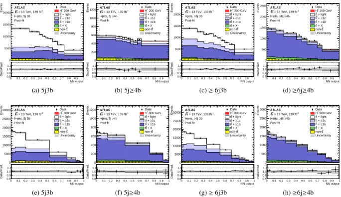
(h)≥6j≥4b, reweighted Figure 3: Comparison of the predicted leading jet𝑝
Tand data before the fit in the four analysis regions before (top) and after (bottom) the reweighting was applied. The uncertainty bands include both the statistical and systematic uncertainties. Since the normalisations of the𝑡𝑡¯+ ≥1𝑏and𝑡𝑡¯+ ≥1𝑐backgrounds are allowed to vary in the fit, no cross-section uncertainties associated with these processes are included. The lower panels display the ratio of the data to the total prediction. The hatched bands show the uncertainties before the fit to the data, which are dominated by systematic uncertainties. The𝜒2/ndf and the𝜒2 probability are also shown. Statistical uncertainties on MC predictions and data are uncorrelated across bins, while systematic uncertainties on the predictions are correlated.
•
invariant mass of the untagged jet-pair with minimum
Δ𝑅(not in 5j
≥4b),
•
average
Δ𝑅between all
𝑏-jet pairs in the event,
• Δ𝑅
between the lepton and the pair of
𝑏-jets with smallest
Δ𝑅,
•
second Fox–Wolfram moment calculated using all jets and leptons [98],
•
number of jets (only in
≥6j3b and
≥6j
≥4b regions), and
•
number of
𝑏-jets (only in 5j
≥4b and
≥6j
≥4b regions).
The variables are chosen to provide the best discrimination against the
𝑡𝑡¯
+ ≥1
𝑏background. Among them, the kinematic discriminant, scalar sum of the
𝑝T
of all jets, centrality, and leading jet
𝑝T
provide the most discrimination. The centrality is computed as the scalar sum of the
𝑝T
of all jets and leptons in the event divided by the sum of their energies. The kinematic discriminant is a variable reflecting the probability that an event is compatible with the
𝐻+→𝑡 𝑏hypothesis rather than the
𝑡𝑡¯ hypothesis, and is defined as
𝐷 =𝑃𝐻+(x)/(𝑃𝐻+(x) +𝑃𝑡¯
𝑡(x))
, where
𝑃𝐻+(x)and
𝑃𝑡¯
𝑡(x)
are probability density functions for
xunder the
signal hypothesis and background (
𝑡𝑡¯ ) hypothesis, respectively. The event variable
xindicates the set of the
missing transverse momentum and the four-momenta of the reconstructed lepton and the jets [25].
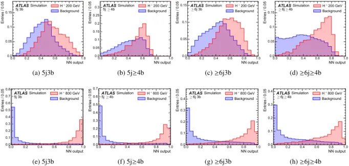
Figure 4 shows the predicted NN output distributions in the four analysis regions for selected
𝐻+signal samples and the SM background. These distributions are used in a fit to extract the amount of
𝐻+signal in data. The separation of the
𝐻+signal from the background is most difficult for low
𝐻+masses because the two processes have very similar kinematics and topology. The kinematic discriminant has large separating power at low
𝐻+masses, whereas at higher masses, where the topologies of the
𝐻+signal and the background are no longer alike, other variables, such as the scalar sum of the
𝑝T
of all jets, provide the largest separation.
0.0 0.2 0.4 0.6 0.8 1.0
NN output 0.0
0.05 0.1 0.15
Entries / 0.05
ATLAS Simulation
5j 3b H+200 GeV
Background
(a) 5j3b
0.0 0.2 0.4 0.6 0.8 1.0
NN output 0.0
0.05 0.1 0.15 0.2 0.25 0.3
Entries / 0.05
ATLAS Simulation
5j ≥4b H+200 GeV
Background
(b) 5j≥4b
0.0 0.2 0.4 0.6 0.8 1.0
NN output 0.0
0.05 0.1 0.15
Entries / 0.05
ATLAS Simulation
≥6j 3b H+200 GeV
Background
(c)≥6j3b
0.0 0.2 0.4 0.6 0.8 1.0
NN output 0.0
0.05 0.1 0.15
Entries / 0.05
ATLAS Simulation
≥6j≥4b H+200 GeV
Background
(d)≥6j≥4b
0.0 0.2 0.4 0.6 0.8 1.0
NN output 0.0
0.1 0.2 0.3 0.4 0.5 0.6 0.7 0.8
Entries / 0.05
ATLAS Simulation
5j 3b H+800 GeV
Background
(e) 5j3b
0.0 0.2 0.4 0.6 0.8 1.0
NN output 0.0
0.1 0.2 0.3 0.4 0.5 0.6 0.7
Entries / 0.05
ATLAS Simulation
5j ≥4b H+800 GeV
Background
(f) 5j≥4b
0.0 0.2 0.4 0.6 0.8 1.0
NN output 0.0
0.1 0.2 0.3 0.4
Entries / 0.05
ATLAS Simulation
≥6j 3b H+800 GeV
Background
(g)≥6j3b
0.0 0.2 0.4 0.6 0.8 1.0
NN output 0.0
0.1 0.2 0.3 0.4
Entries / 0.05
ATLAS Simulation
≥6j≥4b H+800 GeV
Background
(h)≥6j≥4b
Figure 4: Expected distributions of the NN output for𝐻+masses of 200 GeV (top) and 800 GeV (bottom) for SM backgrounds and𝐻+signal in the four analysis regions. All distributions are normalised to unity.
6 Systematic uncertainties
Various sources of experimental and theoretical uncertainties are considered in this analysis. They may affect the overall normalisation of the processes, the shapes of the NN output distributions, or both. All the experimental uncertainties considered, with the exception of that in the luminosity, affect both normalisation and shape in all the simulated samples. Uncertainties related to the modelling of the signal and background affect both normalisation and shape, with the exception of cross-section uncertainties, which only affect the normalisation of the sample considered. Nonetheless, the normalisation uncertainties modify the relative fractions of the different samples, leading to a shape variation in the final NN output distributions. A single independent nuisance parameter (NP) is assigned to each source of systematic uncertainty in the statistical analysis. Some of the systematic uncertainties, in particular most of the experimental uncertainties, are decomposed into several independent sources. Each individual source has a correlated effect across all analysis regions and signal and background samples.
The uncertainty of the integrated luminosity for the full Run-2 dataset is 1.7% [99], obtained using the
LUCID-2 detector [100] for the primary luminosity measurements. A variation in the pile-up reweighting
of the simulated events described in Section 2 is included to cover the uncertainty in the ratio of the predicted and measured inelastic cross-sections in a given fiducial volume [101].
Uncertainties associated with charged leptons arise from the trigger selection, the lepton reconstruction, identification and isolation criteria, as well as the lepton momentum scale and resolution. The reconstruction, identification and isolation efficiency of electrons and muons, as well as the efficiency of the trigger used to record the events, differ slightly between data and simulation, which is compensated for by dedicated correction factors (CFs). Efficiency CFs are measured using tag-and-probe techniques in
𝑍 → ℓ+ℓ−data and simulated samples [82, 102], and are applied to the simulation to correct for the differences.
The effect of these CFs, as well as of their uncertainties, are propagated as corrections to the MC event weight. Additional sources of uncertainty originate from the corrections applied to adjust the lepton momentum scale and resolution in the simulation to match those in data. The impact of these uncertainties on
𝜎(𝑝 𝑝 →𝑡 𝑏 𝐻+) × B (𝐻+→𝑡 𝑏)is smaller than 1%.
Uncertainties associated with jets arise from the efficiency of pile-up rejection by the JVT, from the jet energy scale (JES) and resolution (JER), and from
𝑏-tagging. Correction factors are applied to correct for differences between data and MC simulation for JVT efficiencies. These CFs are estimated using
𝑍(→ 𝜇+𝜇−)+ jets with tag-and-probe techniques similar to those in Ref. [87]. The JES and its uncertainty are derived by combining information from test-beam data, collision data and simulation [85].
Additional uncertainties are considered, related to jet flavour, quark/gluon fraction, pile-up corrections,
𝜂dependence, high-
𝑝T
jets, and differences between full and fast simulation. The JER uncertainty is obtained by combining dijet balance measurements in data and simulation [103]. The
𝑏-tagging efficiencies in simulated samples are corrected to match efficiencies in data. Correction factors are derived as a function of
𝑝T
for
𝑏-,
𝑐- and light-jets separately in dedicated calibration analyses. For
𝑏-jet efficiencies,
𝑡𝑡¯ events in the di-lepton topology are used, exploiting the very pure sample of
𝑏-jets arising from the decays of the top quarks [89]. For
𝑐-jet mistag rates,
𝑡𝑡¯ events in single-lepton topology are used, exploiting the
𝑐-jets from the hadronically decaying
𝑊bosons, using techniques similar to those in Ref. [104]. For light-jet mistag rates, the so-called negative-tag method similar to that in Ref. [105] is used, but using
𝑍+jets events instead of di-jet events.
All the uncertainties described above on energy scales or resolutions of the reconstructed objects are propagated to the missing transverse momentum. Additional uncertainties in the scale and resolution of the soft term are considered, which account for the disagreement between data and simulation of the
𝑝T
balance between the hard and the soft components. A total of three independent sources are added: an offset along the hard component
𝑝T
axis, and the smearing resolution along and perpendicular to this axis [106, 107]. Since the missing transverse momentum is not used in selection but only in the event reconstruction, the associated uncertainties have an impact smaller than 1%.
The uncertainty in the
𝐻+signal due to different scale choices is estimated by varying
𝜇f
and
𝜇r
up and down by a factor of two. The uncertainties from the modelling of the PDF are evaluated replacing the nominal NNPDF2.3NLO PDF set by a symmetrised Hessian set, PDF4LHC15_nlo_30, following the PDF4LHC recommendations for LHC Run 2 [108].
The modelling of the
𝑡𝑡¯ + jets background is one of the largest sources of uncertainty in the analysis, and several different components are considered. The 6% uncertainty for the inclusive
𝑡𝑡¯ production cross-section predicted at NNLO+NNLL includes effects from varying
𝜇f
and
𝜇r
, the PDF,
𝛼S
, and the
top-quark mass [109]. This uncertainty is applied to
𝑡𝑡¯ + light only, since the normalisation of
𝑡𝑡¯
+ ≥1
𝑏and
𝑡𝑡¯
+ ≥1
𝑐are allowed to vary freely in the fit. Besides normalisation, the
𝑡𝑡¯
+light,
𝑡𝑡¯
+ ≥1
𝑏and
𝑡𝑡¯
+ ≥1
𝑐processes are affected by different types of uncertainties: the uncertainties associated with additional
Feynman diagrams for the
𝑡𝑡¯
+light are constrained from relatively precise measurements in data [110];
𝑡𝑡
¯
+ ≥1
𝑏and
𝑡𝑡¯
+ ≥1
𝑐can have similar or different Feynman diagrams depending on the flavour scheme used for the PDF, and the different masses of the
𝑏- and the
𝑐-quarks contribute to additional differences between these two processes. For these reasons, all uncertainties in the
𝑡𝑡¯ + jets background modelling are assigned independent NP for
𝑡𝑡¯
+light,
𝑡𝑡¯
+ ≥1
𝑏and
𝑡𝑡¯
+ ≥1
𝑐. Systematic uncertainties in the acceptance and shapes are extracted by comparing the nominal prediction with alternative MC samples or settings.
Such comparisons would significantly change the fractions of
𝑡𝑡¯
+ ≥1
𝑏and
𝑡𝑡¯
+ ≥1
𝑐. However, since the normalisation of these sub-processes in the analysis regions is determined in the fit, these alternative predictions are reweighted in such a way that they keep the same fractions of
𝑡𝑡¯
+ ≥1
𝑏and
𝑡𝑡¯
+ ≥1
𝑐as the nominal sample in the phase-space selected by the analysis.
The uncertainty due to initial state radiation (ISR) is estimated by using the Var3cUp (Var3cDown) variant from the A14 tune [48], corresponding to
𝛼ISRS =
0.140 (0.115) instead of the nominal
𝛼ISRS =
0
.127.
Uncertainties related to
𝜇f
and
𝜇r
are estimated by scaling each one up and down by a factor of two. For the final state radiation (FSR), the amount of radiation is increased (decreased) in the PS corresponding to
𝛼FSRS =
0.142 (0.115) instead of the nominal
𝛼FSRS =
0
.127. The nominal PowhegBox+Pythia sample is compared with the PowhegBox+Herwig sample to assess the effect of the PS and hadronisation models, and to the MadGraph5_aMC@NLO sample to assess the effect of the NLO matching technique. The nominal PowhegBox+Pythia 5FS prediction for the dominant
𝑡𝑡¯
+ ≥1
𝑏background, in which all the additional partons are produced by the PS, is compared with an alternative PowhegBox+Pythia 4FS sample, in which the
𝑏𝑏¯ pair is generated in addition to the
𝑡𝑡¯ pair at the ME level. An uncertainty resulting from the comparison of the shapes of the two models is included. Finally, the weights derived in Section 4 to improve the agreement of the simulation with data are varied within their statistical uncertainties, in a correlated way among the three
𝑡𝑡¯ + jets components. All the sources of systematic uncertainty for the
𝑡𝑡¯ + jets modelling are summarised in Table 2.
Table 2: Summary of the sources of systematic uncertainty for𝑡¯𝑡+ jets modelling. The systematic uncertainties listed in the second section of the table are evaluated in such a way as to have no impact on the normalisation of the three, 𝑡𝑡¯+ ≥1𝑏,𝑡𝑡¯+ ≥1𝑐and𝑡𝑡¯+light, components in the phase-space selected in the analysis. The last column of the table indicates the𝑡𝑡¯+ jets components to which the systematic uncertainty is assigned. All systematic uncertainty sources, except those associated to the𝑡𝑡¯reweighting, are treated as uncorrelated across the three components.
Uncertainty source Description Components
𝑡𝑡¯cross-section Up or down by 6% 𝑡𝑡¯+light
𝑡𝑡¯reweighting Statistical uncertainties of fitted function (six) parameters All𝑡𝑡¯and𝑊 𝑡
𝑡𝑡¯+ ≥1𝑏modelling 4FS vs 5FS 𝑡𝑡¯+ ≥1𝑏
𝑡𝑡¯+ ≥1𝑏normalisation Free-floating 𝑡𝑡¯+ ≥1𝑏
𝑡𝑡¯+ ≥1𝑐normalisation Free-floating 𝑡𝑡¯+ ≥1𝑐
NLO matching MadGraph5_aMC@NLO+Pythia vs PowhegBox+Pythia All𝑡𝑡¯ PS & hadronisation PowhegBox+Herwig vs PowhegBox+Pythia All𝑡𝑡¯
ISR Varying𝛼ISR
S in PowhegBox+Pythia All𝑡𝑡¯
𝜇f Scaling by 0.5 (2.0) in PowhegBox+Pythia All𝑡𝑡¯
𝜇r Scaling by 0.5 (2.0) in PowhegBox+Pythia All𝑡𝑡¯
FSR Varying𝛼FSR
S in PowhegBox+Pythia All𝑡𝑡¯
A 5% uncertainty is considered for the cross-sections of the three single-top production modes [111–115].
Uncertainties associated with the PS and hadronisation model, and with the NLO matching scheme
are evaluated by comparing, for each process, the nominal PowhegBox+Pythia sample with a sample
produced using PowhegBox+Herwig [116] and MadGraph5_aMC@NLO+Pythia, respectively. As mentioned in Section 4, the
𝑊 𝑡single-top mode is included in the reweighting procedure, and thus the same uncertainties used for
𝑡𝑡¯ are applied here. The uncertainty associated to the interference between
𝑊 𝑡and
𝑡𝑡¯ production at NLO [63] is assessed by comparing the nominal PowhegBox+Pythia sample produced using the “diagram removal” scheme with an alternative sample produced with the same generator but using the “diagram subtraction” scheme [62, 63].
The predicted SM
𝑡𝑡 𝐻¯ signal cross-section uncertainty is
+−59..8%2%(QCD scale)
±3
.6% (PDF +
𝛼S
) [13, 117–121]. Uncertainties of the Higgs boson branching ratios amount to 2.2% for the
𝑏𝑏¯ decay mode [13].
For the ISR and FSR, the amount of radiation is varied following the same procedure as for
𝑡𝑡¯ . The nominal PowhegBox+Pythia sample is compared with the PowhegBox+Herwig sample to assess the uncertainty due to PS and hadronisation, and to the MadGraph5_aMC@NLO sample for the uncertainty due to the NLO matching.
The uncertainty of the
𝑡𝑡𝑉¯ NLO cross-section prediction is 15%, split into PDF and scale uncertainties as for
𝑡𝑡 𝐻¯ [13, 122]. An additional
𝑡𝑡𝑉¯ modelling uncertainty, related to the choice of PS and hadronisation model and matching scheme, is assessed by comparing the nominal MadGraph5_aMC@NLO+Pythia samples with alternative samples generated with Sherpa.
An overall 50% normalisation uncertainty is considered for the four-top-quarks background, covering effects from varying
𝜇f
,
𝜇r
, PDF and
𝛼S
[45, 123]. The small background
𝑡 𝑍 𝑞is assigned a 7.9% and a 0.9% uncertainty accounting for
𝜇f
and
𝜇r
scales and PDF variations, respectively. Finally, a single 50%
uncertainty is used for
𝑡 𝑍 𝑊[45].
An uncertainty of 40% is assumed for the
𝑊+jets normalisation, with an additional 30% for
𝑊+ heavy- flavour jets, taken as uncorrelated between events with two and more than two heavy-flavour jets. These uncertainties are based on variations of the
𝜇f
and
𝜇r