SFB 649 Discussion Paper 2005-020
A Dynamic
Semiparametric Factor Model for Implied
Volatility String Dynamics
Matthias R. Fengler*
Wolfgang K. Härdle**
Enno Mammen***
* Trading & Derivatives, Sal. Oppenheim jr. & Cie., Germany
** CASE – Center for Applied Statistics and Economics, Humboldt-Universität zu Berlin, Germany
*** Department of Economics, University of Mannheim, Germany
This research was supported by the Deutsche
Forschungsgemeinschaft through the SFB 649 "Economic Risk".
http://sfb649.wiwi.hu-berlin.de ISSN 1860-5664
SFB 649, Humboldt-Universität zu Berlin
S FB
6 4 9
E C O N O M I C
R I S K
B E R L I N
A Dynamic Semiparametric Factor Model for Implied Volatility String Dynamics ∗
Matthias R. Fengler
†Trading & Derivatives, Sal. Oppenheim jr. & Cie.
Untermainanlage 1, 60329 Frankfurt am Main, Germany
Wolfgang K. H¨ ardle
CASE – Center for Applied Statistics and Economics Humboldt-Universit¨at zu Berlin,
Spandauer Straße 1, 10178 Berlin, Germany
Enno Mammen
Department of Economics, University of Mannheim L 7, 3–5, 68131 Mannheim, Germany
March 6, 2005
∗We gratefully acknowledge financial support by the Deutsche Forschungsgemeinschaft and the Sonder- forschungsbereich 649 “ ¨Okonomisches Risiko”.
†Corresponding author: matthias.fengler@oppenheim.de, TEL ++49 69 7134 5512, FAX ++49 69 7134 9 5512. The paper represents the author’s personal opinion and does not reflect the views of Sal. Oppenheim.
A Dynamic Semiparametric Factor Model for Implied Volatility String Dynamics
Abstract
A primary goal in modelling the implied volatility surface (IVS) for pricing and hedging aims at reducing complexity. For this purpose one fits the IVS each day and applies a principal component analysis using a functional norm. This approach, however, neglects the degenerated string structure of the implied volatility data and may result in a modelling bias. We propose a dynamic semiparametric factor model (DSFM), which approximates the IVS in a finite dimensional function space. The key feature is that we only fit in the local neighborhood of the design points. Our approach is a combination of methods from functional principal component analysis and backfitting techniques for additive models. The model is found to have an approximate 10% better performance than a sticky moneyness model. Finally, based on the DSFM, we devise a generalized vega-hedging strategy for exotic options that are priced in the local volatility framework. The generalized vega-hedging extends the usual approaches employed in the local volatility framework.
JEL classification codes: C14, G12
Keywords: smile, local volatility, generalized additive model, backfitting, functional principal component analysis
1 Introduction
Successful trading, hedging and risk managing of option portfolios crucially depends on the accuracy of the underlying pricing models. Consequently, new valuation approaches are continuously developed in departing from the foundations of option theory laid by Black and Scholes (1973), Merton(1973) and Harrison and Kreps(1979), and existing models are refined. However, despite these pervasive developments, the model of Black and Scholes (1973) remains a pivot in modern financial theory and an important benchmark for more sophisticated models, be it from a theoretical or practical point of view.
The popularity of the Black and Scholes (BS) model is likely due to its clear and easy-to- communicate set of assumptions. Based on the geometric Brownian motion for the under- lying asset price dynamics, and continuous trading in a complete and frictionless market, simple closed form solutions for plain vanilla calls and puts are derived: given the current un- derlying price at time, the option’s strike price, its expiry date the prevailing riskless interest rate, and an estimate of the (expected) market volatility, option prices are straightforward to compute.
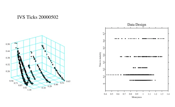
The crucial parameter in option valuation by BS is the market volatility. Since it is unknown, one studiesimpliedvolatility, which is derived by inverting the BS formula for a cross section of options with different strikes and maturities traded at the same point in time. As is visible in the left panel of Figure 1 for May 2, 2000 (i.e. 20000502, a notation we will use from now on), implied volatilities display a remarkable curvature across the strike dimension, and – albeit to a lesser degree – a term structure across time to maturity. For a given time to maturity the phenomenon is called smile or smirk. This dependence given by the mapping ˆ
σt : (κ, τ)→σˆt(κ, τ), where κdenotes the strike dimension scaled in moneyness and τ time to maturity, is called implied volatility surface (IVS). The indext denotes time-dependence.
Apparently, it is in contrast with the BS framework in which volatility is assumed to be a constant across strikes, time to maturity and also time.
There is a considerable amount of literature which aims at reconciling this empirical antag- onism with financial theory. Generally speaking, this can be achieved by including another degree of freedom into option pricing models: well-known examples are stochastic volatility
IVS Ticks 20000502
0.16 0.28 0.40 0.51 0.63 0.56
0.71 0.87
1.02 1.18 0.26
0.32 0.38 0.44 0.50
Data Design
0.4 0.5 0.6 0.7 0.8 0.9 1 1.1 1.2 1.3 1.4
Moneyness
00.10.20.30.40.50.60.7
Time to maturity
Figure 1: Left panel: call and put implied volatilities observed on 2nd May, 2000. Right panel: data design on 2nd May, 2000, ODAX. Lower left axis is moneyness κ def= K/Ft, where Ft denotes the futures price, lower right axis time to maturity
models (Hull and White, 1987; Stein and Stein, 1991; Heston, 1993), models with jump diffusions (Bates,1996a,b), or models building on general L´evy processes, e.g. based on the inverse Gaussian (Barndorff-Nielsen, 1997), and generalized hyperbolic distribution (Eber- lein and Prause,2002). These approaches capture the smile and term structure phenomena and the complexity of its dynamics to some extent, as is documented for instance in Das and Sundaram (1999) and Bergomi (2004).
Nevertheless, the BS model and the IVS enjoy much popularity. Partly, this is due to the fact that the IVS is derived from a cross-section of option prices at a specific point in time.
Therefore, unlike estimates based on historical data, the IVS is a widely accepted state variable that reflects current market sentiments, Bakshi et al. (2000). More importantly, however, the IVS plays a decisive role in trading: market makers at plain vanilla desks con- tinuously monitor and update the IVS they trade on; and exotic derivatives trader calibrate their pricing engines with an estimate of the IVS. This is particularly obvious for the pricing systems relying on the local volatility models. Initially developed byDupire (1994) andDer-
Model fit 20000502
0.14 0.23 0.32 0.41 0.50 0.80
0.88 0.96
1.04 1.12 -1.46
-1.30 -1.14 -0.98 -0.82
Semiparametric factor model fit 20000502
0.14 0.23 0.32 0.41 0.50 0.80
0.88 0.96
1.04 1.12 -1.47
-1.31 -1.16 -1.00 -0.85
Figure 2: Nadaraya-Watson estimator and DSFM fit for 20000502. Bandwidths for both estimates h1 = 0.03 for the moneyness and h2 = 0.04 for the time to maturity dimension.
Axes as in the left panel.
man and Kani (1994), they are in wide-spread use in form of the efficient implementations by Andersen and Brotherton-Ratcliffe (1997) and Dempster and Richards (2000). Thus, refined statistical model building of the IVS determines vitally the accuracy of applications in trading and risk-management.
In modelling the IVS one faces two main challenges. First, the data have a degenerated design: due to institutional conventions, observations of the IVS occur only for a small number of maturities such as one, two, three, six, nine, twelve, 18, and 24 months to expiry on the date of issue. Consequently, implied volatilities appear in a row like pearls strung on a necklace, Figure 1, or, in short: as ‘strings’. This pattern is visible in the right panel of Figure 1, which plots the data design as seen from top. Options belonging to the same string have a common time to maturity. As time passes, the strings move through the maturity axis towards expiry while changing levels and shape in a random fashion. Second, also in the moneyness dimension, the observation grid does not cover the desired estimation grid at any point in time. Thus, even when the data sets are huge, for a large number of cases implied volatility observations are missing for certain sub-regions of the desired estimation
grid. This is particularly virulent when transaction based data are used. However, despite their appearance as strings, implied volatilities are thought as being the observed structure of a smooth surface. This is because in practice one needs to price and hedge OTC options whose expiry dates do not coincide with the expiry dates of the options that are traded at the futures exchange.
For the semi- or nonparametric approximations to the IVS that have been promoted byA¨ıt- Sahalia and Lo (1998), Rosenberg (2000), A¨ıt-Sahalia et al. (2001b), Cont and da Fonseca (2002),Fengler et al.(2003) and Fengler and Wang(2003), this design may pose difficulties.
For illustration, consider in Figure 2 (left panel) the fit of a standard Nadaraya-Watson estimator. Bandwidths are h1 = 0.03 for the moneyness and h2 = 0.04 for the time to maturity dimension (measured in years). The fit appears very rough, and there are huge holes in the surface, since the bandwidths are too small to ‘bridge’ the gaps between the maturity strings. In order to remedy this deficiency one would need to strongly increase the bandwidths which may induce a large bias. Moreover, since the design is time-varying, the bandwidths would also need to be adjusted anew for each trading day, which complicates daily applications. Parametric models, e.g. as inShimko(1993),An´e and Geman(1999), and Brockhaus et al. (2000, Chap. 2) among others, are less affected by these data limitations, but appear to offer too little functional flexibility to capture the salient features of IVS patterns. Thus, parametric estimates may as well be biased.
In this paper we provide a new principal component approach for modelling the IVS: the complex dynamic structure of the IVS is captured by a low-dimensional dynamic semipara- metric factor model (DSFM) with time-varying coefficients. The IVS is approximated by unknown basis functions moving in a finite dimensional function space. The dynamics can be understood by using vector autoregression (VAR) techniques on the time-varying co- efficients. Contrary to earlier studies, we will use only finite dimensional fits to implied volatilities which are obtained in the local neighborhood of strikes and maturities, for which implied volatilities are recorded at the specific day. Surface estimationanddimension reduc- tion is achieved in one single step. Our technology can be seen as a combination of functional principal component analysis, nonparametric curve estimation and backfitting for additive models.
Intuitively, the localization of our methodology can be interpreted as smoothing through
time, i.e. for fitting, the information contained in other observations dates in the sample is exploited, see Section 2 for the details. This is possible due to the expiry effect which is a unique feature present IVS data. As explained, this effect insures that observations gradually move through the entire observation space. To our knowledge there do not exist estimation techniques that explicitly take advantage of this effect.
To introduce our model, let us denote the implied volatility by Yi,j, where the index i is the number of the day (i = 1, . . . , I), and j = 1, . . . , Ji is an intra-day numbering of the option traded on day i. The observations Yi,j are regressed on two-dimensional covariables Xi,j that contain moneynessκi,j and maturityτi,j. Moneyness is defined asκi,j def= Ki,j/Ft,i,j, i.e. strike Ki,j divided by the underlying futures price Ft,i,j at timeti,j. We also considered the one-dimensional case in which Xi,j =κi,j. However, since modelling the entire surface is more interesting, we will present results for this case only. The DSFM is given by:
m0(Xi,j) +
L
X
l=1
βi,lml(Xi,j), (1)
where ml are smooth basis functions (l = 0, . . . , L). The IVS is approximated by a weighted sum of smooth functions ml with weights βi,l depending on time i. The factor loading βi def= (βi,1, . . . βi,L)> forms an unobserved multivariate time series. By fitting model (1), to the implied volatility strings we obtain approximations βbi. We argue that the VAR estimation based on βbi is asymptotically equivalent to estimation based on the unobserved βi. A justification for this is given in Borak et al. (2005) where the relations to Kalman filtering are discussed.
Lower dimensional approximations of the IVS based on principal components analysis (PCA) have been used in Zhu and Avellaneda (1997) andFengler et al. (2002) in an application to the term structure of implied volatilities, and in Skiadopoulos et al. (1999) and Alexander (2001) in studies across strikes. Fengler et al. (2003) use a common principal components approach to study several maturity groups across the IVS simultaneously, while Cont and da Fonseca (2002) propose a functional PCA perspective for the IVS. All these approaches treat the IVS as a stationary process, and do not take particular care for the degenerated string structure apparent in Figure 1.
Our modelling approach is also different in the following respect: for instance, in Cont and da Fonseca (2002) the IVS is fitted on a grid for each day. Afterwards a PCA using a functional norm is applied to the surfaces. This treatment follows the usual functional PCA approach as described in Ramsay and Silverman (1997). In our approach the IVS is fitted each day at the observed design points Xi,j. This leads to a minimization with respect to functional norms that depend on timei. We loose a nice feature of the usual functional PCA though: when fitting the data forLand L∗ =L+ 1, the linear space spanned bymb0, . . . ,mbL may not be contained in the one spanned by mb∗0, . . . ,mb∗L∗. On the other hand we only make use of values of the implied volatilities at regions where they are observed. This avoids bias effects caused by global daily fits used in standard functional PCAs.
The model can be employed in several respects: given the estimated functions mbl and the time series β, scenario simulations of potential IVS scenarios are straightforward. They canb help to give a more accurate assessment of market risk than previous approaches. Worst case scenarios can be identified, which provide additional supervision tools to risk managers. For trading, the model may be used as a tool of short range IVS prediction or as an input factor in the local volatility models such as the one by Andersen and Brotherton-Ratcliffe(1997).
As we will demonstrate, the model also offers a unified tool to traders for vega hedging of complex option positions in a local volatility setting.
The paper is organized as follows: in the following section, implied volatilities are described and the DSFM is introduced. In Section 3 the model is applied to DAX option implied volatilities for the sample period 1998 to May 2001. Section 4 discusses the hedging of complex option positions in the local volatility setting, Section 5 concludes.
2 Time-dependent implied volatility modelling
2.1 The semiparametric factor model
Implied volatilities are derived from the BS option pricing formula for European calls and puts, Black and Scholes (1973). European style calls and puts are contingent claims on an asset St (paying no dividends for simplicity, here), which yield the pay-off max(St−K,0)
and max(K −St,0), respectively, for a strike K at a given expiry day T. The asset price process St in the BS model is assumed to be a geometric Brownian motion. The BS option pricing formula for calls is given by:
CtBS(St, K, τ, r, σ) = StΦ(d1)−e−rτKΦ(d2), (2) where d1 def= log(St/K)+(r+σ√τ 12σ2)τ and d2 def= d1−σ√
τ. Φ(·) denotes the cumulative distribution function of the standard normal distribution, τ def= T −t time to maturity of the option, r the riskless interest rate over the option’s life time, and σ the diffusion coefficient of the Brownian motion. Put prices Pt are obtained via the put-call-parityCt−Pt =St−e−τ rK.
The only unknown parameter in (2) is the volatility parameter σ. Given observed market prices ˜Ct, implied volatility ˆσ is defined by:
CtBS(St, K, τ, r,σ)ˆ −C˜t= 0 . (3) Due to monotonicity of the BS price in σ, there exists a unique solution ˆσ >0. Define the moneyness metric κtdef= K/Ft, where Ft denotes the futures price time t.
In the dynamic factor model, we regress Yi,j
def= log{ˆσi,j(κ, τ)} on Xi,j = (κi,j, τi,j) via nonparametric methods. We work with log-implied volatility data, since the data appear less skewed and potential outliers are scaled down after taking logs. This is common practice in the IVS literature, see e.g. Zhu and Avellaneda (1997) and Cont and da Fonseca (2002).
In order to estimate the nonparametric componentsmland the state variables βi,l in (1), we borrow ideas from fitting additive models as in Stone (1986), Hastie and Tibshirani (1990) and Horowitz et al. (2002). Our research is related to functional coefficient models such as Cai et al. (2000). Other semi- and nonparametric factor models include Connor and Linton (2000), Gouri´eroux and Jasiak (2001), Fan et al. (2003), and Linton et al. (2003).
Nonparametric techniques are now broadly used in option pricing, e.g. Broadie et al.(2000a), Broadie et al. (2000b), A¨ıt-Sahalia et al. (2001a), and A¨ıt-Sahalia and Duarte (2003).
The estimatesmbl, (l = 0, . . . , L) andβbi,l(i= 1, . . . , I; l= 1, . . . , L) are defined as minimizers of the following least squares criterion (βbi,0
def= 1):
I
X
i=1 Ji
X
j=1
Z ( Yi,j−
L
X
l=0
βbi,lmbl(u) )2
Kh(u−Xi,j) du . (4)
Here, Kh denotes a two-dimensional product kernel,Kh(u) =kh1(u1)×kh2(u2), h= (h1, h2), based on a one-dimensional kernel kh(v)def= h−1k(h−1v).
In (4) the minimization runs over all functions mbl : R2 → R and all values βbi,l ∈ R. For illustration let us consider the case L = 0 : implied volatilities Yi,j are approximated by a surface mb0 that does not depend on time i. In this degenerated case, mb0(u) =P
i,jKh(u− Xi,j)Yi,j/P
i,jKh(u−Xi,j), which is the Nadaraya-Watson estimate based on the pooled sample of all days.
Using (4), the implied volatility surfaces are approximated by surfaces moving in an L- dimensional affine function space {mb0+PL
l=1αlmbl: α1, . . . , αL∈R}.The estimates mbl are not uniquely defined: they can be replaced by functions that span the same affine space.
In order to respond to this problem, we select mbl such that they are orthogonal. This will facilitate the interpretation of the functions, as shall be seen in Section 3 and 4.
Replacing in (4)mblbymbl+δgwith arbitrary functionsg and taking derivatives with respect to δ yields, for 0≤l0 ≤L:
I
X
i=1 Ji
X
j=1
( Yi,j−
L
X
l=0
βbi,lmbl(u) )
βbi,l0Kh(u−Xi,j) = 0. (5) Furthermore, by replacing βbi,l by βbi,l+δ in (4) and again taking derivatives with respect to δ, we get for 1 ≤l0 ≤L and 1≤i≤I:
Ji
X
j=1
Z ( Yi,j−
L
X
l=0
βbi,lmbl(u) )
mbl0(u)Kh(u−Xi,j) du= 0. (6) Introducing the following notation, for 1 ≤i≤I
pbi(u) = 1 Ji
Ji
X
j=1
Kh(u−Xi,j), (7)
qbi(u) = 1 Ji
Ji
X
j=1
Kh(u−Xi,j)Yi,j , (8)
we obtain from (5)-(6), for 1≤l0 ≤L,1≤i≤I:
I
X
i=1
Jiβbi,l0qbi(u) =
I
X
i=1
Ji
L
X
l=0
βbi,l0βbi,lpbi(u)mbl(u), (9) Z
bqi(u)mbl0(u) du =
L
X
l=0
βbi,l Z
pbi(u)mbl0(u)mbl(u) du . (10)
We calculate the estimates by iterative use of (9) and (10). We start by initial valuesβbi,l(0) for βbi,l. A possible choice of the initial βbcould correspond to fits of surfaces that are piecewise constant on time intervals I1, . . . , IL. This means, for l = 1, .., L, put βbi,l(0) = 1 (for i ∈ Il), and βbi,l(0) = 0 (for i /∈ Il). Here I1, ..., IL are pairwise disjoint subsets of {1, ..., I} and
L
S
l=1
Il
is a strict subset of {1, ..., I}. For r ≥0, we put βbi,0(r) = 1. Define the matrix B(r)(u) by its elements:
B(r)(u)
l,l0 def=
I
X
i=1
Jiβbi,l(r−1)0 βbi,l(r−1)bpi(u), 0≤l, l0 ≤L , (11) and introduce a vector Q(r)(u) with elements
Q(r)(u)l def=
I
X
i=1
Jiβbi,l(r−1)qbi(u), 0≤l ≤L . (12) In the r-th iteration the estimate mb = (mb0, . . . ,mbL)> is given by:
mb(r)(u) =B(r)(u)−1Q(r)(u). (13) This update step is motivated by (9). The values of βb are updated in the r-th cycle as follows: define the matrix M(r)(i)
M(r)(i)
l,l0 def=
Z
pbi(u)mb(r)l0 (u)mb(r)l (u)du , 1≤l, l0 ≤L , (14) and define a vector S(r)(i)
S(r)(i)ldef= Z
qbi(u)mbl(u) du− Z
pbi(u)mb(r)0 (u)mb(r)l (u) du , 1≤l ≤L . (15) Motivated by (10), put
βbi,1(r), ...,βbi,L(r)>
=M(r)(i)−1S(r)(i). (16)
The algorithm is run until only minor changes occur. In the implementation, we choose a grid of points and calculate mbl at these points. In the calculation of M(r)(i) and S(r)(i), we replace the integral by a Riemann sum approximation using the values of the integrated functions at the grid points.
As discussed above, mbl and βbi,l are not uniquely defined. Therefore, we orthogonolize mb0, . . . ,mbL in L2(ˆp), where ˆp(u) = I−1PI
i=1pˆi(u), such that PI
i=1βbi,12 is maximal, and given βbi,1,mb0,mb1, PI
i=1βbi,22 is maximal, and so forth. These aims can be achieved by the following two steps: first replace
mb0 by mbnew0 = mb0−γ>Γ−1m ,b mb by mbnew = Γ−1/2m ,b
βbi,1
... βbi,L
by
βbi,1new
... βbi,Lnew
= Γ1/2
βbi,1
... βbi,L
+ Γ−1γ
,
(17)
where mb = (mb1, . . . ,mbL)> and the (L×L) matrix Γ = R
m(u)b m(u)b >p(u)ˆ du, or for clar- ity, Γ = (Γl,l0), with Γl,l0 = R
mbl(u) mbl0(u)ˆp(u)du. Finally, we have γ = (γl), with γl = R
mb0(u)mbl(u)ˆp(u)du.
Note that by applying (17), mb0 is replaced by a function that minimizes R
mb20(u)ˆp(u)du.
This is evident because mb0 is orthogonal to the linear space spanned by mb1, . . .mbL. By the second equation of (17), mb1, . . . ,mbL are replaced by orthonormal functions in L2(ˆp).
In a second step, we proceed as in PCA and define a matrix B with Bl,l0 =PI
i=1βbi,lβbi,l0 and calculate the eigenvalues of B, λ1 > . . . > λL, and the corresponding eigenvectors z1, . . . zL. Put Z = (z1, . . . , zL). Replace
mb by mbnew = Z>m ,b (18) (i.e. mbnewl =zl>m),b and
βbi,1
... βbi,L
by
βbi,1new
... βbi,Lnew
= Z>
βbi,1
... βbi,L
. (19)
After application of (18) and (19) the orthonormal basis mb1, . . . ,mbL is chosen such that PI
i=1βb2i,1 is maximal, and – given βbi,1,mb0,mb1 – the quantity PI
i=1βbi,22 is maximal, . . ., i.e.
mb1 is chosen such that as much as possible is explained by βbi,1mb1. Next mb2 is chosen to achieve maximum explanation by βbi,1mb1+βbi,2mb2, and so forth.
The functions mbl are not eigenfunctions of an operator as in usual functional PCA. This is because we use a different norm, namely R
f2(u)ˆpi(u)du, for each day. Through the norming procedure the functions are chosen as eigenfunctions in an L-dimensional approximating lin- ear space. The L-dimensional approximating spaces are not necessarily nested for increasing L. For this reason the estimates cannot be calculated by an iterative procedure that starts by fitting a model with one component, and that uses the old L−1 components in the iteration step from L−1 toLto fit the next component. The calculation of mb0, . . . ,mbLhas to be fully redone for different choices of L.
3 The dynamic factors of the DAX index IVS
3.1 Data description and preparation
Our data set contains tick statistics on DAX futures contracts and DAX index options traded at the futures exchange EUREX in Frankfurt/Main in the period from January 1998 to May 2001. Both futures price and option price data are contract based data, i.e. each single contract is registered together with its price, contract size, and time of settlement up to a hundredth second. Interest rate data in daily frequency, i.e. one-, three-, six-, and twelve-months FIBOR rates for the years 1998–1999 and EURIBOR rates for the period 2000–2001, were obtained from Thomson Financial Datastream. Interest rate data were linearly interpolated to approximate the riskless interest rate for the option specific time to maturity.
In a first step, we recover the DAX index values. To this end, we group to each option price observation the futures price Ft of the nearest available futures contract, which was traded within a one minute interval around the observed option. The futures price observation was taken from the most heavily traded futures contract on the particular day, usually the three-
Min. Max. Mean Median Stdd. Skewn. Kurt.
All Time to maturity 0.028 2.014 0.131 0.083 0.148 3.723 23.373 Moneyness 0.325 1.856 0.985 0.993 0.098 -0.256 5.884 Implied volatility 0.041 0.799 0.279 0.256 0.090 1.542 6.000 1998 Time to maturity 0.028 2.014 0.134 0.081 0.148 3.548 22.957 Moneyness 0.386 1.856 0.984 0.992 0.108 -0.030 5.344 Implied volatility 0.041 0.799 0.335 0.306 0.114 0.970 3.471 1999 Time to maturity 0.028 1.994 0.126 0.083 0.139 4.331 32.578 Moneyness 0.371 1.516 0.979 0.992 0.099 -0.595 5.563 Implied volatility 0.047 0.798 0.273 0.259 0.076 0.942 4.075 2000 Time to maturity 0.028 1.994 0.130 0.083 0.151 3.858 23.393 Moneyness 0.325 1.611 0.985 0.992 0.092 -0.337 6.197 Implied volatility 0.041 0.798 0.254 0.242 0.060 1.463 7.313 2001 Time to maturity 0.028 0.978 0.142 0.083 0.159 2.699 10.443 Moneyness 0.583 1.811 1.001 1.001 0.085 0.519 6.762 Implied volatility 0.043 0.789 0.230 0.221 0.049 1.558 7.733 Table 1: Summary statistics on the data base from 199801 to 200105 for the IVS application in Section 3.2, entirely and on an annual basis. 2001 is from 200101 to 200105, only.
months contract. The no-arbitrage price of the underlying index in a frictionless market without dividends is given by St=Fte−rTF ,t(TF−t), whereSt andFt denote the index and the futures price respectively, TF the futures contract’s maturity date, andrT,t the interest rate with maturity T −t.
The DAX index is a capital weighted performance index, i.e. dividends less corporate tax are reinvested into the index, Deutsche B¨orse (2002). Therefore, dividend payments should have no impact on index options. However, when only the interest rate discounted futures price is used to recover implied volatilities by inverting the BS formula, implied volatilities of calls and puts can differ significantly. To accommodate for this fact we apply a correction algorithm that is described in Appendix B. The entire data set is stored in the financial database MD*base, www.mdtech.de, maintained at the Center for Applied Statistics and Economics (CASE), Berlin.
Since the data are transaction based and may contain misprints or outliers, a filter is applied before estimating the model: observations with implied volatility less than 4% and bigger than 80% are dropped. Furthermore, we disregard all observations having a maturity less than ten days. After this filtering, the entire number of observations is more than 4.48 million contracts, i.e. is around 5 200 observations per day.
Table 1 gives a short summary of our IVS data. Most heavy trading occurs in short term contracts, as is seen from the difference between median and mean of the term structure distribution of observations as well as from its skewness. Median time to maturity is 30 days (0.083 years). Across moneyness the distribution is slightly negatively skewed. Mean implied volatility over the sample period is 27.9%.
3.2 Empirical evidence
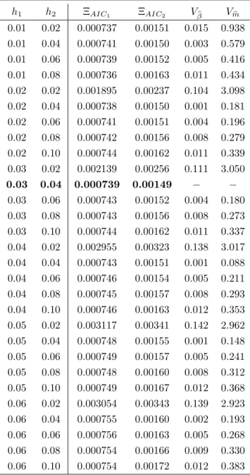
We model log-implied volatility Yi,j on Xi,j = (κi,j, τi,j)>. The grid covers in moneyness κ ∈ [0.80,1.20] and in time to maturity τ ∈ [0.05,0.5] measured in years. We employ L = 3 basis functions, which capture around 96.0% of the variations in the IVS. To our understanding, this is of sufficiently high accuracy. The bandwidths are h1 = 0.03 for moneyness and h2 = 0.04 for time to maturity. This choice is justified by Table 3.2 which presents the estimates for the two Akaike information criteria (AIC) that are explained in detail in AppendixA. Both criterion functions become very flat near the minimum. Criterion ΞAIC2 assumes its global minimum in the neighborhood of h∗ = (0.03,0.04)>, which is why we opt for these bandwidths. In being able to choose these small bandwidths, the strength of our modelling approach is demonstrated: indeed, the bandwidth in the time to maturity dimension is so small that in a fit of a particular day, data belonging to contracts with two adjacent time to maturities do not enter together pbi(u) in (7) andqbi(u) in (8). In fact, for a given u0, the quantitiespbi(u0) andqbi(u0) are zero most of the time, and only assume positive values for dates i, when observations are in the local neighborhood ofu0. Of course, during the entire observation period I, it is mandatory that observations for eachu for some dates i are made. In Table 3.2, we additionally display a measure of how the factor loadings and
5 10 15 20 25 Number of Iterations
-4-3-2-10123456
log_10(Fitting Criterion)
Average density
0.14 0.23 0.32 0.41 0.50 0.80
0.88 0.96
1.04 1.12 11.75
23.36 34.96 46.56 58.16
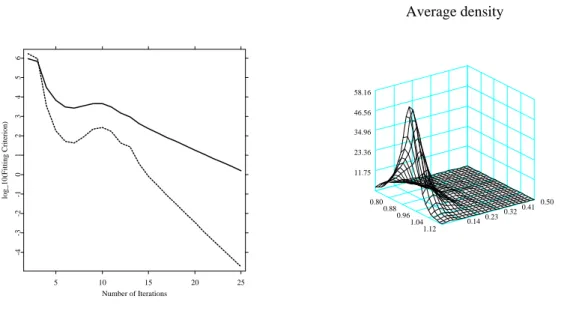
Figure 3: Left panel: convergence in the IVS models. Solid line shows the L1, the dotted line the L2 measure of convergence. Total number of iterations is 25. Right panel: average density p(u) =ˆ I−1PI
i=1pˆi(u). Bandwidths are h1 = 0.03 for moneyness and h2 = 0.04 for time to maturity.
the basis functions change relative to the optimal bandwidth h∗. We compute:
Vβb(hk) = v u u t
L
X
l=0
Var{|βbi,l(hk)−βbi,l(h∗)|}, (20)
and Vmb(hk) = v u u t
L
X
l=0
Var{|mbl(u;hk)−mbl(u;h∗)|}, (21) where hk runs over the values given in Table 3.2, and Var(x) denotes the variance of x. It is seen that changes in mb are 10 to 100 times higher in magnitude than those for β. Thisb corroborates the approximation in (32) that treats the factor loadings as known. In Figure3 we display an L1- and an L2-convergence measure of the algorithm, see Appendix A for definitions. Convergence is achieved quickly, and we stop the iterations after 25 cycles, when the L2 was less than 10−5.
Figures 4to 6display the functions mb1 to mb4 together with their contour plots. We do not
h1 h2 ΞAIC1 ΞAIC2 V
βb V
mb
0.01 0.02 0.000737 0.00151 0.015 0.938 0.01 0.04 0.000741 0.00150 0.003 0.579 0.01 0.06 0.000739 0.00152 0.005 0.416 0.01 0.08 0.000736 0.00163 0.011 0.434 0.02 0.02 0.001895 0.00237 0.104 3.098 0.02 0.04 0.000738 0.00150 0.001 0.181 0.02 0.06 0.000741 0.00151 0.004 0.196 0.02 0.08 0.000742 0.00156 0.008 0.279 0.02 0.10 0.000744 0.00162 0.011 0.339 0.03 0.02 0.002139 0.00256 0.111 3.050 0.03 0.04 0.000739 0.00149 − −
0.03 0.06 0.000743 0.00152 0.004 0.180 0.03 0.08 0.000743 0.00156 0.008 0.273 0.03 0.10 0.000744 0.00162 0.011 0.337 0.04 0.02 0.002955 0.00323 0.138 3.017 0.04 0.04 0.000743 0.00151 0.001 0.088 0.04 0.06 0.000746 0.00154 0.005 0.211 0.04 0.08 0.000745 0.00157 0.008 0.293 0.04 0.10 0.000746 0.00163 0.012 0.353 0.05 0.02 0.003117 0.00341 0.142 2.962 0.05 0.04 0.000748 0.00155 0.001 0.148 0.05 0.06 0.000749 0.00157 0.005 0.241 0.05 0.08 0.000748 0.00160 0.008 0.312 0.05 0.10 0.000749 0.00167 0.012 0.368 0.06 0.02 0.003054 0.00343 0.139 2.923 0.06 0.04 0.000755 0.00160 0.002 0.193 0.06 0.06 0.000756 0.00163 0.005 0.268 0.06 0.08 0.000754 0.00166 0.009 0.330 0.06 0.10 0.000754 0.00172 0.012 0.383
Table 2: Bandwidth selection via AIC as given in (33) and (34) for different choices of h:
h1 refers to moneyness andh2 to time to maturity measured in years; the bandwidth chosen is highlighted in bold. In all cases L = 3. Vβb and V
mb measure the change in βb and mb as functions of h relative the optimal bandwidth h∗ = (0.03,0.04)>, compare (20) and (21).
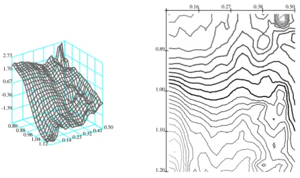
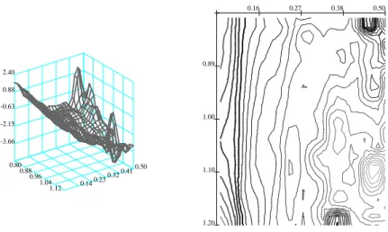
display the invariant function mb0, since it essentially is the zero function of the affine space fitted by the data: both mean and median are zero up to 10−2 in magnitude. We believe this to be estimation error. The remaining functions exhibit more interesting patterns: mb1 in Figure 4 is positive throughout, and mildly concave. There is little variability across the term structure. Since this function belongs to the weights with highest variance, we interpret it as the time dependent mean of the (log)-IVS, i.e. a shift effect. Function mb2, depicted in Figure 5, changes sign around the at-the-money region, which implies that the smile deformation of the IVS is exacerbated or mitigated by this eigenfunction. Hence we consider this function as a moneyness slope effect of the IVS. Finally,mb3 is positive for the very short term contracts, and negative for contracts with maturity longer than 0.1 years, Figure 6. Thus, a positive weight in βb3 lowers short term implied volatilities and increases long term implied volatilities: mb3 generates the term structure dynamics of the IVS, it provides a term structure slope effect. These observations are line with the results of earlier studies on the IVS, Skiadopoulos et al. (1999),Cont and da Fonseca (2002), and Fengler et al.(2003). It is important to remark that the eigenfunctions appear quite rough, which is due the small bandwidths we use here for demonstration. Depending on the specific application, for instance the one we consider in Section 4it may be advisable to employ somewhat larger bandwidths.
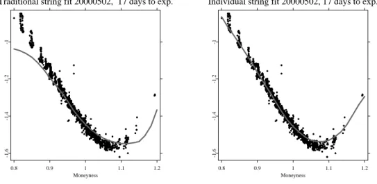
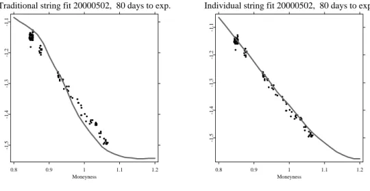
To appreciate the power of the DSFM, we inspect again the case of 20000502. In Figure 7, we compare a Nadaraya-Watson estimator (left panel) with the DSFM (right panel). In the first case, the bandwidths are increased to h= (0.06,0.25)> in order to remove all holes and excessive variation in the fit, while for the latter the bandwidths are kept ath= (0.03,0.04)>. While both fits look similar at first sight, the differences are best visible when both cases are contrasted for each time to maturity string separately, Figures 8 to 11. Generally, the standard Nadaraya-Watson fit exhibits a strong directional bias, especially in the wings. The DSFM is not entirely unbiased either, but clearly the fit is superior.
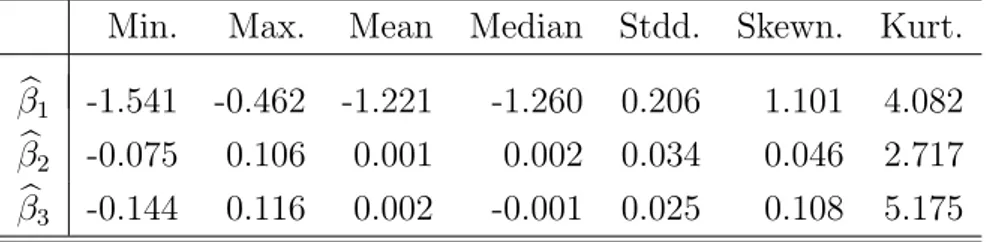
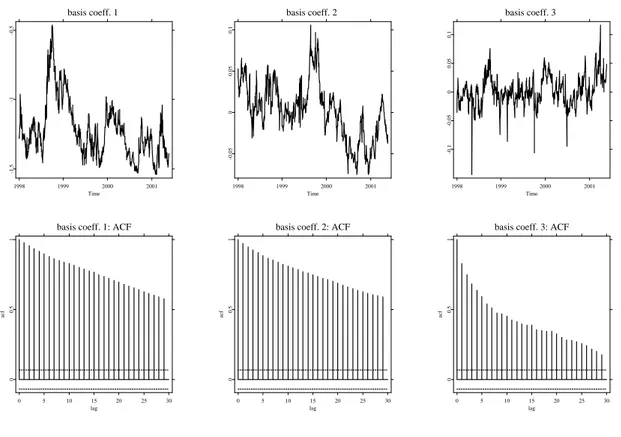
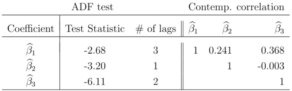
Figure 12 shows the time series of βb1 to βb3 and their correlograms. Summary statistics are given in Table 3 and contemporaneous correlation in the right part of Table 4. The ADF tests at the 5% level, left part of Table 4, indicate a unit root for βb1 and βb2. Thus, one may model first differences of the first two loading series together with the levels of βb3 in a parsimonious VAR framework. Alternatively, since the results are only marginally
0.14 0.23 0.32 0.41 0.50 0.80
0.88 0.96
1.04 1.12 0.70
0.84 0.99 1.14 1.28
0.89
1.00
1.10
1.20
0.16 0.27 0.38 0.50
Figure 4: Factor mb1 in the left panel (moneyness lower left axis, lower right axis time to maturity). Right panel shows contour plots of this function (moneyness left axis, time to maturity top). Lines are thick for positive level values, thin for negative ones. The gray scale becomes increasingly lighter the higher the level in absolute value. Stepwidth between contour lines is 0.028, estimated from ODAX data 199801-200105.
Min. Max. Mean Median Stdd. Skewn. Kurt.
βb1 -1.541 -0.462 -1.221 -1.260 0.206 1.101 4.082 βb2 -0.075 0.106 0.001 0.002 0.034 0.046 2.717 βb3 -0.144 0.116 0.002 -0.001 0.025 0.108 5.175
Table 3: Summary statistics on (βb1,βb2,βb3)> from Section3.2.
significant, one may estimate the levels of the loading series in a rich VAR model. We opt for the latter choice and use a VAR(2) model, Table 5. The estimation also includes a constant and two dummy variables, assuming the value one right at those days and one day after, when the corresponding IV observations of the minimum time to maturity string (10 days to expiry) were to be excluded from the estimation of the DSFM. This is to capture possible seasonality effects introduced from the data filter.
The estimation results are displayed in Table 5. In the equations of βb1 and βb2 the constants
0.14 0.23 0.32 0.41 0.50 0.80
0.88 0.96
1.04 1.12 -1.39
-0.36 0.67 1.70 2.73
0.89
1.00
1.10
1.20
0.16 0.27 0.38 0.50
Figure 5: Factor mb2 in the left panel (moneyness lower left axis, lower right axis time to maturity). Right panel shows contour plots of this function (moneyness left axis, time to maturity top). Lines are thick for positive level values, thin for negative ones. The gray scale becomes increasingly lighter the higher the level in absolute value. Stepwidth between contour lines is 0.225, estimated from ODAX data 199801-200105.
and dummies are weakly significant, but not shown for the sake of clarity. As is seen all factor loadings follow AR(2) processes. There are also a number of remarkable cross dynamics. Exploiting these cross dynamics is vital for the model’s performance, as shall be seen in the subsequent prediction contest.
3.3 Prediction contest
We now study the prediction performance of our model compared with a benchmark model.
Model comparisons that have been conducted, for instance by Bakshi et al. (1997),Dumas et al. (1998), and Bates (2000), often reveal that simple trader models perform better than more sophisticated models. These models used by professionals simply assert that today’s implied volatility is tomorrow’s implied volatility. There are two versions: the sticky strike assumption pretends that implied volatility is constant at fixed strikes. The sticky moneyness version claims the same for implied volatilities observed at a fixed moneyness,Derman(1999).
0.14 0.23 0.32 0.41 0.50 0.80
0.88 0.96
1.04 1.12 -3.66
-2.15 -0.63 0.88 2.40
0.89
1.00
1.10
1.20
0.16 0.27 0.38 0.50
Figure 6: Factor mb3 in the left panel (moneyness lower left axis, lower right axis time to maturity). Right panel shows contour plots of this function (moneyness left axis, time to maturity top). Lines are thick for positive level values, thin for negative ones. The gray scale becomes increasingly lighter the higher the level in absolute value. Stepwidth between contour lines is 0.240, estimated from ODAX data 199801-200105.
Model fit 20000502
0.14 0.23 0.32 0.41 0.50 0.80
0.88 0.96
1.04 1.12 -1.47
-1.31 -1.16 -1.00 -0.85
Semiparametric factor model fit 20000502
0.14 0.23 0.32 0.41 0.50 0.80
0.88 0.96
1.04 1.12 -1.47
-1.31 -1.16 -1.00 -0.85
Figure 7: Nadaraya-Watson estimator with h = (0.06,0.25)> and DSFM with h = (0.03,0.04)> for 20000502.
Traditional string fit 20000502, 17 days to exp.
0.8 0.9 1 1.1 1.2
Moneyness
-1.6-1.4-1.2-1
Individual string fit 20000502, 17 days to exp.
0.8 0.9 1 1.1 1.2
Moneyness
-1.6-1.4-1.2-1
Figure 8: Bias comparison of the Nadaraya-Watson estimator with h = (0.06,0.25)> (left panel) and the semi-parametric factor model with h = (0.03,0.04)> (right panel) for the 17 days to expiry data (black bullets) on 20000502.
Traditional string fit 20000502, 45 days to exp.
0.8 0.9 1 1.1 1.2
Moneyness
-1.5-1.4-1.3-1.2-1.1
Individual string fit 20000502, 45 days to exp.
0.8 0.9 1 1.1 1.2
Moneyness
-1.5-1.4-1.3-1.2-1.1
Figure 9: Bias comparison of the Nadaraya-Watson estimator with h = (0.06,0.25)> (left panel) and the semi-parametric factor model with h = (0.03,0.04)> (right panel) for the 45 days to expiry data (black bullets) on 20000502.
Traditional string fit 20000502, 80 days to exp.
0.8 0.9 1 1.1 1.2
Moneyness
-1.5-1.4-1.3-1.2-1.1
Individual string fit 20000502, 80 days to exp.
0.8 0.9 1 1.1 1.2
Moneyness
-1.5-1.4-1.3-1.2-1.1
Figure 10: Bias comparison of the Nadaraya-Watson estimator with h = (0.06,0.25)> (left panel) and the semi-parametric factor model with h = (0.03,0.04)> (right panel) for the 80 days to expiry data (black bullets) on 20000502.
Traditional string fit 20000502, 136 days to exp.
0.8 0.9 1 1.1 1.2
Moneyness
-1.6-1.5-1.4-1.3-1.2-1.1
Individual string fit 20000502, 136 days to exp.
0.8 0.9 1 1.1 1.2
Moneyness
-1.6-1.5-1.4-1.3-1.2-1.1
Figure 11: Bias comparison of the Nadaraya-Watson estimator with h = (0.06,0.25)> (left panel) and the semi-parametric factor model with h= (0.03,0.04)> (right panel) for the 136 days to expiry data (black bullets) on 20000502.
basis coeff. 1
1998 1999 2000 2001
Time
-1.5-1-0.5
basis coeff. 2
1998 1999 2000 2001
Time
-0.0500.050.1
basis coeff. 3
1998 1999 2000 2001
Time
-0.1-0.0500.050.1
basis coeff. 1: ACF
0 5 10 15 20 25 30
lag
00.51
acf
basis coeff. 2: ACF
0 5 10 15 20 25 30
lag
00.51
acf
basis coeff. 3: ACF
0 5 10 15 20 25 30
lag
00.51
acf
Figure 12: Upper panel: time series of weights (βb1,βb2,βb3)>. Lower panel: autocorrelation functions.
We use the sticky moneyness model as our benchmark. There are two reasons for this choice:
first, from a methodological point of view, as has been shown byBalland(2002) and Daglish et al. (2003), the sticky strike rule as an assumption on the stochastic process governing implied volatilities, is not consistent with the existence of a smile. The sticky moneyness rule, however, can be. Second, since we estimate our model in terms of moneyness, sticky moneyness rule is most natural.
Our methodology in comparing prediction performance is as follows: as presented in Sec- tion 3.2, the resulting times series of latent factors βbi,l is replaced by a times series model with fitted values βei,l(ˆθ) based on βbi0,l with i0 ≤ i−1 ,1 ≤ l ≤ L, where ˆθ is a vector of estimated coefficients seen in Table5. As in Section2, we employ a variant of ΞAIC1 based on thefittedvalues as an asymptotically unbiased estimate of mean square prediction error. The criterion is penalized with the dimension of the model, dim(θ) = 27 (six VAR-coefficients in
ADF test Contemp. correlation Coefficient Test Statistic # of lags βb1 βb2 βb3
βb1 -2.68 3 1 0.241 0.368
βb2 -3.20 1 1 -0.003
βb3 -6.11 2 1
Table 4: Left part: ADF tests on βb1 to βb3 for the full IVS model, intercept included in each case. Third column gives the number of lags included in the ADF regression. For the choice of lag length, we started with four lags, and subsequently deleted lag terms, until the last lag term became significant at least at a 5% level. MacKinnon critical values for rejecting the hypothesis of a unit root are -2.87 at 5% significance level, and -3.44 at 1% significance level.
Right part: contemporaneous correlation matrix.
three equations plus a constant and two dummy variables), see Appendix A.
This criterion, denoted by ΞeAIC, is compared with the squared one-day prediction error of the sticky moneyness (StM) model:
ΞStM def= N−1
I
X
i Ji
X
j
(Yi,j−Yi−1,j0)2 . (22)
In practice, since one hardly observes Yi,j at the same moneyness as in i −1, Yi−1,j0 is obtained via a localized interpolation of the previous day’s smile. Time to maturity effects are neglected, and observations, the previous values of which are lost due to expiry, are deleted from the sample. Running the model comparison shows:
ΞStM = 0.00476 versus ΞeAIC = 0.00439 .
Thus, the model comparison reveals that the DSFM is approximate 10% better than the sticky moneyness model. This is a substantial improvement given the high variance in implied volatility and financial data in general.
Equation
Dependent variable βb1,i βb2,i βb3,i
βb1,i−1 0.978 -0.009 0.047
[24.40] [-1.21] [ 3.70]
βb1,i−2 0.004 0.012 -0.047
[ 0.08] [ 1.63] [-3.68]
βb2,i−1 0.182 0.861 0.134
[ 0.92] [ 23.88] [ 2.13]
βb2,i−2 -0.129 0.109 -0.126
[-0.65] [ 3.03] [-2.01]
βb3,i−1 0.115 -0.019 0.614
[ 0.97] [-0.89] [ 16.16]
βb3,i−2 -0.231 0.030 0.248
[-1.96] [ 1.40] [ 6.60]
R¯2 0.957 0.948 0.705
F-statistic 2405.273 1945.451 258.165
Table 5: Estimation results of an VAR(2) of the factor loadings βbi. t-statistics given in brackets, R¯2 denotes the adjusted coefficient of determination. The estimation includes an intercept and two dummy variables (both not shown), which assume the value one right at those days and one day after, when the corresponding IV observations of the minimum time to maturity string (10 days to expiry) were to be excluded from the estimation of the DSFM.
4 Hedging in local volatility models using the DSFM
Local volatility models are one-factor models, i.e. it is assumed that the asset price dynamics are governed by the stochastic differential equation
dSt
St =µ dt+σ(St, t)dWt, (23) where Wt is a Brownian motion, µ denotes the drift, and σ(St, t) the local volatility func- tion which depends on the asset price and time, only. In local volatility pricers, the IVS is
employed to calibrate the local volatility function to the market. Then, the BS partial dif- ferential equation with generalized volatility function is solved for pricing the exotic options, Andersen and Brotherton-Ratcliffe (1997) and Dempster and Richards (2000). Therefore, unlike to the BS model, prices depend on the entire IVS, and not simply on the implied volatility at a specific strike. In consequence, the notion of vega hedging needs to be gener- alized. A usual attempt to respond to this problem, is to define a so called ‘parallel-shift-vega’
which corresponds to the sensitivity of the option price with respect to a parallel shift of the whole IVS. It is calculated via bumping the IVS by a certain factor and computing the difference quotient. From our empirical analysis, however, it is obvious that the IVS displays much more sophisticated dynamics as is manifest in the moneyness slope and term structure slope effects. While an up-and-down shift of the IVS may be the most important factor, the parallel-shift-vega leaves the slope and term structure risks, which the exotic option is exposed to, unhedged. Depending on the specific payoff profile of the option, these risks, however, can be of substantial size. For instance, for down-and-out puts, the probability of hitting the barrier is very much determined by the slope of the smile. In this case, it is desirable to hedge the slope risks of the IVS.
The DSFM gives a decomposition of the IVS into its most important factors. For path- dependent options, we therefore propose to define the hedge in terms of these factors. More precisely, given the decomposition
ˆ
σt(κ, τ) = exp
L
X
l=0
βbt,lmbl
!
, (24)
the β1-greek, ∂β∂
1, defines the sensitivity of the option with respect to up-and-down shifts of the (log)-IVS. Theβ2-greek, ∂β∂
2, is a slope-shift-vega of the (log)-IVS, and so on. For setting up a hedge, one needs to define portfolios HP1, HP2, . . . consisting of plain vanilla options that have approximately the same first order expansion in terms of these beta-greeks. Given the hedge-ratios the residual delta risk is hedged with the underlying. The particular nature of the hedge portfolio depends on the exotic option to be hedged, but may also depend on general targets in risk management such as to reduce gamma risks.
To make our approach more precise, we concentrate on the two-factor case with two hedge portfoliosHP1 andHP2 and the aforementioned down-and-out putPdo. First, one computes the sensitivities of the hedge portfolios and the barrier option with respect to β1 andβ2, for