SFB 649 Discussion Paper 2009-019
A Joint Analysis of the KOSPI 200 Option and ODAX Option Markets
Dynamics
Ji Cao*
Wolfgang Härdle*
Julius Mungo*
*Humboldt-Universität zu Berlin, Germany
This research was supported by the Deutsche
Forschungsgemeinschaft through the SFB 649 "Economic Risk".
http://sfb649.wiwi.hu-berlin.de ISSN 1860-5664
SFB 649, Humboldt-Universität zu Berlin
S FB
6 4 9
E C O N O M I C
R I S K
B E R L I N
A Joint Analysis of the KOSPI 200 Option and ODAX Option Markets Dynamics
∗Ji Cao†, Wolfgang K. H¨ardle ‡, Julius Mungo §
Abstract
As a function of strike and time to maturity the implied volatility estimation is a challenging task in financial econometrics. Dynamic Semiparametric Factor Models (DSFM) are a model class that allows for the estimation of the implied volatility surface (IVS) in a dynamic context, employing semiparametric factor functions and time-varying loadings. Because financial asset volatilities move over time, across assets and over markets, this paper analyses volatility interaction be- tween German and Korean stock markets. As proxy for the volatility, factor loadings series derived from a DSFM application on option prices are employed. We examine volatility transmission between the markets under the vector autoregressive (VAR) model framework. Our results show that a shock in the volatility of one market may not translate directly into greater uncertainty in another market and it is unlikely that portfolio investors can benefit from diversification among these markets due to cointegration.
Keywords: implied volatility surface, dynamic semiparametric fac- tor model, VAR, cointegration
JEL classification: C14; G12
∗The financial support from the Deutsche Forschungsgemeinschaft via SFB 649
“ ¨Okonomisches Risiko”, Humboldt-Universit¨at zu Berlin is gratefully acknowledged.
†Corresponding author. Institute for Statistics and Econometrics of Humboldt- Universit¨at zu Berlin, Spandauer Straße 1, 10178 Berlin, Germany. Email: ji.cao@wiwi.hu- berlin.de.
‡Center for Applied Statistics and Economics, Humboldt-Universit¨at zu Berlin, Span- dauer Straße 1, 10178 Berlin, Germany.
§Institute for Statistics and Econometrics of Humboldt-Universit¨at zu Berlin, Span- dauer Straße 1, 10178 Berlin, Germany.
1 Introduction
As one of the most important parameters in financial markets, volatility has attracted a lot of attention. In derivatives pricing and hedging, volatility is a key issue and because volatility is unknown, one studies the implied volatility (IV) which is derived from the Black-Scholes formula (BS). By plugging the observed option price into the BS formula it is straightforward to calculate the implied volatility. Implied volatility is seen as a mapping from time t, moneyness κ (a measure of strike) and time to maturity τ, bσ: (t, κ, τ)→σbt(κ, τ).
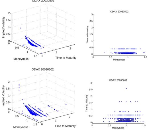
Calculating implied volatilities at different strikes and maturities yields an implied volatility surface (IVS). One challenge in IVS modelling is that the data have a degenerated design: due to market conventions, maturities only have a small number of values such as one, two, three, six, nine and twelve months to expiry on the date of issue. This fact leads to a string structure of observations in IVS. As time passes these strings change their shape and location randomly. Figure 1 displays implied volatility of the ODAX on 2 May and 2 June, 2003. The implied volatilities on these two days show different patterns. On 2 May, the largest implied volatility is about 1, and it is about 2 on 2 June. There are three different expiration times on 2 May but eight on 2 June.
Dynamic semiparametric factor models are designed to capture these fea- tures of the IVS with low-dimensional factor functions and time-varying factor loadings. The IVS is approximated by unknown factor functions moving in a finite dimensional function space. The finite dimensional fits are obtained in the local neighbourhood of strikes and maturities, for which implied volatilities are recorded on the specific day. Surface estimation and dimension reduction is achieved in one single step. This approach can be seen as a combination of functional principal component analysis, nonpara- metric curve estimation and backfitting for additive models. The DSFM is generally expressed as
Yt,j =m0(Xt,j) +
L
X
l=1
Zt,lml(Xt,j) +εt,j, (1)
whereYt,j is the log-implied volatility for optionj on dayt,tis an index of day (t= 1, . . . , T) andj is an index of options on dayt(j= 1, . . . , J). Xt,j
is two-dimensional covariables,Xt,j = (κt,j, τt,j) withκt,j the moneyness (we define moneynessκt,j def= KFt,j
t,j, whereKt,j is the strike andFt,j is the future price.) and τt,j time to maturity. ml is time-invariant factor function and
0 0.5
1
1.5 0 1
2 0
0.5 1 1.5 2
Time to Maturity ODAX 20030502
Moneyness
Implied Volatility
0 0.5 1 1.5
0 0.5 1 1.5 2 2.5 3
ODAX 20030502
Moneyness
Time to Maturity
0 0.5
1
1.5 0 1
2 0
0.5 1 1.5 2
Time to Maturity ODAX 20030602
Moneyness
Implied Volatility
0 0.5 1 1.5
0 0.5 1 1.5 2 2.5 3
ODAX 20030602
Moneyness
Time to Maturity
Figure 1: Upper left: implied volatility of ODAX on 2 May, 2003. (money- ness lower left axis, time to maturity lower right axis). Upper right: Data design of ODAX on 2 May, 2003. Lower left: implied volatility of ODAX on 2 June, 2003. Lower right: Data design of ODAX on 2 June, 2003.
Zt,l is loading for factor ml. εt,j is an unknown error term with E(εt,j) = 0 and E(ε2t,j) < ∞. After estimating unknown factor function ml and corre- sponding loading Zt,l, implied volatility can be calculated given a desired point (κt,j, τt,j).
In a study related to the DSFM estimation, Park et al. (2009) have shown that the covariance structure of the estimated loading series converges in probability to the covariance structure of the unobservable loading series.
This indicates that the additional error incurred by using Zbt instead of Zt
is negligible for largeT. This asymptotic equivalence of the autocovariance structures carries over to classical estimation and testing procedures within the VAR model framework.
This paper applies the DSFM to estimate IVS of the Korean Stock Index (KOSPI 200) options and the ODAX. The estimation result is discussed and a joint analysis between two markets is studied. The paper is organised as follows: Section 2 describes data preparation and implied volatility calcu- lation. The DSFM model fit is discussed in Section 3. Section 4 presents a joint analysis of the KOSPI option and the ODAX factor loading series dynamics. Conclusion is presented in section 5.
2 Data and Implied volatility calculation
The data set contains tick statistics on KOSPI 200 option from the Korea Exchange and the ODAX from Eurex over the period from January 2003 to December 2003. The KOSPI 200 (Korea Composite Stock Price Index) is the index of 200 major companies’ stocks traded on the Stock Market Division of the Korea Exchange. It is one of the most actively traded indices in the world. The Korea Exchange (KRX) is by transactional volume the largest derivatives exchange in the world. Deutscher Aktien IndeX 30 (German stock index) is a Blue Chip stock market index consisting of the 30 major German companies traded on the Frankfurt Stock Exchange. Its option ODAX is traded on Eurex (Germany and Switzerland) which is by far the world’s largest international market organiser for the trading and settlement of futures and options on shares and share indices, as well as of interest rate derivatives. Both KOSPI 200 option data and ODAX data are recorded per transaction, that is, each observation contains information on option price, strike price, settlement time, maturity, etc.
One of the problems we face when calculating the implied volatility is the intraday underlying price. In Fengler et al. (2007) the intraday underlying price is used for IVS estimation. However, neither KOSPI data nor ODAX
data in our case contains underlying price. In Fengler et al. (2007) the intra- day future price within one-minute intervals is used to derive the underlying price. While for ODAX data corresponding future prices can be found in our case, we have not obtained any information of intraday futures price for KOSPI 200.
Another approach to obtain the intraday underlying price is to use put-call parity:
Ct=Pt+St−Dt−Ke−rτ, (2) where Ct and Pt are prices of European call and put options on the same underlying with the same strike price K and same maturity T. Dt is the discounted value of dividend paid by underlying during the time to maturity τ =T−t. r and St are the interest rate and underlying price, respectively.
Based on corresponding put and call option prices, the underlying priceSt can be derived.
Unfortunately, there are only a few cases where pair of corresponding call and put contracts can be found in our data. Thus, intraday implied volatility cannot be calculated under these circumstances.
While it is difficult to find intraday underlying prices for both markets, acquiring closing prices is relatively easy, therefore, instead of using intraday prices, we use the closing prices in our analysis. Together with the last traded contract for each series of options - options with the same type, same maturity, same strike and traded on the same day, aclosing implied volatility is calculated. Last traded contracts are extracted from the whole data set according to their settlement time. Many of these last traded contracts are settled between 14:00 and 15:15 hrs on the Korea Exchange and between 17:00 and 19:00 hrs on the Eurex - both near to the close time of their underlying markets. (On a normal trading day, trading of the KOSPI 200 option at the Korean Exchange ends at 15:15 hrs. On regular trading days, ODAX trading ends at 17:30 hrs with a post trading phase ending at 21:00 hrs.) At the same time, it is, however, also possible that the last traded contract is settled as early as 9:15 hrs - shortly after the market opens, thus an implied volatility based on this contract may not reflect the state of the market at close. Strictly speaking, using last traded contracts, together with closing underlying prices does not necessarily lead to closing implied volatility. To improve accuracy, some adjustments or smoothing techniques should be used in further study.
To calculate implied volatility, the interest rate for the KOSPI 200 option is the daily Korean treasury bill rate, for ODAX it is the daily EURIBOR rate in the same period.
After extracting the last traded contracts from the whole data set, our sam- ple size reduces and we are left with only about 40 observations per day. A linear interpolation is used in order to represent the data on a regular grid.
Options on the same day and with the same maturity are grouped together and interpolated with respect to the moneyness gridκ∈[0.8,1.2] with 1000 points. Furthermore, call option and put option are interpolated separately.
A new problem arises here: for both the KOSPI 200 option and the ODAX markets, implied volatilities calculated from put options and call options are different, even if they have the same strike, same maturity and same spot.
In Fengler et al. (2007) a correction algorithm is used to obtain an adjusted underlying price, based on which, the put and call implied volatilities are the same. This algorithm (3) is based on the future price formula and put-call parity.
S˜t=e−rF(TF−t)Ft+ ∆Dt,TH,TF, (3) where ˜St is the adjusted underlying price, rF is the interest rate used in deriving the underlying price from the future price,TF is the future’s matu- rity time,Ftis the future price,TH isthe option’s maturity time, ∆Dt,TH,TF
is the dividend difference calculated from put-call parity (2) and the future price formula Ft =erF(TF−t)St−∆Dt,TF, ∆Dt,TF is the dividend used for calculating future price.
However, it is a different situation in our case. Firstly, our underlying price is not obtained from the future price, but directly from the closing price in the underlying markets. Secondly, as stated before, there are only a few corresponding put and call options in our case, thus put-call parity cannot be used. Consequently, we don’t apply algorithm (3) in our case. Instead, after interpolating put and call implied volatilities separately, we take the average of these two implied volatility series. Our algorithm of interpolation and average taking is described in detail as follows:
1. For each day, options (implied volatilities) with the same maturity are grouped together asIVt,jC(κm) andIVt,jP(κn). t is day index. j is group index on this day - index for different maturity. C is call and P is put. κm and κn are moneyness for calls and puts respectively, m= 1, . . . , M,n= 1, . . . , N.
2. For each group of these optionsIVt,jC(κm) andIVt,jP(κn), (a) if both the number of calls
M
P
m=1
m ≥ 3 and the number of puts
N
P
n=1
n ≥ 3, call implied volatility and put implied volatility are
linearly interpolated separately with respect to moneyness κ on gridκ∈[0.8,1.2] with 1000 points.
IVt,jC(κl) = κl−κm
κm+1−κmIVt,jC(κm+1) + κm+1−κl
κm+1−κmIVt,jC(κm), (4) and
IVt,jP(κl) = κl−κn
κn+1−κnIVt,jP(κn+1) + κn+1−κl
κn+1−κnIVt,jP(κm), (5) whereκl is desired moneyness point, l∈[1,1000], κl ∈[0.8,1.2].
κm and κm+1 are two closest observations to κl, withκm< κl<
κm+1. If max(κm) < κl or κl <min(κm), a constant extrapola- tion is used. Forκn and κn+1 is the same.
Then, an average of IVt,jC(κl) and IVt,jP(κl) is taken as the final implied volatility,
IVt,j(κl) = IVt,jC(κl) +IVt,jP(κl)
2 (6)
(b) if only the number of calls PM m=1
m≥3, while the number of puts PN
n=1
n <3, call implied volatilities are interpolated with (4). Put implied volatilities are dropped. Final implied volatilities are these interpolated call implied volatilities,
IVt,j(κl) =IVt,jC(κl) (7) (c) similarly, if only the number of puts
N
P
n=1
n≥3, but the number of calls
M
P
m=1
m <3, put implied volatilities are interpolated with (5).
Call implied volatilities are dropped. Final implied volatilities are these interpolated put implied volatilities,
IVt,j(κl) =IVt,jP(κl) (8) (d) if both the number of calls
M
P
m=1
m < 3 and the number of puts
N
P
n=1
n <3, final implied volatilities are the original observations, IVt,j(κm) =IVt,jC(κm)
IVt,j(κn) =IVt,jP(κn). (9)
0.8 0.9 1 1.1 1.2 0.15
0.2 0.25 0.3
KOSPI 200 20030901
Moneyness
Implied Volatility
0.8 0.9 1 1.1 1.2
0.15 0.2 0.25 0.3
KOSPI 200 20030901
Moneyness
Implied Volatility
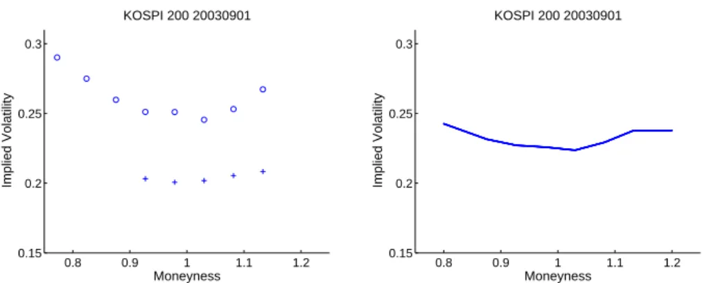
Figure 2: Implied volatility of last traded KOSPI 200 options with 102 days to maturity on 1 September, 2003. Left panel: original data, before interpo- lation. Call options are ”+”, put options are ”o”. Right panel: with linear interpolation and averaging.
Figure 2 is an example of one group of KOSPI 200 option data on 1 Septem- ber, 2003. These contracts have 102 days to maturity. The left panel shows the original data - the last traded contracts taken from the entire data set.
The right panel is based on the left panel, with interpolating call and put options separately and then averaging.
3 Model fit
The estimates mbl (l = 0, . . . , L) and Zbt,l (t = 1, . . . , T; l = 1, . . . , L) are defined as minimisers of the following least squares criterion (Zbt,0def
= 1):
T
X
t=1 Ji
X
j=1
Z ( Yt,j−
L
X
l=0
Zbt,lmbl(u) )2
Kh(u−Xt,j)du. (10) Here, Kh denotes a two-dimensional product kernel, Kh(u) = kh1(u1)× kh2(u2),h= (h1, h2), based on the one-dimensional kernelkh(v)def= h−1k(h−1v).
In (10) the minimisation runs over all the functions mbl: R2 → R and all valuesZbt,l ∈R. In order to derive an estimator of the DSFM we proceed in the following way. (For the technical details we refer to Borak et al. (2005), Fengler et al. (2007) and Park et al. (2009).) For an l0 with 1≤l0 ≤L,for δ >0 and a functiong, we replace in (10)mbl0 by mbl0+δgand take the first
derivative with respect toδ at the point δ=0. This yields
T
X
t=1 Jt
X
j=1
Z ( Yt,j−
L
X
l=0
Zbt,lmbl(u) )
Zbt,l0Kh(u−Xt,j)du= 0. (11) Since the equation holds for all functions g, it implies that for 1 ≤ l0 ≤ L and for allu
T
X
t=1 Jt
X
j=1
( Yt,j−
L
X
l=0
Zbt,lmbl(u) )
Zbt,l0Kh(u−Xt,j) = 0. (12) By replacingZbt,l0byZbt,l0+δin (10) and again taking derivatives with respect toδ, we get for 1≤l0 ≤L and 1≤t0≤T:
Jt0
X
j=1
Z ( Yt0,j−
L
X
l=0
Zbt0,lmbl(u) )
mbl0(u)Kh(u−Xt0,j)du= 0. (13) Using the following notation, for 1≤t≤T
pbt(u) = 1 Jt
Jt
X
j=1
Kh(u−Xt,j), (14)
qbt(u) = 1 Jt
Jt
X
j=1
Kh(u−Xt,j)Yt,j, (15)
from (12) - (13) we get, for 1≤l0≤Land 1≤t≤T:
T
X
t=1
JtZbt,l0bqt(u) =
T
X
t=1
Jt
L
X
l=0
Zbt,l0Zbt,lpbt(u)mbl(u) (16)
Z
qbt(u)mbl0(u)du=
L
X
l=0
Zbt,l Z
pbt(u)mbl0(u)mbl(u)du. (17) The algorithm exploits equations (16) and (17) iteratively:
1. For an appropriate initialisation ofZbt,l(0),t= 1, . . . , T,l= 1, . . . , L get an initial estimate ofmb(0) = (mb0, . . . ,mbL)>
2. UpdateZbt,l(1),t= 1, . . . , T 3. Estimatemb(1)
4. Go to step 2,
until minor changes occur during the cycle.
The choice of the model size L is based on computing the residual sum of squares:
RV(L) = P
t
P
j
n
Yt,j−PL
l=0Zbt,lmbl(Xt,j) o2
P
t
P
j
Yt,j −Y¯ 2 , (18) where ¯Y is the overall mean of the observation. We chooseL such that the proportion of variation explained by the model among the total variation 1−RV(L) is sufficiently high.
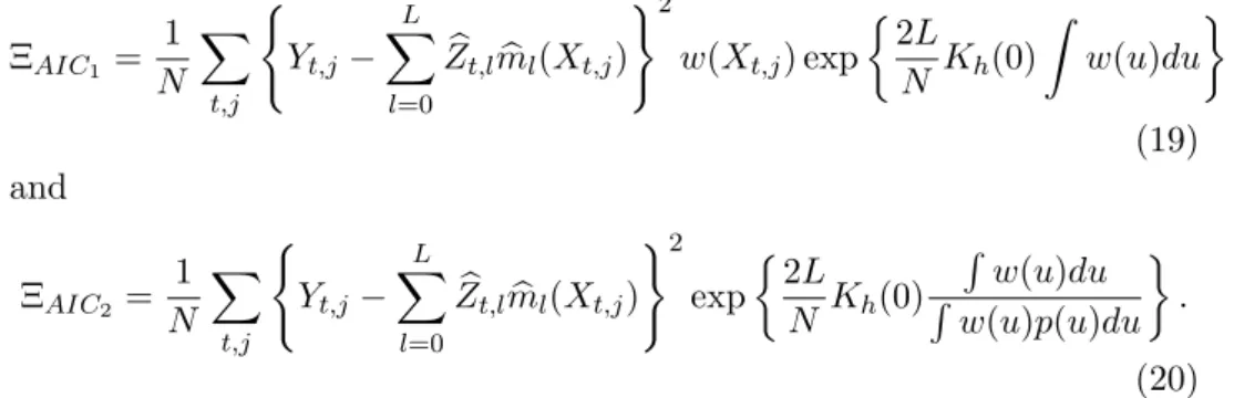
For the data-driven choice of bandwidths we take weighted AIC, as Fengler et al. (2007) did. The two criteria are:
ΞAIC1 = 1 N
X
t,j
( Yt,j−
L
X
l=0
Zbt,lmbl(Xt,j) )2
w(Xt,j) exp 2L
N Kh(0) Z
w(u)du
(19) and
ΞAIC2 = 1 N
X
t,j
( Yt,j−
L
X
l=0
Zbt,lmbl(Xt,j) )2
exp 2L
N Kh(0)
R w(u)du R w(u)p(u)du
. (20) For our implementation, we consider as outliers contracts with maturity less than 10 days, since their behaviour is irregular due to the expiry effect. We also remove observations with implied volatility smaller than 0.04 or lager than 0.8. The data set contains 829299 observations in the KOSPI 200 op- tion data (about 3371 per day) and 1113845 observations in the ODAX data (about 4546 per day). Log-implied volatilities are modeled on moneyness and time to maturity (κt,j, τt,j). The grid covers moneyness κ ∈ [0.8,1.2]
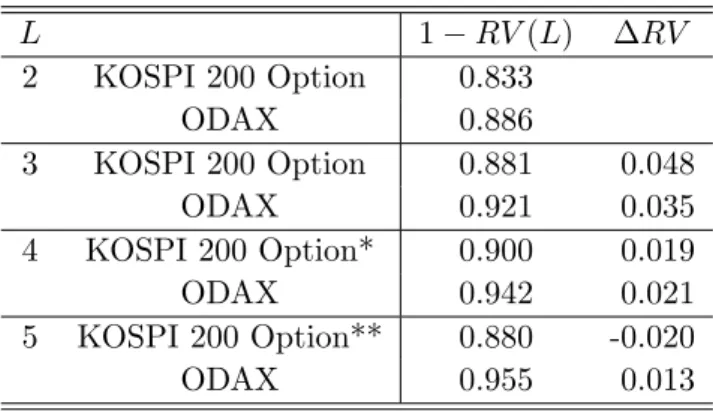
and time to maturityτ ∈[0.02,0.5] measured in years. L=3 factor functions are employed for both markets and bandwidths (0.02, 0.04) for the KOSPI 200 option and (0.02, 0.05) for the ODAX have been chosen, according to variance explained, ΞAIC1 and ΞAIC2 criterions, see Table 1. We have re- calculated the model with the same bandwidths with 2, 3, 4 and 5 dynamic factor functions, see Table 2. A choice of 3 factor functions is based on a bal- ance between model economy and efficiency - capturing as many explained variances as possible while keeping a small number of factors.
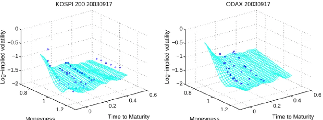
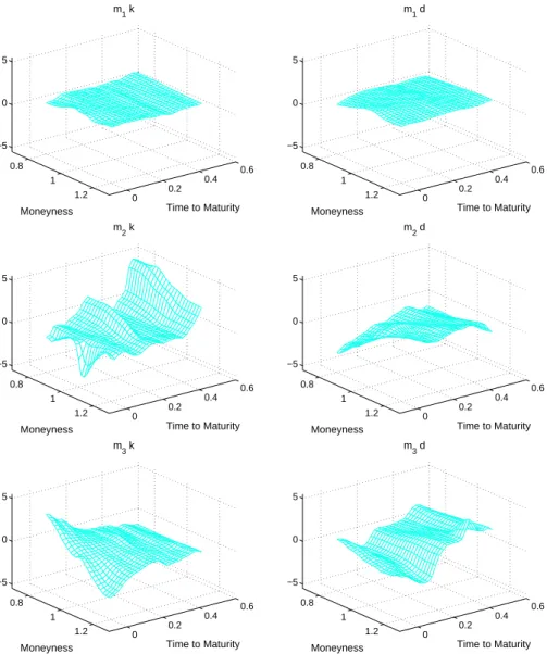
Figure 3 displays Model fits on 17 September, 2003 for both markets. The IVS of the KOSPI 200 option is flatter than the ODAX on this day. Figure 4 shows factor functionsmbi,i= 1,2,3. mb1 is positive in both markets. They
Bandwidths 1−RV(3) ΞAIC1 ΞAIC2 KOSPI 200 option (0.02, 0.04) 0.881 0.00106 0.00570
ODAX (0.02, 0.05) 0.921 0.00172 0.00612 Table 1: DSFM modelling result.
L 1−RV(L) ∆RV
2 KOSPI 200 Option 0.833
ODAX 0.886
3 KOSPI 200 Option 0.881 0.048
ODAX 0.921 0.035
4 KOSPI 200 Option* 0.900 0.019
ODAX 0.942 0.021
5 KOSPI 200 Option** 0.880 -0.020
ODAX 0.955 0.013
Table 2: Explained variance for the model size. *Bandwidth (0.02, 0.06).
**Bandwidth (0.02, 0.14).
are both relatively flat. Factormb1 can be interpreted as the time dependent mean of the (log-)IVS, ashift effect. mb2for the ODAX tends to trend upward in the moneyness axis, from negative to positive. The surface is close to 0 when moneyness is near 1. This trend is strong when time to maturity is small while it becomes weak when time to maturity increases. For mb3 of the KOSPI 200 option, a downward trend exists in maturity direction when moneyness is in the region of 0.8. The surface slopes down when time to maturity increases. This trend becomes weak when moneyness increases.
mb3 of the ODAX appears to smile in the maturity direction.
We interpret the effect of the first factor loadings such that Zb1 represents the overall level shift of the IVS. We observe in Figure 5 that Zb1 of both markets seem to have a common trend. Zb2 of the KOSPI 200 option has stronger fluctuations than that of the ODAX.
0.8 1
1.2 0
0.2 0.4
0.6
−2
−1.5
−1
−0.5 0
Time to Maturity KOSPI 200 20030917
Moneyness
Log−implied volatility
0.8 1
1.2 0
0.2 0.4
0.6
−2
−1.5
−1
−0.5 0
Time to Maturity ODAX 20030917
Moneyness
Log−implied volatility
Figure 3: DSFM fit for KOSPI 200 option (left) with bandwidths (0.02, 0.04) and the ODAX (right) with bandwidths (0.02, 0.05) on 17 September, 2003.
4 Joint dynamics of KOSPI 200 option and ODAX
Let the k dimensional vector series Zbt = (Zb1t, . . . ,Zbkt)>,t= 0, ..., T follow a VAR(p) model:
Zbt=υ+
p
X
j=1
ΦjZbt−j+εt, (21) whereυ= (υ1, . . . , υk)>is ak×1 vector of intercepts, Φjarek×kparameter matrices and the error process εt= (ε1t, . . . , εkt)> is such that
E[εt] = 0 and E(εtε>t−k) =
(0 fork6= 0 Σ fork= 0
Σ is a time invariant positive definite variance-covariance matrix of the in- novation series. In this setting we acknowledge cross dependencies between the Zbt series, i.e., each Zbt depends on its “history” and the “history” of the other series in the system. Therefore the VAR model posits a set of relationships between past lagged values of all variables in the model and the current value of each variable in the model. Descriptive statistics for the factor loadings of our model are presented in Table 3. We denote the dynamic system of factor loadings by
Zbt= (Zbt,1k ,Zbt,2k ,Zbt,3k ,Zbt,1d ,Zbt,2d ,Zbt,3d )>,
where the superscripts k and d denote loadings of KOSPI and ODAX, re- spectively. Unit root tests using the augmented Dickey-Fuller (ADF) and the Elliott et al. (ERS) testing strategies are implemented to determine
0.8 1
1.2 0
0.2
0.4 0.6
−5 0 5
Time to Maturity m1 k
Moneyness
0.8 1
1.2 0
0.2
0.4 0.6
−5 0 5
Time to Maturity m1 d
Moneyness
0.8 1
1.2 0
0.2
0.4 0.6
−5 0 5
Time to Maturity m2 k
Moneyness
0.8 1
1.2 0
0.2
0.4 0.6
−5 0 5
Time to Maturity m2 d
Moneyness
0.8 1
1.2 0 0.2
0.4 0.6
−5 0 5
Time to Maturity m3 k
Moneyness
0.8 1
1.2 0 0.2
0.4 0.6
−5 0 5
Time to Maturity m3 d
Moneyness
Figure 4: Estimated factor function mbl for KOSPI 200 option (left) and for ODAX (right) from 2 January, 2003 to 30 December, 2003.
Mean Median Min. Max. Std. Kurt. Skew.
KOSPI 200 option Zb1 -1.22 -1.28 -1.57 -0.88 0.18 1.59 0.06
Zb2 0.00 0.00 -0.5 0.62 0.09 19.16 1.29 Zb3 0.00 0.00 -0.19 0.21 0.08 2.45 -0.19 ODAX Zb1 -0.93 -0.98 -1.23 -0.56 0.18 1.94 0.49
Zb2 0.00 0.00 -0.12 0.17 0.06 2.66 0.18 Zb3 0.00 -0.01 -0.18 0.22 0.05 4.52 0.48 Table 3: Descriptive statistics for factor loadings Zb1, Zb2 and Zb3.
0 50 100 150 200
−1.5−1.0−0.50.00.5
Z1
Time (days)
0 50 100 150 200
−1.5−1.0−0.50.00.5
Z2
Time (days)
0 50 100 150 200
−1.5−1.0−0.50.00.5
Z3
Time (days)
Figure 5: Time series of factor loadings Zb1, Zb2 and Zb3 for KOSPI 200 option (blue) and ODAX (red) from 2 January, 2003 to 30 December, 2003.
KOSPI 200 option ODAX
Zb1k Zb2k Zb3k Zb1d Zb2d Zb3d ADF-AIC -1.074 -15.129** -3.409* -0.880 -16.605** -6.686**
bb 5 0 2 4 0 2
ADF-HQ -1.039 -15.129** -3.409* -0.880 -16.605** -8.656**
bb 3 0 2 4 -0 1
ERS-AIC 23.914 0.225** 2.947* 55.112 0.740** 1.313**
bb 5 0 2 4 0 2
ERS-HQ 24.783 0.225** 2.947* 55.112 0.740** 0.952**
bb 3 0 2 4 0 1
Table 4: Unit root tests for factor loadings Zb1, Zb2 and Zb3. Tests include constant. ADF-AIC and ERS-HQ refer to the ADF tests using AIC criteria and ERS tests using HQ criteria to estimate the lag length b chosen for the estimation regression of the autoregressive spectral density estimator.
Critical values for ADF test are -3.458(1%), -2.874(5%) and -2.573(10%).
Critical values for ERS test are 1.925(1%), 3.187(5%) and 4.359(10%). **
and * denote significance at the 1% and 5% level, respectively.
whether the individual series are trend stationary or difference stationary, see Table 4. We apply standard information criteria as AIC, SC and HQ to select the lag order p for our VAR. These criteria balance the trade-off between model fit and the number of parameters to be estimated and allow a fairly parsimonious model specification. We usep= 2 lags as suggested by the AIC, since we want to model the dynamic relations between the factor loading series by impulse response functions in a more flexible way.
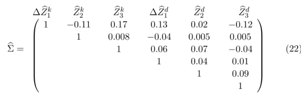
Using the lag selection criteria and the parsimony principle, a VAR(2) model Zbt = (∆Zbt,1k ,Zbt,2k ,Zbt,3k ,∆Zbt,1d ,Zbt,2d ,Zbt,3d )>, where Zbt,1k and Zbt,1d enter as first order differences, is chosen to analyse the system. The residual correlation matrix Σ, given in (22), gives us some useful information about the con-b temporaneous correlation structure, i.e. if there is overlapping information between variables. This information has implications for interpretation of
Model p Q(24) LMF(3) LBJ ARCH(1)
VAR 2 0.74 0.25 0.00 0.00
Table 5: p-values for VAR(2) diagnostic tests. Q(24) denotes an adjusted portmanteau test involving 24 autocorrelation matrices, LMF(3) is LM test for autocorrelation of order 3. LBJ represents the multivariate Lomnicki- Jaque-Bera test for nonnormality and ARCH(1) is the multivariate first- order ARCH test.
the results of the impulse responses.
Σ =b
∆Zb1k Zb2k Zb3k ∆Zb1d Zb2d Zb3d
1 −0.11 1
0.17 0.008
1
0.13
−0.04 0.06
1
0.02 0.005
0.07 0.04 1
−0.12 0.005
−0.04 0.01 0.09 1
(22)
We apply a number of standard diagnostic tests to check the adequacy of the model, see Table 5. While the estimated residuals are free from autocorrela- tion, normality and conditional homoscedasticity are rejected. Considering that the VAR is a rough approximation of the dynamics of the system, a more detailed analysis to accommodate the ARCH effects is beyond the scope of this paper.
The dynamic relations between the factors are captured by the impulse response functions. Figures 6 and 7 give the generalised impulse responses to a positive shock in the loadings series of both markets. The results indicate that there is a positive but small response between the overall changes in the risk levels of the German and Korean markets. ∆Zb1k responds only slightly positive for about 1-2 days after a shock in ∆Zb1d. On the other hand the response of ∆Zb1d to a shock in ∆Zb1k is barely positive. We take caution in interpreting the results since Zb1k and Zb1d enter the VAR model in first differences. We therefore interpret that an increase in the DAX volatility translates into a small amount of uncertainty in the Korean market. On the other hand effects of shock from the KOSPI do not translate into effective uncertainty in the DAX. Our results suggest that a shock from one market is likely to work through the other market’s system and may not induce greater impulse responses either way. This may also reflect the view of no- arbitrage relation between the two markets. We have conducted Granger
H0 Test result
∆Zb1d9∆Zb1k,Zb2k,Zb3k F(6,900) = 1.70[0.12]
∆Zb1k9∆Zb1d,Zb2k,Zb3k F(6,900) = 0.93[0.46]
∆Zb1k 9∆Zb1d,Zb2d,Zb3d F(6,900) = 1.15[0.32]
∆Zb1d9∆Zb1k,Zb2d,Zb3d F(6,900) = 2.62[0.02]
∆Zb1d9∆Zb1k F(4,446) = 4.74[0.02]
∆Zb1k9∆Zb1d F(4,446) = 0.68[0.60]
Table 6: Granger causality tests for VAR(2). 9denotes “does not Granger cause”. p-values are given in brackets. Critical values are 3.32(1%), 2.37(5%) 1.94(10%) for F(4,446) and 2.80(1%), 2.10(5%), 1.77(10%) for F(6,900).
causality tests to further investigate the relationship between these variables, see Table 6. Granger non-causality of ∆Zb1d for ∆Zb1k, Zb2d, Zb3d and of ∆Zb1d for ∆Zb1k is rejected at 5% significance level. We observe that Granger non- causality from ∆Zb1k to ∆Zb1dis not rejected. This indicates a unidirectional effect from the ODAX to the KOSPI 200 option market.
Due to the appearance of a common trend, we next investigated the cointe- gration relationship betweenZb1kandZb1d. The trace and maximum eigenvalue tests of cointegration are applied to determine whether or not the KOSPI 200 option and the ODAX first loading series share a common stochastic trend.
The test results in Table 7 show that both tests fail to reject cointegration between the factor loading seriesZb1d and Zb1k.
The existence of cointegration means that there is a long-term relationship between two variables and that they are influenced by the same stochastic trend. SinceZb1is the loading formb1, which is thought to be the time depen- dent mean of the (log-)IVS, a long-term relationship between two markets’
first loadings could probably indicate a long-term relationship between two markets’ implied volatility surfaces. From a theoretical point of view, this result is not surprising. According to the no-arbitrage relation, for global exchanges like KRX and Deutsche B¨orse/Eurex, there should be no arbi- trage opportunity between them. Implied volatility as a state indicator for a market situation, should also reflect this no-arbitrage relation in the long term. Consequently, when global markets have large fluctuations, so do KRX and Deutsche B¨orse/Eurex; implied volatilities of these two markets will become large and vice versa.
-.01 .00 .01 .02
1 2 3 4 5 6 7 8 9 10
Response of D(Z1-k) to D(Z1-d)
-.01 .00 .01 .02
1 2 3 4 5 6 7 8 9 10
Response of D(Z1-k) to Z2-d
-.01 .00 .01 .02
1 2 3 4 5 6 7 8 9 10
Response of D(Z1-k) to Z3-d
-.04 -.03 -.02 -.01 .00 .01 .02 .03 .04
1 2 3 4 5 6 7 8 9 10
Response of Z2-k to D(Z1-d)
-.04 -.03 -.02 -.01 .00 .01 .02 .03 .04
1 2 3 4 5 6 7 8 9 10
Response of Z2-k to Z2-d
-.04 -.03 -.02 -.01 .00 .01 .02 .03 .04
1 2 3 4 5 6 7 8 9 10
Response of Z2-k to Z3-d
-.08 -.04 .00 .04 .08
1 2 3 4 5 6 7 8 9 10
Response of Z3-k to D(Z1-d)
-.08 -.04 .00 .04 .08
1 2 3 4 5 6 7 8 9 10
Response of Z3-k to Z2-d
-.08 -.04 .00 .04 .08
1 2 3 4 5 6 7 8 9 10
Response of Z3-k to Z3-d Accumulated Response to Generalized One S.D. Innovations ± 2 S.E.
Figure 6: Generalized impulse responses of the KOSPI 200 option factor loadings to the ODAX factor loadings obtained from a VAR(2). Dashed lines indicate approximate 95% confidence intervals. D(Z1-k) and D(Z1-d) denote the first differences of the first loadings, ∆Zb1k and∆Zb1d respectively.
Trace test Maximum eigenvalue test
Rank Test statistic 5% critical value p-value Rank Test statistic 5% critical value p-value
1 2.60 9.16 0.66 1 2.60 9.16 0.66
0 21.48 20.26 0.03 0 18.88 15.89 0.02
Table 7: Two cointegration tests for the KOSPI 200 option Zb1k and the ODAXZb1d, constant included. Lag order is 1 in the VECM.
-.015 -.010 -.005 .000 .005 .010 .015 .020
1 2 3 4 5 6 7 8 9 10
Response of D(Z1-d) to D(Z1-k)
-.015 -.010 -.005 .000 .005 .010 .015 .020
1 2 3 4 5 6 7 8 9 10
Response of D(Z1-d) to Z2-k
-.015 -.010 -.005 .000 .005 .010 .015 .020
1 2 3 4 5 6 7 8 9 10
Response of D(Z1-d) to Z3-k
-.02 -.01 .00 .01 .02 .03 .04
1 2 3 4 5 6 7 8 9 10
Response of Z2-d to D(Z1-k)
-.02 -.01 .00 .01 .02 .03 .04
1 2 3 4 5 6 7 8 9 10
Response of Z2-d to Z2-k
-.02 -.01 .00 .01 .02 .03 .04
1 2 3 4 5 6 7 8 9 10
Response of Z2-d to Z3-k
-.04 -.03 -.02 -.01 .00 .01 .02 .03
1 2 3 4 5 6 7 8 9 10
Response of Z3-d to D(Z1-k)
-.04 -.03 -.02 -.01 .00 .01 .02 .03
1 2 3 4 5 6 7 8 9 10
Response of Z3-d to Z2-k
-.04 -.03 -.02 -.01 .00 .01 .02 .03
1 2 3 4 5 6 7 8 9 10
Response of Z3-d to Z3-k Accumulated Response to Generalized One S.D. Innovations ± 2 S.E.
Figure 7: Generalized impulse responses of the ODAX factor loadings to the KOSPI 200 option factor loadings obtained from a VAR(2). Dashed lines indicate approximate 95% confidence intervals. D(Z1-k) and D(Z1-d) denote the first differences of the first loadings, ∆Zb1k and ∆Zb1d respectively.
5 Conclusion
In this paper we analyse implied volatility as a function of the strike and time to maturity using recent developments in dimension reduction techniques, Dynamic Semiparametric Factor Models (DSFM), which allow for the esti- mation of the implied volatility surface in a dynamic context. As proxy for volatility, factor loading series derived from the DSFM application on op- tion prices from the German and Korean markets are jointly analysed. We examine volatility transmission between the markets within the framework of a vector autoregression (VAR) approach.
An important choice for analysis in the VAR framework relates to the form (level or first difference) of the variables involved. Unit root tests are applied to check whether the VAR model is estimated in levels or in first differences.
The first loading series of the two markets contain unit root and follow a common long term stochastic trend, i.e. are cointegrated. Estimation of an vector error correction model (VECM) is theoretically beneficial (Engle and Granger (1987)), but their performance is contested at short horizon, Naka and Tufte (1997). We therefore estimated the VAR model using stationary transformation (first difference) of the loading series that exhibit unit roots.
Interpretations of our results are based on the impulse response and Granger causality analysis. Our results show that a shock in the volatility of one market may not translate directly into greater uncertainty in another mar- ket. Furthermore, as a result of cointegration, it is unlikely that portfolio investors may benefit from diversification among these markets.
References
Ahoniemi, K. and Lanne, M. (2007). Joint Modeling of Call and Put Implied Volatility. Discussion Paper 198, Helsinki Center of Economic Research, University of Helsinki, Finland.
Black, F. and Scholes, M. (1973). The pricing of options and corporate liabilities. Journal of Political Economy, 81:637–654.
Borak, S., H¨ardle, W., and Fengler, M. R. (2005). DSFM fitting of Implied Volatility Surfaces. Proceedings 5th International Conference on Intelli- gent, System Design and Applications, IEEE Computer Society Number P2286, Library of Congress Number 2005930524.
Br¨uggemann, R., H¨ardle, W. K., Mungo, J., and Trenkler, C. (2008). VAR
Modeling for Dynamic Loadings Driving Volatility Strings. Journal of Financial Econometrics, 6,3:361–368.
Engle, R. F. and Granger, C. W. J. (1987). Co-integration and error correc- tion: Representation, estimation, and testing. Econometrica, 55:251–276.
Fengler, M. R., H¨ardle, W. K., and Mammen, E. (2007). A Dynamic Semi- parametric Factor Model for Implied Volatility String Dynamics. Journal of Financial Econometrics, 5,2:189–218.
Franke, J., H¨ardle, W., and Hafner, C. (2008). Statistics of Financial Mar- kets: An introduction. Springer, Heidelberg, 2nd edition.
H¨ardle, W., Klinke, S., and M¨uller, M. (2000). XploRe - Learning Guide.
Springer, Heidelberg.
H¨ardle, W., M¨uller, M., Sperlich, S., and Werwatz, A. (2003). Non- and Semiparametric Models. Springer, Heidelberg.
H¨ardle, W. and Simar, L. (2007). Applied Multivariate Statistical Analysis.
Springer, Heidelberg, 2nd edition.
Hull, J. C. (2000). Options, Futures and other Derivatives. Prentice Hall.
L¨utkepohl, H. (2005). New Introduction to Multiple Time Series Analysis.
Springer, Berlin.
Naka, A. and Tufte, D. (1997). Examining impulse response functions in cointegrated systems. Applied Economics, 29:1593–1603.
Park, B., Mammen, E., H¨ardle, W., and Borak, S. (2009). Dynamic semi- parametric factor models.Journal of the American Statistical Association, forthcoming.
Tsay, R. S. (2002). Analysis of Financial Time Series. Wiley.
SFB 649 Discussion Paper Series 2009
For a complete list of Discussion Papers published by the SFB 649, please visit http://sfb649.wiwi.hu-berlin.de.
001 "Implied Market Price of Weather Risk" by Wolfgang Härdle and Brenda López Cabrera, January 2009.
002 "On the Systemic Nature of Weather Risk" by Guenther Filler, Martin Odening, Ostap Okhrin and Wei Xu, January 2009.
003 "Localized Realized Volatility Modelling" by Ying Chen, Wolfgang Karl Härdle and Uta Pigorsch, January 2009.
004 "New recipes for estimating default intensities" by Alexander Baranovski, Carsten von Lieres and André Wilch, January 2009.
005 "Panel Cointegration Testing in the Presence of a Time Trend" by Bernd Droge and Deniz Dilan Karaman Örsal, January 2009.
006 "Regulatory Risk under Optimal Incentive Regulation" by Roland Strausz, January 2009.
007 "Combination of multivariate volatility forecasts" by Alessandra Amendola and Giuseppe Storti, January 2009.
008 "Mortality modeling: Lee-Carter and the macroeconomy" by Katja Hanewald, January 2009.
009 "Stochastic Population Forecast for Germany and its Consequence for the German Pension System" by Wolfgang Härdle and Alena Mysickova, February 2009.
010 "A Microeconomic Explanation of the EPK Paradox" by Wolfgang Härdle, Volker Krätschmer and Rouslan Moro, February 2009.
011 "Defending Against Speculative Attacks" by Tijmen Daniëls, Henk Jager and Franc Klaassen, February 2009.
012 "On the Existence of the Moments of the Asymptotic Trace Statistic" by Deniz Dilan Karaman Örsal and Bernd Droge, February 2009.
013 "CDO Pricing with Copulae" by Barbara Choros, Wolfgang Härdle and Ostap Okhrin, March 2009.
014 "Properties of Hierarchical Archimedean Copulas" by Ostap Okhrin, Yarema Okhrin and Wolfgang Schmid, March 2009.
015 "Stochastic Mortality, Macroeconomic Risks, and Life Insurer Solvency"
by Katja Hanewald, Thomas Post and Helmut Gründl, March 2009.
016 "Men, Women, and the Ballot Woman Suffrage in the United States" by Sebastian Braun and Michael Kvasnicka, March 2009.
017 "The Importance of Two-Sided Heterogeneity for the Cyclicality of Labour Market Dynamics" by Ronald Bachmann and Peggy David, March 2009.
018 "Transparency through Financial Claims with Fingerprints – A Free Market Mechanism for Preventing Mortgage Securitization Induced Financial Crises" by Helmut Gründl and Thomas Post, March 2009.
019 "A Joint Analysis of the KOSPI 200 Option and ODAX Option Markets Dynamics" by Ji Cao, Wolfgang Härdle and Julius Mungo, March 2009.
SFB 649, Spandauer Straße 1, D-10178 Berlin http://sfb649.wiwi.hu-berlin.de
This research was supported by the Deutsche