SFB 649 Discussion Paper 2008-050
A semiparametric factor model for electricity forward
curve dynamics
Szymon Borak*
Rafał Weron**
* Humboldt-Universität zu Berlin, Germany
** Wrocław University of Technology, Poland
This research was supported by the Deutsche
Forschungsgemeinschaft through the SFB 649 "Economic Risk".
http://sfb649.wiwi.hu-berlin.de ISSN 1860-5664
SFB 649, Humboldt-Universität zu Berlin Spandauer Straße 1, D-10178 Berlin
S FB
6 4 9
E C O N O M I C
R I S K
B E R L I N
A semiparametric factor model for electricity forward curve dynamics
Szymon Borak
a, Rafa l Weron
baChair of Statistics, Humboldt-Universit¨at zu Berlin, Spandauer Str. 1, 10178 Berlin, Germany;
email: borak@wiwi.hu-berlin.de
bHugo Steinhaus Center for Stochastic Methods, Wroc law University of Technology, Wyb.
Wyspia´nskiego 27, 50-370 Wroc law, Poland; email: rafal.weron@pwr.wroc.pl
Abstract
In this paper we introduce the dynamic semiparametric factor model (DSFM) for electricity forward curves. The biggest advantage of our approach is that it not only leads to smooth, seasonal forward curves extracted from exchange traded futures and forward electricity contracts, but also to a parsimonious factor representation of the curve. Using closing prices from the Nordic power market Nord Pool we provide empirical evidence that the DSFM is an efficient tool for approximating forward curve dynamics.
Keywords:power market, forward electricity curve, dynamic semiparametric factor model JEL:C51, G13, Q40
1. Introduction
In the last two decades dramatic changes to the structure of the electricity business have taken place worldwide. The original monopolistic situation has been replaced by deregulated, competitive markets where electricity can be bought and sold at market prices like any other commodity. Everything from real-time (balancing) and spot contracts to derivatives ranging up to a few years ahead are being traded. Successfully managing a company in today’s electricity markets involves developing dedicated statistical techniques and managing huge amounts of data for modeling, forecasting and pricing purposes (Bunn, 2004, Harris, 2006, Weron, 2006).
⋆ Many thanks to Wolfgang H¨ardle for sharing his knowledge on semiparametric factor models. We also gratefully acknowledge financial support by the Deutsche Forschungsgemeinschaft, Sonderforschungsbereich 649 ‘ ¨Okonomisches Risiko’ and Komitet Bada´n Naukowych (KBN).
⋆⋆Forthcoming in the Journal of Energy Markets, 2008.
There is also a regulatory issue involved. The 2002 Sarbanes Oxley (Sox) legislation in the US created new accounting standards. In particular, it implicitly requires US-registered energy trading companies to tighten control over the trading risk. This requires the knowl- edge of electricity forward curves – market values that can be applied to forward positions in the portfolio (Fielden, 2005).
However, the electricity forward curve is a non-trivial object and requires special attention.
Like the yield curve, it spans a time period of a few years. However, unlike the yield curve it is seasonal (due to seasonal consumption patterns), weather dependent, extremely volatile at the short end and cannot be constructed simply by interpolating between points in the price- maturity space (because electricity forward/futures contracts concern delivery of electricity during a given time interval – week, month, year – in the future, not a single hour or day).
Consequently, the methods developed for fixed income markets cannot be applied directly to electricity price data.
The literature on electricity forward curve modeling is not rich. Koekebakker and Ollmar (2005; original working paper from 2001) utilize principal components analysis (PCA) to extract volatility factors (more precisely: factors for returns) in a Heath-Jarrow-Morton-type term structure framework. They apply the ‘maximum smoothness’ criterion of Adams and van Deventer (1994) to fit a smooth forward curve with a sinusoidal prior to forward/futures prices (for a recent review of interpolation methods for curve construction see eg. Hagan and West, 2006). Next, they discretize the curve on a weekly grid, compute daily returns and, finally, perform PCA for a matrix of returns for 1339 days and 21 selected maturities (roughly matching maturities of actual traded contracts). Koekebakker and Ollmar observe that, in contrast to most other markets, more than 10 factors are needed to explain 95% of the term structure variation.
Fleten and Lemming (2003) suggest to use market data as ana priori set of information and then form ana posterioriinformation set, by combining the market prices with forecasts from a bottom-up model (called MPS). The MPS model calculates weekly equilibrium prices and production quantities based on fundamental factors for demand and supply, like weather variables, fuel costs, capacities, etc. The approach of Fleten and Lemming uses bid and ask prices to constrain the forward prices from below and above. The objective function ensures both smoothness of the curve and that the curve follows the seasonality of the price forecast of the MPS model.
In a recent paper, Benth et al. (2007) generalize that approach and assume that the forward curve can be represented as a sum of a seasonality function and an adjustment function, which measures the deviation between the seasonal component and the actual traded futures/forward prices. Like Koekebakker and Ollmar (2005), they apply the ‘max- imum smoothness’ criterion in the specification of the adjustment term. For the seasonal component they try a sinusoidal function and the above mentioned MPS model. However, their model is not limited to such specifications. In fact, any seasonality function may be used.
What all three approaches have in common is the fact that they impose some seasonality structure (sinusoidal, MPS model-based or arbitrary) and use it to fit a smooth forward curve. As Benth et al. (2007) conclude: ‘the shape of the smooth curve is dependent on the specification of the seasonality function, in particular for the contracts in the long end of the curve’. Obviously, substantial model risk is inherent in these methods. But is it really needed to take on this risk? Our answer is no. The dynamic semiparametric factor model (DSFM) used in this article is a data driven method for simultaneous estimation of the smooth forward curve and the seasonality structure. Based only on historical observations
we obtain a parsimonious and flexible factor representation. The DSFM does not assume a seasonal pattern of the forward curve, but rather, as our empirical results confirm, yields an automatic explanation of the seasonality in the form of estimated factors.
The remainder of the paper is structured as follows. In the next Section we briefly describe the Nordic market and the analyzed dataset. In Section 3 we introduce the DSFM and adapt it to the structure of the electricity market. In the following Section we calibrate the model to empirical data and analyze its in-sample fit. Finally, in Section 5 we conclude.
2. The Market and the Dataset
2.1. The Nordic Market
The Nordic commodity market for electricity is known as Nord Pool (for history and market statistics see www.nordpool.com). It was established in 1992 as a consequence of the Norwegian energy act of 1991. In the years to follow Sweden (1996), Finland (1998) and Denmark (2000) joined in. There are today over 400 market participants from 20 countries active on Nord Pool. These include generators, suppliers/retailers, traders, large customers and financial institutions. As of 2007, Nord Pool ranks as the biggest in terms of volume, the most liquid and the one with the largest number of members power exchange in Europe.
To participate in the spot (physical) market, called Elspot, a grid connection enabling to deliver or take out power from the main grid is required. Nearly 70% of the total power consumption in the Nordic region is traded in this market and the fraction has steadily been growing since the inception of the exchange in the 1990s. In the financialEltermin market power derivatives, like forwards (up to six years ahead), futures, options and contracts for differences (CfD) are being traded. In 2007 the derivatives traded at Nord Pool accounted for 1060 TWh, which is over 250% of the total power consumption in the Nordic region (422 TWh). In addition to its own contracts, Nord Pool offers a clearing service for OTC financial contracts, allowing traders to avoid counterparty credit risks. This is a highly successful business, with the volume of OTC contracts cleared through the exchange surpassing the total power consumption three times in 2007.
2.2. The dataset
The analyzed Nord Pool dataset contains closing prices for all contracts traded in the period January 4, 1999 – July 6, 2004 (1361 business days or roughly five and a half years).
The futures and forward contracts concern delivery of 1 MW during every hour (i.e. base load) of the delivery period. Trading in a given contract stops when it enters the delivery period; then it is cash settled against the realized day-ahead (spot) prices. In the studied period daily, weekly, block/monthly, seasonal/quarterly and annual contracts were traded.
The very short end of the electricity forward curve is not analyzed here since daily contracts exhibit volatility nearly as high as the spot and significantly greater than that of the weekly and longer term contracts. Likewise, the very long end of the curve (more than 2 years from today) is not analyzed since for such distant maturities only annual contracts are traded.
Inference based on one average price for the whole year is questionable at best.
Weekly futures contracts have a delivery period of 7 days (or 168 hours). The delivery period starts Sunday at midnight and ends at midnight the following Sunday. The con- tract with delivery the following week expires the preceding Friday. A maximum of 7 and a
0 200 400 600 50
100 150 200 250 300 350
19990428
Price [NOK/MWh]
Maturity [Days]
0 200 400 600
50 100 150 200 250 300 350
20010129
Price [NOK/MWh]
Maturity [Days]
0 200 400 600
50 100 150 200 250 300 350
20021106
Price [NOK/MWh]
Maturity [Days]
0 200 400 600
50 100 150 200 250 300 350
20030905
Price [NOK/MWh]
Maturity [Days]
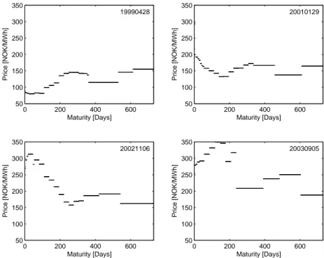
Fig. 1. The term structure of electricity prices observed on four different days: April 28, 1999, January 29, 2001, November 6, 2002, and September 5, 2003.
minimum of 4 contracts are traded each week. New contracts are introduced every fourth Monday. Block futures contracts are no longer traded. They had 4 week (28 day) delivery periods. Each year was divided into 13 block contracts, 10 of which were traded simulta- neously. This system had the advantage of all block contracts having the same number of delivery hours, but the disadvantage of the delivery periods not matching calendar months.
To avoid this, and to offer products more similar to contracts being traded at other ex- changes, block contracts were replaced in 2003 by monthly futures with delivery periods corresponding to calendar months. Monthly futures are not traded in the month prior to delivery; at that time weekly futures are available. Each month one contract expires and a new one is introduced.
Seasonal and annual contracts are forward-style instruments. However, until 1999 the former were marked-to-market like weekly and block futures contracts. Also their contract specifications have changed from a seasonal to a quarterly structure. Previously each year was divided into three seasons: V1 – late winter (January 1 – April 30), S0 – summer (May 1 – September 30) and V2 – early winter (October 1 – December 31). The first quarterly seasonal contracts were listed in 2004 for each quarter of the year 2006. Finally, annual contracts have delivery periods of one year. In the analyzed time interval (1999-2004) they spanned a period of three years; currently they reach as far as 6 years into the future. Annual contracts have a delivery period of 24×365 = 8760 hours (or 8784 hours in leap years).
Monthly futures, and all contracts introduced in 2003 and later, are denominated in EUR (previously NOK). In order to unify the currency we recalculated all prices to NOK using spot exchange rates from the Reuters EcoWin database. In the case when futures and forward contracts overlapped for some delivery period we took the futures contract prices (i.e. the contract closer to delivery) for this period.
The term structure for four randomly selected days across the sample are displayed in Figure 1. Although only one price is quoted per contract it corresponds to some prespecified delivery period and, therefore, the term structure is a piecewise constant curve. The delivery periods are shorter near expiry, which results in a more split curve and higher variation for nearby maturities. Note that the forward curve exhibits different shapes on different days, which suggests that the term structure of electricity prices is a highly dynamic object.
Moreover, it can be observed that the curve is seasonal or even sinusoidal with a period of approximately one year.
3. Factor models
The object of factor analysis is to describe fluctuations over time in a set of variables through those experienced by a small set of factors. Observed variables are assumed to be linear combinations of the unobserved factors, with the factors being characterized up to scale and rotation transformations. For instance, a J-dimensional vector of observations Yt= (Yt,1, ..., Yt,J) can be represented as an (orthogonal)L-factor model
Yt,j =m0,j +Zt,1m1,j+...+Zt,LmL,j+εt,j, (1) whereZt,l are common factors, the coefficientsml,j are factor loadings andεt,j are specific factors (or errors) which explain the residual part (Pe˜na and Box, 1987). The index t = 1, ..., T represents the time evolution of the observed vector of variables.
The most important feature of factor models in finance is that they allow for reducing the dimensionality of a set of assets in a portfolio, leading to much more parsimonious and efficient risk management tools (of course, only if L ≪ J). In the context of curve modeling, factor models have gained popularity in the 1990s with the works of Litterman and Scheinkman (1991) and Steeley (1990). These authors used factor analysis (more precisely:
PCA) to extract common (latent) factors driving yield curves in different countries and periods. They concluded (and this was later confirmed by other authors) that three principal components – interpreted as level, slope and curvature – were enough to almost fully (>95%) explain the dynamics of the term structure of interest rates; note, that such a parsimonious description is not as accurate in electricity markets (Koekebakker and Ollmar, 2005, Weron, 2006).
In this paper we work in a semiparametric factor model setup and, following Borak et al.
(2007), modify the basic model (1) by incorporating observable covariatesXt,j. The factor loadings ml,j are now generalized to functions of the covariates and the model takes the form:
Yt,j=m0(Xt,j) + XL
l=1
Zt,lml(Xt,j) +εt,j. (2) The functionsml(·) are nonparametric, while the factorsZt,lrepresent the parametric part, hence the name dynamic semiparametric factor model (DSFM); for a recent review of non- and semiparametric models see H¨ardle et al. (2004). The model can be regarded as a re- gression model with embedded time evolution. Additionally, the regularity of the multi- dimensional time series may be omitted by allowing time dependentJ, sayJt.
The DSFM was introduced by Fengler et al. (2007) in the context of modeling implied volatility surfaces of DAX options. Borak et al. (2007) further refined the original algorithms by implementing a series based estimator instead of a kernel smoother. They also showed
asymptotic equivalence of the covariance based inference on estimated and true unobservable factors.
In the context of electricity markets, Yt,j denotes the observed forward electricity price observed on day t= 1, . . . , T for delivery in periodj = 1, . . . , Jt. As the number of traded futures and forward contracts varies throughout the year (see Section 2)Jtis not a constant, but can take one of a few values. The corresponding maturity date or time point we denote by Xt,j. Since delivery of electricity does not take place at some instant, but rather continuously over a time interval,Xt,j represents the midpoint of the delivery periodj.
When calibrating a factor model of the form (2) two major issues arise. First, there is the problem of uniqueness. The signs ofZt,l andmlcannot be identified as only their product appears in the formula, while certain linear transformations, e.g. rotation, yield the same model for different functions. Moreover, one can add a constantctoZt,land subtractc·ml(·) fromm0(·) to get the same model. A possible choice for the identification procedure (and we use it here) is to set the estimatesmbl ofml to be orthogonal and order them with respect to the variation ofPT
t=1Zˆt,l2, then center the estimatesZbt,l ofZt,l to have zero mean. This ordering makes the DSFM similar to PCA. What makes them different is the calibration scheme. The DSFM is more flexible in this respect. It minimizes the squared residua (or maximizes the in-sample fit with respect to some score function), while a factor model estimated through PCA maximizes the expected variance (Ramsay and Silverman, 1997).
Second, there is the problem of irregularity. Since traded futures and forward contracts can have delivery periods of significantly different lengths, the estimation procedure should value individual prices differently. Certainly, the price of an annual forward contract should impact a larger portion of the curve than the price of a weekly futures contract. One possible solution would be to weigh the prices relative to the length of the delivery period. While for low order (L= 3) models this procedure generally performs satisfactorily, for larger models (L≥4) the loading functionsml(·) become very volatile since the fit is penalized only if it deviates in the midpointsXt,j of the delivery periods. The second solution to this problem becomes obvious if we rewrite formula (2) in a functional form:
yt(τ) = XL
l=0
Zt,lml(τ) +εt(τ), (3)
whereZt,0= 1. Now,yt(·),ml(·) andεt(·) are functions of maturityτ, a continuous variable.
We can discretizeτ and perform the estimation on a regular gridX1, ..., XJ, independently of the observation timet(naturally, the grid has to be fine enough to adequately represent all delivery periods). In this way, forward contracts with longer delivery periods will auto- matically have more impact on the curve. Then the DSFM of order L takes the following form:
Yt,j=m0(Xj) + XL
l=1
Zt,lml(Xj) +εt,j. (4) The loading functions ml(·) need not take a specific form, however, in this study we linearize them with B-splines (for details on B-splines we refer to the monograph of de Boor, 2001). Namely we let
ml(Xj) = XK
k=1
al,kψk(Xj), (5)
whereKis the number of knots,ψk(·) are the splines andal,kare the appropriate coefficients.
The estimation procedure searches through all loading functions ml and time seriesZt,l
minimizing the following least squares (LS) criterion:
XT
t=1
XJ
j=1
( Yt,j−
XL
l=0
Zt,l XK
k=1
al,kψk(Xj) )2
. (6)
Note that, conditional on Zt,l, the minimizer al,k is the traditional LS estimator. Hence, knowingal,k reduces (6) toT separate LS problems.
The calibration proceeds as follows. First, we set the initial estimateZbt,l(0) to be equal to a white noise sequence of appropriate length. Next, taking this initial estimate as given we find the initial estimateba(0)l,k. Then we proceed iteratively switching fromZbt,ltobal,kand vice versa until convergence is reached. Although the algorithm is not guarantied to converge, in this study we have not suffered major problems related to this issue. For more details on the calibration procedure we refer to Borak et al. (2007).
4. Empirical evidence
Now we are ready to calibrate the DSFM to the dataset described in Section 2, i.e. futures and forward contracts traded at Nord Pool in the period January 4, 1999 – July 6, 2004.
Only models of order L = 3,4,5,6 are considered. By adding more factors we obtain a (generally) better fit, at the cost of universality (robustness) and parsimony of the model (and consequently: computational speed). We have decided not to execute this option and consider six factor models at most. At the other end, using models with less than three factors leads to a very poor description of the term structure.
The calibration is performed in the moving window spirit, with the window length being equal toT= 500 business days (or roughly two years). In each step we shift our sample by one day, discarding the oldest observation and including a new day. The first window starts on January 4, 1999 and ends on December 29, 2000, the last covers the period July 2, 2002 – July 6, 2004. In this way, we obtain 862 (= 1361−499) DSFM fits for each of the model sizes (L = 3,4,5,6). Note, that the term structure on some days can have several DSFM representations, in particular all days in the period December 29, 2000 – July 2, 2002 have 500 different fits (as each of them falls into 500 windows). The differences for neighboring windows are negligible, but windows that are far apart can lead to visually different fits.
The time grid used consists of J = 1432 equidistant points, Xj = 15,15.5,16, ...,730, representing time to maturity in days. The first two weeks are omitted due to very high volatility at the short end of the forward curve. The very long end of the curve (more than 2 years from today) is not analyzed since for such distant maturities only annual contracts are traded.
For the basis functionsψk(·), 19 cubic B-splines evaluated on equidistant knots are used.
The number of spline functions is related to the mean number of observations per day and as long as the splines are of degree 1 or more (i.e. at least linear) we find the placement of the knots and the selection ofKof minor importance to the accuracy of the fit.
Calibration results forL= 3 and prices covering the period June 3rd, 1999 – June 17th, 2003 are displayed in Figure 2. The period is divided into two adjacent time intervals (500 day windows): until June 11th, 2001 and after (and including) June 12th, 2001. The structure of the loading functions seems to be stable throughout the sample, however, the time series
b
Zt,l vary considerably between the periods. The functions mb1 are relatively flat and could be interpreted as overall level changes. Their absolute values decrease with maturity, which
Jan00 Jan01
−3000
−2000
−1000 0 1000 2000 3000
200 400 600
−0.1
−0.05 0 0.05 0.1
Jan02 Jan03
−3000
−2000
−1000 0 1000 2000 3000
200 400 600
−0.1
−0.05 0 0.05
0.1 m1
m2 m3 m1
m2 m3
Zt,1 Zt,2 Zt,3 Zt,1
Zt,2 Zt,3
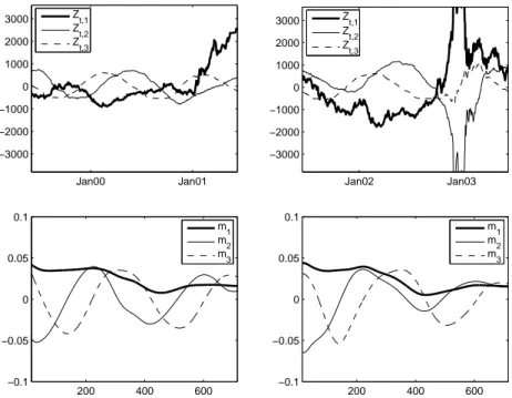
Fig. 2. Estimated time seriesZbt,l(upper panels) and loadingsmbl(Xj) (lower panels) for the DSFM of order L= 3 andXj= 15,15.5,16, ...,730 days (the functionsmb0 are not displayed). The data sample covering the period June 3rd, 1999 – June 17th, 2003 is divided into two adjacent time intervals: until June 11th, 2001 (left panels) and after (and including) June 12th, 2001 (right panels). The structure of the loading functions seems to be stable throughout the sample, however, the time seriesZbt,lvary considerably between the periods.
coincides with the highest volatility at the short end of the curve and the lowest at the long end. The factor Zbt,1 reflects then the trend of the entire term structure. The second and third elements of the model exhibit periodic behavior, both in spacial loading functions and time dependent factors. The period is approximately one year and the factors can be interpreted as seasonal adjustments of the curve, required for adequate representation of the curve throughout the whole year. There are some deviations from this behavior but the presented pattern, namely one trend factor and two seasonal factors, dominates in the analyzed dataset.
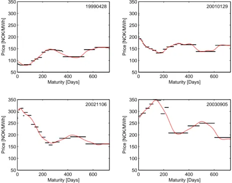
In Figures 3 and 4 we present DSFM fits to the term structure of electricity prices observed on the same four days as in Figure 1. The fit forL= 6 in not necessarily better than forL= 3, but certainly more closely follows the quoted prices. Compared to fits obtained within the
‘maximum smoothness’ principle (Koekebakker and Ollmar, 2005, Benth et al., 2007), the DSFM approach yields less pronounced seasonality in the far end of the curve. Compared to the results of Fleten and Lemming (2003), the obtained curves are smoother and less closely follow the quoted prices (at least forL= 3, see Fig. 3).
As far as the goodness-of-fit is concerned, there are two standard loss functions to be considered – one based on the L1 norm, the other on the L2 norm. The former tends to disclose more details, hence we use it here. It is defined by:
ǫL1 = XT
t=1
XJ
j=1
|Yt,j−M odel(Xj)|. (7)
0 200 400 600 50
100 150 200 250 300 350
19990428
Price [NOK/MWh]
Maturity [Days]
0 200 400 600
50 100 150 200 250 300 350
20010129
Price [NOK/MWh]
Maturity [Days]
0 200 400 600
50 100 150 200 250 300 350
20021106
Price [NOK/MWh]
Maturity [Days]
0 200 400 600
50 100 150 200 250 300 350
20030905
Price [NOK/MWh]
Maturity [Days]
Fig. 3. The term structure of electricity prices and the estimated forward curves (forL= 3) observed on the same four days as in Figure 1.
0 200 400 600
50 100 150 200 250 300 350
19990428
Price [NOK/MWh]
Maturity [Days]
0 200 400 600
50 100 150 200 250 300 350
20010129
Price [NOK/MWh]
Maturity [Days]
0 200 400 600
50 100 150 200 250 300 350
20021106
Price [NOK/MWh]
Maturity [Days]
0 200 400 600
50 100 150 200 250 300 350
20030905
Price [NOK/MWh]
Maturity [Days]
Fig. 4. The term structure of electricity prices and the estimated forward curves (forL= 6) observed on the same four days as in Figure 1. The fit in not necessarily better than forL= 3 (see Fig. 3), but certainly more closely follows the quoted prices.
0 100 200 300 400 500 600 700 800 900 1000 0.5
1 1.5
2x 10⁴
DSFM(3)
DSFM(4)
DSFM(5)
DSFM(6)
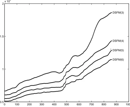
Fig. 5. In-sample error ǫL
1 as a function of time for different model sizes (L= 3,4,5,6). The first data point (#1) corresponds to a window starting on January 4, 1999 and ending on December 29, 2000, the last (#862) to a window covering the period July 2, 2002 – July 6, 2004.
Note, that the forward curve resulting from the DSFM is a smooth function, while the original prices have a piecewise constant shape. Obviously, the error will be non-negligible no matter what period is analyzed.
The in-sample error as function of time is presented in Figure 5. Clearly the models with more factors give a better fit, although for models calibrated to price quotations in the beginning of the dataset this feature is less pronounced. For all L we observe an upward trend, which implies that models with the same number of factors yield a much better fit in the first part of the sample than in the second. In particular, this is visible forL = 3.
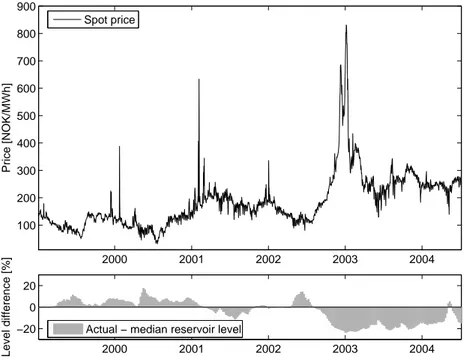
A significant loss of accuracy can be observed roughly in the middle of the sample, ca. for window number 450 covering the period October 18, 2000 – October 31, 2002. The reason for this were the weather conditions. A dry autumn and an early and severe winter 2002/2003 resulted in extremely low hydropower reservoir levels – lowest since the commencement of exchange trading at Nord Pool in 1993. With more than 50% of all power generation in the Nordic countries from hydropower, this gave rise to price levels never seen before in this market, see Figure 6. The average system price for 2003 was 291 NOK/MWh, compared with an average of 158 NOK/MWh for the 1996-2002 period. The highest average daily system price recorded between 1993 and 2007 was set on January 6, 2003: 831 NOK/MWh (see www.nordpool.com). High prices were accompanied by an unprecedented market volatility.
Futures contracts reached prices that, for a brief time, exceeded prices at the spot market.
These abnormal market conditions persisted throughout 2004, resulting in very volatile and less predictable spot and forward prices. In fact, looking at Figure 6, we can observe that the deviations from the ‘normal’, seasonal spot price behavior of the years 1999-2000 increase over time. Obviously this leads to a steady increase of the in-sample error ǫL1 over time
2000 2001 2002 2003 2004 100
200 300 400 500 600 700 800 900
Price [NOK/MWh]
2000 2001 2002 2003 2004
−20 0 20
Level difference [%]
Spot price
Actual − median reservoir level
Fig. 6.Top panel: Daily average spot system prices in the period January 4, 1999 – July 6, 2004.Bottom panel: The difference (in percent) between the actual and median (for 1990-2003) reservoir levels in Norway.
As long as the actual level is above the median, the spot prices behave ‘normally’. When the actual level substantially drops below the median the prices increase, as in spring 2001 and autumn 2002.
(Fig. 5), independent of the model sizeL.
5. Conclusions
In this paper we have introduced the dynamic semiparametric factor model (DSFM) for modeling electricity forward curves. The model utilizes a parsimonious factor representation – a linear combination of nonparametric loading functions (linearized with B-splines) and parametrized common factors. It is calibrated within a least squares iterative scheme. The biggest advantage of the DSFM approach is that it not only leads to smooth, seasonal electricity forward curves, but also to a parsimonious factor representation of the curve.
Using a database of financial contracts traded at the Nordic power exchange Nord Pool in the years 1999-2004, we have provided empirical evidence that the DSFM is an efficient modeling tool. It turns out that a parsimonious 3-factor representation yields reasonable fits throughout the whole sample. More complex models (with more factors) lead to more accurate in-sample fits (e.g. a 6-factor model is better by roughly 30%) at the cost of universality (robustness) and computational speed. Compared to fits obtained within the
‘maximum smoothness’ principle (Koekebakker and Ollmar, 2005, Benth et al., 2007), the DSFM approach yields less pronounced seasonality in the far end of the curve. Compared to the results of Fleten and Lemming (2003), the obtained curves are smoother and less closely follow the quoted prices.
The structure of the loading functions has been found to be stable throughout the sample.
This result shows that incorrect specification of the loading functions is moderately harmful,
as long as they resemble the functions in Figure 2. We believe that this can be an insightful guidance for parametric factor representations of electricity forward curves. The functions
b
m1are relatively flat and could be interpreted as overall level changes. Their absolute values decrease with maturity, which coincides with the highest volatility at the short end of the curve and the lowest at the long end. The first factorZbt,1reflects then the trend of the entire term structure. The second and third elements of the model exhibit periodic behavior, both in spacial loading functions and time dependent factors. The period is approximately one year and the factors can be interpreted as seasonal adjustments of the curve, required for adequate representation of the curve throughout the whole year.
References
Adams, K.J., van Deventer, D. R. (1994). Fitting yield curves and forward rate curves with maximum smoothness,Journal of Fixed Income 4, 52-62.
Benth, F.E., Koekebakker, S., Ollmar, F. (2007). Extracting and applying smooth forward curves from average-based commodity contracts with seasonal variation,Journal of Derivatives, Fall, 52-66.
Borak, S., H¨ardle, W., Mammen, E., Park, B. (2007). Time series modelling with semiparametric factor dynamics,Discussion Paper SfB 649, Humboldt-Universit¨at zu Berlin.
Bunn, D.W., ed. (2004).Modelling Prices in Competitive Electricity Markets, Wiley, Chichester.
De Boor, C. (2001).A Practical Guide to Splines, Springer-Verlag, New York.
Fengler, M.R., H¨ardle, W., Mammen, E. (2007). A semiparametric factor model for implied volatility surface dynamics,Journal of Financial Econometrics5(2), 189-218.
Fielden, S. (2005). Shopping for curves,Energy Risk, March, 122-124.
Fleten, S.E., Lemming, J. (2003). Constructing forward price curves in electricity markets,Energy Economics 25, 409-424.
Hagan, P.S., West, G. (2006). Interpolation methods for curve construction,Applied Mathematical Finance 13(2), 89-129.
Harris, C. (2006).Electricity Markets: Pricing, Structures and Economics,Wiley, Chichester.
H¨ardle, W., M¨uller, M., Sperlich, S., Werwatz, A. (2004). Nonparametric and Semiparametric Models, Springer Verlag, Heidelberg.
Koekebakker, S., Ollmar, F. (2005). Forward curve dynamics in the Nordic electricity market,Managerial Finance 31(6), 73-94.
Litterman, R., Scheinkman, J. (1991). Common Factors Affecting Bond Returns,Journal of Fixed Income 1, 62-74.
Pe˜na, D., Box, E. P. (1987). Identifying a simplifying structure in time series, Journal of the American Statistical Association82, 836-843.
Ramsay, J.O., Silverman, B.W. (1997).Functional Data Analysis, Springer-Verlag, Berlin.
Steeley, J.M. (1990). Modeling the dynamics of the term structure of interest rates,Economic and Social Review 21(4), 337-661.
Weron, R. (2006).Modeling and Forecasting Electricity Loads and Prices: A Statistical Approach, Wiley, Chichester.
SFB 649 Discussion Paper Series 2008
For a complete list of Discussion Papers published by the SFB 649, please visit http://sfb649.wiwi.hu-berlin.de.
001 "Testing Monotonicity of Pricing Kernels" by Yuri Golubev, Wolfgang Härdle and Roman Timonfeev, January 2008.
002 "Adaptive pointwise estimation in time-inhomogeneous time-series models" by Pavel Cizek, Wolfgang Härdle and Vladimir Spokoiny,
January 2008.
003 "The Bayesian Additive Classification Tree Applied to Credit Risk Modelling" by Junni L. Zhang and Wolfgang Härdle, January 2008.
004 "Independent Component Analysis Via Copula Techniques" by Ray-Bing Chen, Meihui Guo, Wolfgang Härdle and Shih-Feng Huang, January 2008.
005 "The Default Risk of Firms Examined with Smooth Support Vector Machines" by Wolfgang Härdle, Yuh-Jye Lee, Dorothea Schäfer and Yi-Ren Yeh, January 2008.
006 "Value-at-Risk and Expected Shortfall when there is long range dependence" by Wolfgang Härdle and Julius Mungo, Januray 2008.
007 "A Consistent Nonparametric Test for Causality in Quantile" by Kiho Jeong and Wolfgang Härdle, January 2008.
008 "Do Legal Standards Affect Ethical Concerns of Consumers?" by Dirk Engelmann and Dorothea Kübler, January 2008.
009 "Recursive Portfolio Selection with Decision Trees" by Anton Andriyashin, Wolfgang Härdle and Roman Timofeev, January 2008.
010 "Do Public Banks have a Competitive Advantage?" by Astrid Matthey,
January 2008.
011 "Don’t aim too high: the potential costs of high aspirations" by Astrid Matthey and Nadja Dwenger, January 2008.
012 "Visualizing exploratory factor analysis models" by Sigbert Klinke and Cornelia Wagner, January 2008.
013 "House Prices and Replacement Cost: A Micro-Level Analysis" by Rainer Schulz and Axel Werwatz, January 2008.
014 "Support Vector Regression Based GARCH Model with Application to Forecasting Volatility of Financial Returns" by Shiyi Chen, Kiho Jeong and Wolfgang Härdle, January 2008.
015 "Structural Constant Conditional Correlation" by Enzo Weber, January 2008.
016 "Estimating Investment Equations in Imperfect Capital Markets" by Silke Hüttel, Oliver Mußhoff, Martin Odening and Nataliya Zinych, January 2008.
017 "Adaptive Forecasting of the EURIBOR Swap Term Structure" by Oliver Blaskowitz and Helmut Herwatz, January 2008.
018 "Solving, Estimating and Selecting Nonlinear Dynamic Models without the Curse of Dimensionality" by Viktor Winschel and Markus Krätzig,
February 2008.
019 "The Accuracy of Long-term Real Estate Valuations" by Rainer Schulz, Markus Staiber, Martin Wersing and Axel Werwatz, February 2008.
020 "The Impact of International Outsourcing on Labour Market Dynamics in Germany" by Ronald Bachmann and Sebastian Braun, February 2008.
021 "Preferences for Collective versus Individualised Wage Setting" by Tito Boeri and Michael C. Burda, February 2008.
SFB 649, Spandauer Straße 1, D-10178 Berlin http://sfb649.wiwi.hu-berlin.de
This research was supported by the Deutsche
022 "Lumpy Labor Adjustment as a Propagation Mechanism of Business Cycles" by Fang Yao, February 2008.
023 "Family Management, Family Ownership and Downsizing: Evidence from S&P 500 Firms" by Jörn Hendrich Block, February 2008.
024 "Skill Specific Unemployment with Imperfect Substitution of Skills" by Runli Xie, March 2008.
025 "Price Adjustment to News with Uncertain Precision" by Nikolaus Hautsch, Dieter Hess and Christoph Müller, March 2008.
026 "Information and Beliefs in a Repeated Normal-form Game" by Dietmar Fehr, Dorothea Kübler and David Danz, March 2008.
027 "The Stochastic Fluctuation of the Quantile Regression Curve" by Wolfgang Härdle and Song Song, March 2008.
028 "Are stewardship and valuation usefulness compatible or alternative objectives of financial accounting?" by Joachim Gassen, March 2008.
029 "Genetic Codes of Mergers, Post Merger Technology Evolution and Why Mergers Fail" by Alexander Cuntz, April 2008.
030 "Using R, LaTeX and Wiki for an Arabic e-learning platform" by Taleb Ahmad, Wolfgang Härdle, Sigbert Klinke and Shafeeqah Al Awadhi, April 2008.
031 "Beyond the business cycle – factors driving aggregate mortality rates"
by Katja Hanewald, April 2008.
032 "Against All Odds? National Sentiment and Wagering on European Football" by Sebastian Braun and Michael Kvasnicka, April 2008.
033 "Are CEOs in Family Firms Paid Like Bureaucrats? Evidence from Bayesian and Frequentist Analyses" by Jörn Hendrich Block, April 2008.
034 "JBendge: An Object-Oriented System for Solving, Estimating and Selecting Nonlinear Dynamic Models" by Viktor Winschel and Markus Krätzig, April 2008.
035 "Stock Picking via Nonsymmetrically Pruned Binary Decision Trees" by Anton Andriyashin, May 2008.
036 "Expected Inflation, Expected Stock Returns, and Money Illusion: What can we learn from Survey Expectations?" by Maik Schmeling and Andreas Schrimpf, May 2008.
037 "The Impact of Individual Investment Behavior for Retirement Welfare:
Evidence from the United States and Germany" by Thomas Post, Helmut Gründl, Joan T. Schmit and Anja Zimmer, May 2008.
038 "Dynamic Semiparametric Factor Models in Risk Neutral Density Estimation" by Enzo Giacomini, Wolfgang Härdle and Volker Krätschmer,
May 2008.
039 "Can Education Save Europe From High Unemployment?" by Nicole Walter and Runli Xie, June 2008.
042 "Gruppenvergleiche bei hypothetischen Konstrukten – Die Prüfung der Übereinstimmung von Messmodellen mit der Strukturgleichungs- methodik" by Dirk Temme and Lutz Hildebrandt, June 2008.
043 "Modeling Dependencies in Finance using Copulae" by Wolfgang Härdle, Ostap Okhrin and Yarema Okhrin, June 2008.
044 "Numerics of Implied Binomial Trees" by Wolfgang Härdle and Alena Mysickova, June 2008.
045 "Measuring and Modeling Risk Using High-Frequency Data" by Wolfgang Härdle, Nikolaus Hautsch and Uta Pigorsch, June 2008.
046 "Links between sustainability-related innovation and sustainability management" by Marcus Wagner, June 2008.
SFB 649, Spandauer Straße 1, D-10178 Berlin http://sfb649.wiwi.hu-berlin.de
This research was supported by the Deutsche
Forschungsgemeinschaft through the SFB 649 "Economic Risk".
SFB 649, Spandauer Straße 1, D-10178 Berlin http://sfb649.wiwi.hu-berlin.de
This research was supported by the Deutsche
047 "Modelling High-Frequency Volatility and Liquidity Using Multiplicative Error Models" by Nikolaus Hautsch and Vahidin Jeleskovic, July 2008.
048 "Macro Wine in Financial Skins: The Oil-FX Interdependence" by Enzo Weber, July 2008.
049 "Simultaneous Stochastic Volatility Transmission Across American Equity Markets" by Enzo Weber, July 2008.
050 "A semiparametric factor model for electricity forward curve dynamics" by Szymon Borak and Rafał Weron, July 2008.