Lorenzo Zampieri1 and Helge F. Goessling1
1Alfred Wegener Institute, Helmholtz Centre for Polar and Marine Research, Bremerhaven, Germany
Abstract
To counteract global warming, a geoengineering approach that aims at intervening in the Arctic ice-albedo feedback has been proposed. A large number of wind-driven pumps shall spread seawater on the surface in winter to enhance ice growth, allowing more ice to survive the summer melt.We test this idea with a coupled climate model by modifying the surface exchange processes such that the physical effect of the pumps is simulated. Based on experiments with RCP 8.5 scenario forcing, we find that it is possible to keep the late-summer sea ice cover at the current extent for the next∼60 years. The increased ice extent is accompanied by significant Arctic late-summer cooling by∼1.3 K on average north of the polar circle (2021–2060). However, this cooling is not conveyed to lower latitudes. Moreover, the Arctic experiences substantial winter warming in regions with active pumps. The global annual-mean near-surface air temperature is reduced by only 0.02 K (2021–2060). Our results cast doubt on the potential of sea ice targeted geoengineering to mitigate climate change.
1. Introduction
The declining trend of the Arctic sea ice extent (Comiso, 2011; Kay et al., 2011; Lindsay & Schweiger, 2015;
Stroeve et al., 2012), caused mainly by anthropogenic greenhouse gas emissions (Notz & Stroeve, 2016), is expected to continue. Projections based on climate models foresee a largely ice-free Arctic Ocean in late summer around the mid-21st century in the business-as-usual emission scenario (Intergovernmental Panel on Climate Change, 2014; Jahn, 2018; Niederdrenk & Notz, 2018; Notz & Stroeve, 2018). The replacement of the highly reflective ice cover by the dark ocean has been described as one of the most severe positive feed- backs in the climate system (Manabe & Stouffer, 1980) and contributes to the Arctic warming amplification (Pithan & Stouffer, 2014).
The Paris Agreement stipulates the reduction of greenhouse gas emissions to keep global warming well below 2◦C (Cornwall, 2015; United Nations, 2015). However, even if all national commitments to curb emissions will be implemented, the 2 C target will likely be exceeded significantly (Rogelj et al., 2016).◦ The discussion around alternative approaches based on climate engineering—the anthropogenic large-scale modification of the Earth's climate to mitigate global warming (Bellamy et al., 2017; Keith, 2001; Talberg et al., 2018)—is highly controversial (Blackstock & Long, 2010; Givens, 2018; Hamilton, 2013). Neverthe- less, with the prospect of insufficient emission reductions, the scientific examination of climate engineering strategies appears advisable.
Several climate engineering approaches that focus on the Arctic sea ice cover and the positive ice-albedo feedback have been proposed (Cvijanovic et al., 2015; Desch et al., 2017; Field et al., 2018; Mengis et al., 2016;
Seitz, 2011). The Arctic Ice Management (AIM) strategy put forward in Desch et al. (2017, D17 hereafter), which attracted the attention of the scientific community and the media alike (rated within the top 5% of all research output; Altmetric Attention Score, 2017), entails the large-scale employment of wind-driven pumps that spread seawater on the ice surface in the winter months. The sea ice and the snow that is accumulated over it are materials with low thermal conductivity compared to the ocean water. During the freezing season, even a thin layer of sea ice limits the heat flux from the warmer ocean to the cooler atmosphere considerably (Trodahl et al., 2001), reducing the growth of additional sea ice. The AIM approach aims to bypass the thermally insulating effect of sea ice, allowing thereby more ice to grow thick enough during winter to withstand the summer melt (Figure 1).
Special Section:
The Arctic: An AGU Joint Special Collection
Lorenzo Zampieri and Helge F. Goessling contributed equally to this work.
Key Points:
• Sea ice targeted geoengineering allows to keep the late-summer sea ice cover at the current extent for the next∼60 years
• The Arctic summer cooling is not conveyed to lower latitudes and comes at the price of Arctic winter warming
• Our results cast doubt on the potential of Arctic Ice Management to mitigate climate change
Supporting Information:
• Supporting Information S1
Correspondence to:
L. Zampieri and H. F. Goessling, lorenzo.zampieri@awi.de;
helge.goessling@awi.de
Citation:
Zampieri, L., & Goessling, H. F.
(2019). Sea ice targeted
geoengineering can delay Arctic sea ice decline but not global warming.
Earth's Future.7
Received 9 APR 2019 Accepted 6 OCT 2019
©2019. The Authors.
This is an open access article under the terms of the Creative Commons Attribution License, which permits use, distribution and reproduction in any medium, provided the original work is properly cited.
Published online 05 DEC 2019 029/2019EF001230 1
https://doi.org/10.
,1296
1306.
–
Earth’s Future
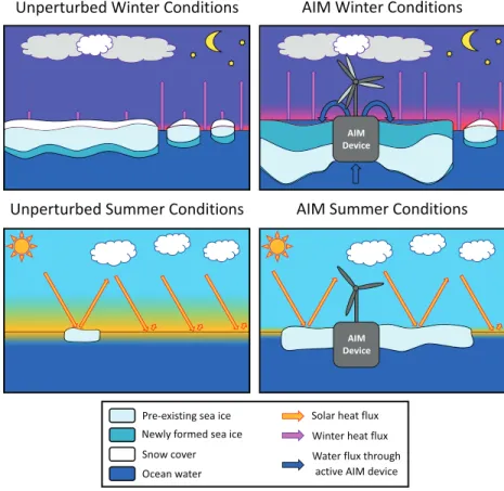
10.1029/2019EF001230Figure 1.Idealized representation of the 21st century sea ice system with and without Arctic Ice Management (AIM).
In unperturbed winter conditions (top left) the sea ice and snow act as insulator reducing the heat flux from the warmer ocean to the much colder atmosphere. The sea ice growth takes place mostly at the ice-ocean interface and is relatively slow (dark blue fraction of the ice floes). By summer (bottom left) most of the ice has melted, leading to an ice-free Arctic Ocean in the second half of the century and amplifying the warming through the ice-albedo feedback (yellow fraction of ocean). In AIM conditions (top right) ocean water is pumped onto the ice, leading to larger heat flux and rapid ice growth at the surface. More ice withstands the summer melt (bottom right) and increases the surface albedo.
Based on simple thermodynamical arguments and observations from an ice mass balance buoy in the Beau- fort Sea, D17 estimate that∼1.4 m of seawater would need to be pumped onto the ice to generate∼1.0 m of extra ice thickness over the course of one winter at a typical location in the Arctic Ocean. They envisage the deployment of∼10 million devices, each comprising a wind turbine, a pump, a water tank, and a delivery system that distributes the water over an area of 0.1 km2. D17 calculate that 1 m extra ice thickness would lead to a shift of the local melt date by∼15 weeks (3 weeks per 0.2 m). They argue that it might be possible to maintain a large part of the usually seasonal ice zone throughout the summer by appropriate annual repo- sitioning and/or reseeding of the AIM array. Considering associated albedo changes, D17 calculate a global annual-mean shortwave radiative cooling by up to 0.14 W/m2. This is about half of the estimate by Hudson (2011) for the global annual-mean forcing associated with a virtually ice-free Arctic summer (0.3 W/m2) and a significant fraction of the current anthropogenic radiative forcing by∼1 W/m2.
Considering energy requirements, economical demands, and technical challenges, D17 conclude that such a major undertaking seems indeed feasible. However, the question is left open what the quantitative response of the Arctic as well as the global climate system would be. It is also unclear whether the local thermody- namic considerations can be scaled up to the whole Arctic. For example, the large-scale exposure of relatively warm ocean water is expected to generate positive near-surface temperature anomalies. Because the surface turbulent heat fluxes are proportional to the surface temperature gradient (Serreze et al., 2007; Wallace &
Hobbs, 2006), increased winter temperatures might induce a negative feedback that dampens the additional ice growth. Complex climate models that simulate the relevant physics, including the general circulations of the atmosphere and the ocean, can provide answers.
Here we use the Alfred Wegener Institute Climate Model (AWI-CM; Danilov et al., 2015; Rackow et al., 2016;
Sidorenko et al., 2015) to study the efficacy of AIM and the response of the climate system, in the Arctic and beyond. To this end we modify the parameterization of the surface heat and mass fluxes in ice-covered ocean regions north of the polar circle (∼ 66.5◦N) such that the effect of the AIM devices is simulated.
The modification is activated during the Arctic winter from 21 October to 21 March from 2020 onward.
The strength of the modification is modulated with two parameters that affect the large-scale spatial extent and the local efficiency of the pumps. A sensitivity analysis with respect to these parameters is followed by a more detailed analysis based on ensemble simulations (4×unperturbed and 4×AIM) with RCP 8.5 scenario forcing until 2100. Moreover, we analyze the effect of an abrupt suspension of AIM in 2030 to test its reversibility.
2. Results
2.1. Regulating the Strength of AIM
The impact of AIM depends on the strength of the modification applied. In the real world, this would depend on the number and spatial distribution of the deployed AIM devices, as well as their efficiency in distribut- ing the ocean water over the surrounding sea ice. To start with, we have performed a simulation where a liquid layer is maintained over the whole ice cover, allowing us to determine an upper bound for the impact of AIM on the ice and on the global climate. This extreme scenario should be regarded as an idealized case to test the response of the climate system to AIM. In this experiment the mean Arctic ice thickness increases almost linearly by∼2.1 m per year from 2020 to 2030 (the historical 1850–2000 annual-mean value is∼1.8 m).
Thereafter the thickness growth slows down until the mean thickness levels off around 65 m from 2080 onward, corresponding to a pan-Arctic ice volume of∼900×103km3(supporting information Figure S1, right). The ice extent attains values around 15×106km2in late winter (February) and 13.5×10⁶km2in late summer (September; Figure S1, left). This implies almost a doubling of the late-summer sea ice extent compared to historical conditions (1850–2000). The ice thickness and extent stop growing due to the grad- ual warming by increasing greenhouse gas concentrations and, for the same reason, would start to decline beyond 2100 despite AIM.
The near-surface temperature response in this extreme case is profound: Averaged over 2021–2060 north of 66.5◦N, the Arctic is colder by∼5.2 K in September, compared to the four-member ensemble of unperturbed runs without AIM, but warmer by∼10.6 K in February when the pumps are active (Figure S2, top). The northern middle latitudes (30–60◦N), however, are warmer by 0.5–1.0 K throughout the year. This implies that the radiative cooling from the increased albedo is not strong enough to (over)compensate the effect from the direct Arctic winter warming which is transported to lower latitudes by atmospheric advection and persists there in the ocean mixed layer throughout the year. (The September warming of the northern middle latitudes tends to be present already after a single AIM season [Figure S2; 2020], which is not compatible with the typical time scale for oceanic transport.) The results raise the question whether a more moderate implementation of AIM, where pumps are employed only where they are needed to make the ice thick enough to survive the summer melt, might be better suited to generate an overall cooling. A weaker AIM implementation is also more realistic given that it seems unlikely that the AIM devices would be able to maintain a closed cover of liquid water and also in regard to the number of devices required: The extreme case corresponds to more than 10 times the number of devices envisaged by D17.
We have thus introduced two parameters that affect the large-scale spatial extent and the local efficiency of the AIM devices: The Global Modulation Parameter (GMP) determines an ice thickness threshold beyond which the pumps are deactivated. Thereby the modification is active only in regions with relatively thin ice, where extra ice thickness can reduce the chances of the ice to melt completely over the course of the subsequent summer. In contrast, the Local Modulation Parameter (LMP) determines which fraction of the ice surface in model grid cells with active pumps is covered by water. The LMP represents the spatial density of AIM devices as well as their efficiency to maintain a liquid layer.
To explore the impact of the two parameters, we have conducted nine simulations from 2020 to 2040 by combining three GMP values (1, 2, and 3 m) with three LMP values (25%, 50%, and 75%; Figures 2 and S3).
Averaged over all 20 years, the March sea ice extent falls short of the historic level by 1.1–1.7×10⁶km2in any of these settings (Figure 2). One reason for this low sensitivity is that the historical winter sea ice edge is located south of the southern bound of the AIM domain at 66.5◦N, except in the Nordic Seas. Further- more, this reflects that the winter ice edge is largely controlled by large-scale atmospheric (and oceanic)
Earth’s Future
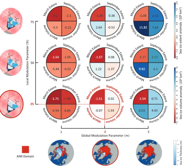
10.1029/2019EF001230Figure 2.The nine pie charts show the sea ice extent and volume anomalies in nine sensitivity simulations (2020–2040) compared to historical conditions (1850–2000) for March and September. The numbers inside the pie charts provide the anomalies in106km2for the sea ice extent and in103km3for the sea ice volume. Each pie chart corresponds to one combination of the Global Modulation Parameter (GMP; increasing from left to right) and the Local Modulation Parameter (LMP; increasing from bottom to top). The LMP and GMP choice defines the active AIM domain (red area in the GMP maps) and therefore the strength of the AIM in the simulations. The combination GMP=2m and LMP=25% (marked in red) is used for the 21st century AIM simulations. AIM = Arctic Ice Management.
temperatures: If they never fall below the freezing point, no ice can grow, irrespective of AIM. In contrast, the September sea ice extent and the sea ice volume at any time of the year are strongly sensitive to the two parameters, with larger values of the parameters leading to larger extent and volume. The influence exerted by the thickness threshold (the GMP) is stronger than the one by the local density/efficiency (LMP). The LMP has only a minor influence for GMP=1m, where the impact of AIM is generally weak because 1-m ice thickness is typically not enough to withstand the summer melt. The influence of the LMP grows with increasing GMP.
For the 21st century simulations discussed in the following we have chosen GMP=2m and LMP=25%.
This setting restores the summer sea ice extent, which largely determines the ice-albedo feedback, quite accurately to historical levels (Figure 2). Moreover, assuming that a single AIM device covers∼0.1km2, aver- aged over winter 2020–2040 this setting approximately corresponds to 106active devices (Figure 3, bottom), as envisaged by D17.
2.2. Arctic Sea Ice in the 21st Century with AIM
The unperturbed simulations without AIM coherently project a virtually ice-free Arctic ocean in late sum- mer after 2060 (Figure 3). The introduction of AIM in 2020 induces a strong and sudden perturbation of the sea ice state. At first a new quasi equilibrium close to historical conditions is reached within a few
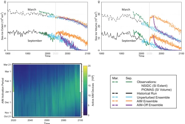
Figure 3.(top) Evolution of pan-Arctic sea ice extent (left) and volume (right) in March (upper curves) and September (lower curves). (bottom left) Daily number of active devices as a function of time of the year (vertical) and year (horizontal) in the AIM simulations (ensemble mean). NSIDC = National Snow and Ice Data Center; SI = sea ice;
PIOMAS = Pan-Arctic Ice Ocean Modeling and Assimilation System; AIM = Arctic Ice Management.
years. Compared to the unperturbed ensemble, the sea ice volume increases by∼40% in March and∼60% in September, and the September extent increases by∼40%, whereas the March extent is again hardly affected.
After the transition phase, however, the declining trend in sea ice volume is similar for both ensembles.
For the month of March (September), the declining sea ice volume trend is−163±2kmyear3(−121±3kmyear3) for the control ensemble mean and−182±3kmyear3(−144±2kmyear3) for the AIM ensemble mean (Table S1). Also, the September sea ice extent shows a clear declining trend due to the greenhouse gas-induced warming:
−8.3±0.3×10⁴ kmyear2 for the control ensemble mean and−6.2±0.2×10⁴ kmyear2 for the AIM ensemble mean (Table S1). Based on the sea ice extent trends of the two ensemble means, a virtually ice-free Arctic ocean (sea ice extent< 1×10⁶km2) occurs 66±6years later with AIM. While the exact delay depends on the parameter considered, overall the Arctic sea ice decline is delayed by roughly 60 years through AIM.
Our approach entails that the number of active AIM devices continuously changes in response to the spa- tial ice thickness distribution, both between years and within a freezing season (Figure 3, bottom left). In early 2020, immediately after the AIM activation, the number of active devices (20×106) is particularly large because the sea ice thickness is below the thickness threshold (GMP=2m) in most places. Until around 2060, the area of ice less than 2 m thick and hence the number of active devices tends to decrease monoton- ically from 10×106to≤ 5×10⁶devices over the course of each freezing season. After 2060 the seasonal maximum is shifted gradually toward the end of the freezing season because the greenhouse gas-induced warming impedes the thickness growth, so that the seasonal ice area growth becomes faster than the sea- sonal growth of the ice area with thickness≥2 m. Similarly, the seasonally averaged number of active devices grows toward the end of the century because the ice area with thickness≥2 m declines more rapidly than the total ice area.
If AIM would generate unanticipated detrimental effects of any kind, it would be important that the approach is reversible. To test this, we have branched off four additional simulations from the AIM ensem- ble in 2030 where AIM is turned off. The sea ice extent and volume return to the unperturbed trajectory within a transition period of less than 10 years (Figure 3, purple curves). This is consistent with earlier find- ings that there is no tipping point associated with Arctic sea ice and the ice-albedo feedback (Tietsche et al.,
Earth’s Future
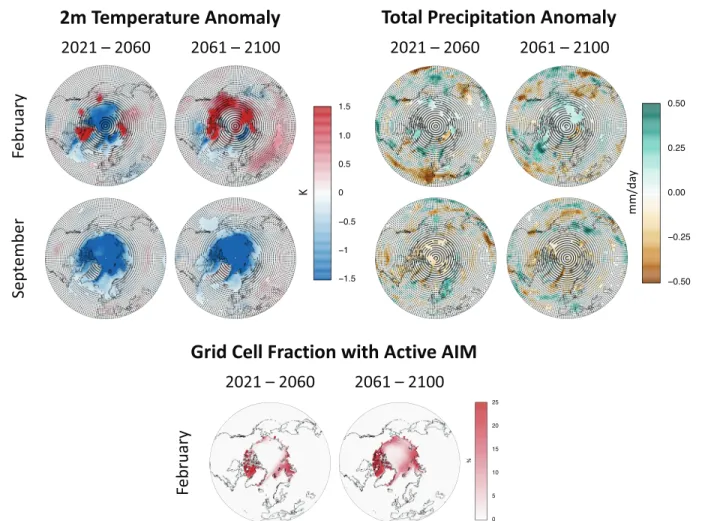
10.1029/2019EF001230Figure 4.(top left) Near-surface (2 m) temperature anomalies (AIM ensemble mean minus unperturbed ensemble mean) for the periods 2021–2060 and 2061–2100. (top right) As before but for the total precipitation anomaly. (bottom) Grid cell fraction with active AIM devices. Note that the 25% upper boundary is defined by the GMP. Stippling indicates local statistical nonsignificance of the anomaly at the 95% confidence level according to a two-tailedttest.
AIM = Arctic Ice Management; GMP = Global Modulation Parameter.
2011) and suggests that AIM is fully reversible. While this can be regarded as a beneficial property of AIM, it also implies that the array of devices would need to be maintained constantly to stay on a trajectory with delayed Arctic sea ice decline. The rapid loss of the response to geoengineering once it is discontinued seems to be common to geoengineering techniques trying to alter the Earth's albedo (McCusker et al., 2014).
2.3. The Climate Impact of AIM
The increased surface albedo associated with the additional sea ice results in significantly more reflected solar radiation in the Arctic during summer (∼5.0 W/m2at the top of the atmosphere in July north of the polar circle for 2021–2060;∼6.5 W/m2for 2061–2100; see also Figure S4). Averaged over the globe, the solar radiative forcing due to AIM amounts to∼0.25 W/m2in July (for 2021–2060 as well as 2061–2100) but only
∼0.02 W/m2for 2021–2060 and∼0.08 W/m2for 2061–2100 when averaged over the whole year. The latter corresponds to slightly more than half of the estimate by D17 and a quarter of the estimate by Hudson (2011) for a summer ice-free Arctic Ocean.
In the Arctic, AIM leads to a consistent late-summer cooling (Figure 4, top left; September). Averaged over the area north of the polar circle, September near-surface (2 m) temperatures are reduced by∼1.3 K during the first half of the simulations (2021–2060) and by∼1.4 K during the second half (2061–2100) compared to the unperturbed simulations. The Arctic winter response is more heterogeneous in both space and time (Figure 4, top left; March). In February, most areas of the Arctic Ocean are cooled by AIM during the first decades (average temperature anomaly over cooling regions is∼ −1.1K), whereas some peripheral seas including the Baffin Bay area and the Kara Sea are subject to additional near-surface warming (average temperature anomaly over warming regions is∼1 K); on average the Arctic is cooled by∼0.3 K. Toward
the end of the century the regions with AIM-induced warming expand further into the Arctic Ocean; the average Arctic cooling turns into a warming by∼0.5 K. This adds to the 10.7 K of Arctic February warming in 2061–2100 relative to historical conditions in the unperturbed simulations.
The Arctic temperature response (Figure 4, top left) is caused mainly by four mechanisms:
1. In winter, the AIM devices maintain a layer of liquid water approximately at the freezing point on the ice surface. This leads to strongly enhanced surface heat fluxes and warm temperature anomalies in areas with active devices. This explains the February warming that expands gradually from the peripheral regions to the central Arctic. Figure 4 shows a clear correspondence between regions with warm temperature anomalies (top left; February) and the active AIM regions (bottom).
2. Some marginal thin-ice regions of the Arctic ice cover experience winter cooling instead of warming despite active AIM devices, simply because these regions are ice-free in the unperturbed simulations.
These regions, including the northern Barents Sea, have gained ice through increased advection from AIM-affected upstream regions.
3. Regions with ice thicker than 2 m that were previously subject to AIM encounter weaker winter heat fluxes from the ocean to the cold atmosphere due to the increased ice thickness compared to the unperturbed simulations. Such thick-ice regions without AIM activity thus experience cold temperature anomalies.
This explains the February cooling in the central Arctic in 2021–2060.
4. In summer, the additional ice in the AIM ensemble has a direct cooling effect on the atmosphere and surface ocean by latent heat absorption associated with its melting, as well as an indirect cooling effect due to the increased surface albedo and accordingly reduced solar radiative heating. This explains the Arctic summer cooling.
While the impact of AIM on Arctic temperatures is substantial, lower-latitude regions are only weakly affected. The strongest influence outside the Arctic is exerted on the northern North Atlantic (Figure 4, top left). In particular, the Irminger Sea and the Labrador Sea are affected by enhanced ice export from the Arc- tic. The additional ice leads to a moderate cooling by up to∼1 K that prevails year-round throughout the century, but the Atlantic Meridional Overturning Circulation is not sensitive to these changes (Figure S5).
Outside the northern North Altlantic, the temperature response to AIM is weak and mostly not statistically significant. Some late-century anomalies, like the winter warming in central Eurasia and the summer cool- ing south of Alaska, appear to be locally significant (Figure 4, top left), but limited field significance for the middle and low latitudes as a whole suggests that these temperature anomalies might be spurious.
The annual-mean near-surface temperature response of the northern middle latitudes (30–60◦N) to AIM is close to 0 (∼ −0.04 K and∼ −0.02 K in the first and second half of the simulations), with minor seasonality.
This means that the middle-latitude warming obtained with the extreme-AIM experiment (Figure S2) can be prevented with a careful regulation of the interference. However, a significant cooling outside the Arctic (and northern North Atlantic) is still not accomplished. The annual global-mean near-surface warming of
∼1.9 and∼3.6 K in the first and second halves of the unperturbed simulations is reduced by only∼0.02 and
∼0.05 K, despite the intervention in the Arctic ice-albedo feedback.
Finally, a large-scale interference with the climate system can in principle also affect other relevant aspects of climate besides radiation and temperature. The most obvious additional impact of AIM in our simula- tions is an enhancement of the hydrological cycle and precipitation in regions with warming and moistening due to active devices in winter (Figure 4, top right; March). We also find a drying across the Arctic Ocean in summer (Figure 4, top right; September), albeit less significant than the associated cooling. The precipita- tion response beyond the Arctic is weak, and small regions with locally significant anomalies again appear not to withstand field significance considerations. In general, the large-scale circulation does not respond coherently to AIM in our simulations, despite the modified meridional near-surface temperature gradient.
We conclude that the impact of AIM on climate outside the Arctic (and the northern North Atlantic) is generally weak.
3. Discussion
This study involves a number of simplifying assumptions and approximations. The AIM implementation neglects peculiarities associated with ice formation at the surface instead of the bottom. Differences in the
Earth’s Future
10.1029/2019EF001230amount of salt rejected during the freezing and related to the flooding of the snow cover would have implica- tions for the physical properties of the resulting sea ice, including its surface reflectivity and its mechanical behavior. More generally, the use of a single climate model with necessarily simplified representations for all components of the physical climate system implies that our results are subject to uncertainty.
The difference between our estimate for the global annual-mean solar radiative forcing of AIM (0.08 W/m2 for 2061–2100) and the estimates by D17 (0.14 W/m2) and Hudson, (2011; 0.3 W/m2) can have various rea- sons. The amount of clouds prevailing over the Arctic in summer for instance modulates the impact of changes in surface albedo. However, the Arctic summer cloud cover in our simulations amounts to about 80%, which is in line with the assumptions and observations used in D17 and Hudson (2011). We also do not find a response of the summer cloud cover that would be strong enough to explain the difference (Figure S4). Other relevant factors include the assumed or simulated ice surface albedo and how it develops when melt ponds form (which is treated by a diagnostic melt pond scheme in our model) as well as the assumed or simulated sea ice area difference. In fact the latter might explain why D17 arrive at a higher estimate: They assume that the albedo change would occur over the entire area of the Arctic Ocean (107km2), whereas the ice extent anomalies in our simulations amount to roughly half of that area (depending on the year and time of the year; compare Figure 3 for September).
Another element of uncertainty arises from the way we regulate the strength of AIM: Our implementation implicitly assumes that the deployment and relocation of devices is accomplished so efficiently that the evolving areas with ice thinner than 2 m are equipped with devices during the whole winter. Our estimate of∼10×106for the number of required devices, corresponding to the number suggested by D17, should thus be regarded as a lower bound.
Our work does not consider the economic and technical feasibility of the construction, deployment, and maintenance of the enormous array of AIM devices that would be required. It also does not touch the politi- cal and societal dimension associated with such a planetary-scale intervention. Moreover, we do not attempt to provide precise estimates for the impacts of AIM on the climate system. This also holds for possible impacts on permafrost thaw and associated carbon emissions due to the summer cooling and winter warm- ing in Arctic land regions. Rather, our results constitute a first assessment of the efficiency and impacts of AIM from a climate physics perspective. We find evidence that AIM can in principle delay the Arctic sea ice decline by several decades. Yet the cooling of lower latitudes, anticipated as a consequence of the inter- vention in the ice-albedo feedback, fails to materialize. These results cast doubt on the potential of sea ice targeted geoengineering as a meaningful contribution to mitigate climate change.
4. Methods
4.1. The AWI Climate Model
We use the AWI-CM (Rackow et al., 2016; Sidorenko et al., 2015) which contributes to the Coupled Model Intercomparison Project Phase 6 (CMIP6; Eyring et al., 2016). For the atmospheric model component ECHAM6 (Stevens et al., 2013) we use the coarse-resolution version with ∼1.8◦ grid spacing. For the unstructured-mesh ocean and sea ice model component FESOM1.4 (Timmermann et al., 2009) we use the
“CORE2” mesh with a resolution of∼25 km in the Arctic and∼1.27×10⁵surface nodes globally. Details on the influence of the model resolution of the two model components can be found in Sein et al. (2018) and Rackow et al. (2019). The sea ice model (Danilov et al., 2015) includes an elastic-viscous-plastic rheology and a thermodynamical component based on Parkinson and Washington (1979), including a prognostic snow layer (Owens & Lemke, 1990). The heat, momentum, and mass fluxes at the interface between the ocean (including the sea ice) and the atmosphere are computed within the atmospheric model and exchanged 6-hourly via the OASIS3-MCT coupler. The surface fluxes play a central role in this study because the implementation of AIM in AWI-CM is based on the modification of the surface exchange processes.
4.2. AIM Implementation
Our implementation of AIM acts on the vertical fluxes of heat, mass, and momentum across the ocean/ice-atmosphere interface. When AIM is active, it is assumed that a fraction of the sea ice defined by the LMP is covered by a thin but persistent water layer (PWL). The PWL has the same temperature as the sea surface and is thus close to the freezing point in regions with sea ice. The PWL is continuously restored by the AIM devices as soon as the water freezes or evaporates. The lower boundary of the atmosphere thus corresponds to an increased fraction of open water because the PWL masks the sea ice underneath. The
latent and sensible heat fluxes, which represent the turbulent part of the surface heat budget, are calculated for a correspondingly altered open water fraction. Likewise, the surface thermal emissivity and the surface albedo are set to open water values for the PWL-covered part, even though the shortwave radiation plays a minor role during the Arctic winter. Since the PWL covers the sea ice and inhibits ice sublimation, only evaporation from the PWL is allowed in the AIM-affected part of the ice surface. Snow has a temperature of at most 0◦C, whereas the PWL is close to the freezing point of salty sea water at∼ −1.8◦C. Snow falling into the PWL is thus immediately added to the ice mass without latent heat changes, whereas snow falling into open water is assumed to melt and absorb latent heat.
Formulated as a weighted average of the original fluxes over open water (w) and ice (i), the total heat flux Hand the total mass fluxMthus depend on the sea ice concentrationAiand the LMP as follows:
H=(
1−LMP·Ai) (
QwS +QwL+QwLW+QwSW) +(
LMP·Ai) (
QiS+QiL+QiLW+QiSW) +(
1−Ai) (
Psnow·Lf) M=(
1−LMP·Ai)
Eevap+(
LMP·Ai)
Esubl+Psnow+Prain
whereAiis the sea ice concentration,QLWandQSWare the net longwave and shortwave radiation,Prainand Psnoware the liquid and solid precipitation,Lfis the latent heat of fusion of melting ice,QSis the sensible heat flux,QL is the latent heat flux, andEsublandEevapare the sublimation and evaporation fluxes. The momentum flux calculation remains unchanged.
This modified formulation is used from 21 October to 21 March (the Arctic freezing season) in grid cells north of the polar circle (∼66.5◦N) where the ice thickness is below the GMP. No GMP is applied in the extreme AIM simulation.
Except for the described modifications, the sea ice physics remain the same as in the standard FESOM model. The sea ice model does not include a grounding scheme (i.e., no seabed stress is considered), and the ice thickness is not limited by the ocean depth, which has implications for the realism of our extreme AIM experiment in particular in shallow ocean regions.
4.3. Experimental Setup
Our CMIP-type simulations are designed to test the response of the climate system to AIM in a progressively warming climate. After a 700-year spin-up simulation with constant CMIP6 preindustrial (1850) forcing, we performed a single simulation until 1999 with transient CMIP6 historical forcing. In 2000, small per- turbations were applied to the atmospheric model to generate a four-member ensemble of simulations that continued until 2014 with CMIP6 historical forcing. Since the new CMIP6 scenario forcings (O'Neill et al., 2016) were not yet available at the time, we used CMIP5 scenario forcing from 2015 onward, accepting a minor discontinuity in the forcing. RCP 8.5 corresponds to the “business-as-usual” scenario where no sub- stantial efforts are implemented to curb greenhouse gas emissions. The four unperturbed simulations were conducted until 2100.
In 2020 a total of 13 simulations was branched off from the unperturbed simulations:
• One simulation with extreme AIM, that is, with LMP=100% and no GMP applied, until 2100;
• Nine sensitivity simulations combining three GMP values (1, 2, and 3 m) with three LMP values (25%, 50%, and 75%) until 2040, one of which (GMP=2 m, LMP=25%) is extended to 2100; and
• Three additional simulations with GMP=2 m and LMP=25% until 2100, with each member of the resulting four-member ensemble initialized from one of the four-member unperturbed ensembles.
4.4. Simulated Versus Observed Historical Sea Ice State
A realistic simulated sea ice state is an important prerequisite for a meaningful quantitative assessment of AIM. The Arctic sea ice extent simulated for the period 1979–2017 is in overall agreement with observations in terms of mean value, trend, and interannual variability (Figure 3, top left), although the model seems to slightly underestimate the March sea ice extent and fails to simulate years with particularly low sea ice extent as they occurred in 2007 and 2012. The AWI-CM slightly underestimates the Arctic sea ice volume compared to PIOMAS (Schweiger et al., 2011) during the period 1979–2005. The more recent volume values are better represented. Nevertheless, the model captures the declining sea ice volume trend (Figure 3, top right). The spatial thickness distribution is also realistically simulated, with thicker ice north of Greenland and the Canadian Archipelago compared to the rest of the Arctic (Figure S6). The modeled sea ice thickness can be visually compared to sea ice thickness satellite retrievals and reanalysis products (Ricker et al., 2017;
Wang et al., 2016).
Earth’s Future
10.1029/2019EF001230Acronyms
AIM Arctic Ice Management
AMOC Atlantic Meridional Overtourning Circulation D17 Desch et al. (2017)
AWI-CM Alfred Wegener Institute Climate Model CMIP6 Coupled Model Intercomparison Project Phase 6 LMP Local Modulation Parameter
GMP Global Modulation Parameter NSIDC National Snow and Ice Data Center
PIOMAS Pan-Arctic Ice Ocean Modeling and Assimilation System PWL Persistent Water Layer
TOA Top of the Atmosphere
References
Altmetric Attention Score (2017). Arctic ice management. Retrieved from https://wiley.altmetric.com/details/14862679#score (Accessed:
2019–11–18).
Bellamy, R., Lezaun, J., & Palmer, J. (2017). Public perceptions of geoengineering research governance: An experimental deliberative approach.Global Environmental Change,45, 194–202. https://doi.org/10.1016/j.gloenvcha.2017.06.004
Blackstock, J. J., & Long, J. C. S. (2010). The politics of geoengineering.Science,327(5965), 527–527. https://doi.org/10.1126/science.
1183877
Comiso, J. C. (2011). Large decadal decline of the Arctic multiyear ice cover.Journal of Climate,25(4), 1176–1193. https://doi.org/10.1175/
JCLI-D-11-00113.1
Cornwall, W. (2015). Inside the Paris climate deal.Science,350(6267), 1451–1451. https://doi.org/10.1126/science.350.6267.1451 Cvijanovic, I., Caldeira, K., & MacMartin, D. G. (2015). Impacts of ocean albedo alteration on Arctic sea ice restoration and Northern
Hemisphere climate.Environmental Research Letters,10(4), 44020. https://doi.org/10.1088/1748-9326/10/4/044020
Danilov, S., Wang, Q., Timmermann, R., Iakovlev, N., Sidorenko, D., Kimmritz, M., et al. (2015). Finite-Element Sea Ice Model (FESIM), version 2.Geoscientific Model Development,8(6), 1747–1761. https://doi.org/10.5194/gmd-8-1747-2015
Desch, S. J., Smith, N., Groppi, C., Vargas, P., Jackson, R., Kalyaan, A., et al. (2017). Arctic ice management.Earth's Future,5, 107–127.
https://doi.org/10.1002/2016EF000410
Eyring, V., Bony, S., Meehl, G. A., Senior, C. A., Stevens, B., Stouffer, R. J., & Taylor, K. E. (2016). Overview of the Coupled Model Intercomparison Project Phase 6 (CMIP6): Experimental design and organization.Geoscientific Model Development,9(5), 1937–1958.
https://doi.org/10.5194/gmd-9-1937-2016
Field, L., Ivanova, D., Bhattacharyya, S., Mlaker, V., Sholtz, A., Decca, R., et al. (2018). Increasing Arctic sea ice albedo using localized reversible geoengineering.Earth's Future,6, 882–901. https://doi.org/10.1029/2018EF000820
Givens, J. E. (2018). Geoengineering in context.Nature Sustainability,1, 459–460. https://doi.org/10.1038/s41893-018-0140-y Hamilton, C. (2013). No, we should not just at least do the research.Nature News,496(7444), 139. https://doi.org/10.1038/496139a Hudson, S. R. (2011). Estimating the global radiative impact of the sea ice-albedo feedback in the Arctic.Journal of Geophysical Research,
116, D16102. https://doi.org/10.1029/2011JD015804
Intergovernmental Panel on Climate Change (2014). Long-term climate change: Projections, commitments and irreversibility pages 1029 to 1076.
Jahn, A. (2018). Reduced probability of ice-free summers for 1.5◦C compared to 2◦C warming.Nature Climate Change,8(5), 409–413.
https://doi.org/10.1038/s41558-018-0127-8
Kay, J. E., Holland, M. M., & Jahn, A. (2011). Inter-annual to multi-decadal Arctic sea ice extent trends in a warming world.Geophysical Research Letters,38, D16102. https://doi.org/10.1029/2011JD015804
Keith, D. (2001). Geoengineering.Nature,409, 420. https//doi.org/:10.1038/35053208
Lindsay, R., & Schweiger, A. (2015). Arctic sea ice thickness loss determined using subsurface, aircraft, and satellite observations.The Cryosphere,9(1), 269–283 https://doi.org/10.5194/tc-9-269-2015
Manabe, S., & Stouffer, R. J. (1980). Sensitivity of a global climate model to an increase of CO2concentration in the atmosphere.Journal of Geophysical Research,85(C10), 5529–5554. https://doi.org/10.1029/JC085iC10p05529
McCusker, K. E., Armour, K. C., Bitz, C. M., & Battisti, D. S. (2014). Rapid and extensive warming following cessation of solar radiation management.Environmental Research Letters,9(2), 24005. https://doi.org/10.1088/1748-9326/9/2/024005
Mengis, N., Martin, T., Keller, D. P., & Oschlies, A. (2016). Assessing climate impacts and risks of ocean albedo modification in the Arctic.
Journal of Geophysical Research: Oceans,121, 3044–3057. https://doi.org/10.1002/2015JC011433
Niederdrenk, A. L., & Notz, D. (2018). Arctic sea ice in a 1.5◦C warmer world.Geophysical Research Letters,45, 1963–1971 en. https://doi.
org/10.1002/2017GL076159
Notz, D., & Stroeve, J. (2016). Observed Arctic sea-ice loss directly follows anthropogenic CO2emission.Science,354, 747–750. https://doi.
org/10.1126/science.aag2345
Notz, D., & Stroeve, J. (2018). The trajectory towards a seasonally ice-free Arctic ocean.Current Climate Change Reports,4, 407–416. https://
doi.org/10.1007/s40641-018-0113-2
O'Neill, B. C., Tebaldi, C., van Vuuren, D. P., Eyring, V., Friedlingstein, P., Hurtt, G., et al. (2016). The Scenario Model Intercomparison Project (ScenarioMIP) for CMIP6.Geoscientific Model Development,9(9), 3461–3482. https://doi.org/10.5194/gmd-9-3461-2016 Owens, W. B., & Lemke, P. (1990). Sensitivity studies with a sea ice-mixed layer-pycnocline model in the Weddell Sea.Journal of Geophysical
Research,95(C6), 9527–9538. https://doi.org/10.1029/JC095iC06p09527
Parkinson, C. L., & Washington, W. M. (1979). A large-scale numerical model of sea ice.Journal of Geophysical Research,84(C1), 311–337.
https://doi.org/10.1029/JC084iC01p00311
Pithan, F., & Mauritsen, T. (2014). Arctic amplification dominated by temperature feedbacks in contemporary climate models.Nature Geoscience,7(3), 181–184. https://doi.org/10.1038/ngeo2071
Acknowledgments
The data in support of this publication have been deposited to the PANGAEA repository and are freely accessible (Zampieri, L. and Goessling, H.F.
(2019): Sea ice targeted geoengineering simulation with the AWI Climate Model. Alfred Wegener Institute, Helmholtz Centre for Polar and Marine Research, Bremerhaven, PANGAEA, https://doi.org/10.1594/
PANGAEA.906077). We are very grateful to the FESOM and AWI-CM development team at the Alfred Wegener Institute for Polar and Marine Research (AWI) and to Dirk Barbi and Nadine Wieters for their technical support. Furthermore, we are thankful to Thomas Jung, Mike Steele, and the Forum for Arctic Ocean Modeling and Observational Synthesis (FAMOS) community for the support and very helpful discussions. We also thank our colleagues at the Max Planck Institute for Meteorology for providing ECHAM6. We acknowledge the financial support of the Federal Ministry of Education and Research of Germany in the framework of the research group Seamless Sea Ice Prediction (SSIP; Grant 01LN1701A).
Finally, we acknowledge the NSIDC for making their sea ice extent data available (at https://nsidc.org/data/
G02135/477versions/3) as well as the Polar Science Center for the PIOMAS sea ice volume product (at http://psc.
apl.uw.edu/wordpress/wpcontent/
uploads/schweiger/icevolume/
PIOMAS.2sst.monthly.Current.v2.1.
txt).
Rackow, T., Goessling, H. F., Jung, T., Sidorenko, D., Semmler, T., Barbi, D., & Handorf, D. (2016). Towards multi-resolution global climate modeling with ECHAM6-FESOM. Part II: Climate variability.Climate Dynamics,50, 2369–2394. https://doi.org/10.1007/
s00382-016-3192-6
Rackow, T., Sein, D. V., Semmler, T., Danilov, S., Koldunov, N. V., Sidorenko, D., et al. (2019). Sensitivity of deep ocean biases to horizontal resolution in prototype CMIP6 simulations with AWI-CM1.0.Geoscientific Model Development,12, 2635–2656. https://doi.org/10.5194/
gmd-12-2635-2019.
Ricker, R., Hendricks, S., Kaleschke, L., Tian-Kunze, X., King, J., & Haas, C. (2017). A weekly Arctic sea-ice thickness data record from merged CryoSat-2 and SMOS satellite data.The Cryosphere,11(4), 1607–1623. https://doi.org/10.5194/tc-11-1607-2017
Rogelj, J., den Elzen, M., Höhne, N., Fransen, T., Fekete, H., Winkler, H., et al. (2016). Paris Agreement climate proposals need a boost to keep warming well below 2◦C.Nature,534(7609), 631–639. https://doi.org/10.1038/nature18307
Schweiger, A., Lindsay, R., Zhang, J., Steele, M., Stern, H., & Kwok, R. (2011). Uncertainty in modeled Arctic sea ice volume.Journal of Geophysical Research,116, C00D06. https://doi.org/10.1029/2011JC007084
Sein, D. V., Koldunov, N. V., Danilov, S., Sidorenko, D., Wekerle, C., Cabos, W., et al. (2018). The relative influence of atmospheric and oceanic model resolution on the circulation of the North Atlantic Ocean in a coupled climate model.Journal of Advances in Modeling Earth Systems,10, 2026–2041. https://doi.org/10.1029/2018MS001327
Seitz, R. (2011). Bright water: Hydrosols, water conservation and climate change.Climatic Change,105(3-4), 365–381. https://doi.org/10.
1007/s10584-010-9965-8
Serreze, M. C., Barrett, A. P., Slater, A. G., Steele, M., Zhang, J., & Trenberth, K. E. (2007). The large-scale energy budget of the Arctic.
Journal of Geophysical Research,112, D11122. https://doi.org/10.1029/2006JD008230
Sidorenko, D., Rackow, T., Jung, T., Semmler, T., Barbi, D., Danilov, S., et al. (2015). Towards multi-resolution global climate model- ing with ECHAM6-FESOM. Part I: Model formulation and mean climate.Climate Dynamics,44(3), 757–780. https://doi.org/10.1007/
s00382-014-2290-6
Stevens, B., Giorgetta, M., Esch, M., Mauritsen, T., Crueger, T., Rast, S., et al. (2013). Atmospheric component of the MPI-M Earth System Model: ECHAM6.Journal of Advances in Modeling Earth Systems,5, 146–172. https://doi.org/10.1002/jame.20015
Stroeve, J. C., Kattsov, V., Barrett, A., Serreze, M., Pavlova, T., Holland, M., & Meier, W. N. (2012). Trends in Arctic sea ice extent from CMIP5, CMIP3 and observations.Geophysical Research Letters,39, L16502. https://doi.org/10.1029/2012GL052676
Talberg, A., Thomas, S., Christoff, P., & Karoly, D. (2018). How geoengineering scenarios frame assumptions and create expectations.
Sustainability Science,13(4), 1093–1104. https://doi.org/10.1007/s11625-018-0527-8
Tietsche, S., Notz, D., Jungclaus, J. H., & Marotzke, J. (2011). Recovery mechanisms of Arctic summer sea ice.Geophysical Research Letters, 38, L02707. https://doi.org/10.1029/2010GL045698
Timmermann, R., Danilov, S., Schroeter, J., Boening, C., Sidorenko, D., & Rollenhagen, K. (2009). Ocean circulation and sea ice distribution in a finite element global sea ice-ocean model.Ocean Modelling,27(3), 114–129. https://doi.org/10.1016/j.ocemod.2008.10.009 Trodahl, H. J., Wilkinson, S. O. F., McGuinness, M. J., & Haskell, T. G. (2001). Thermal conductivity of sea ice; dependence on temperature
and depth.Geophysical Research Letters,28, 1279–1282. https://doi.org/10.1029/2000GL012088
United Nations (2015). Paris Agreement. https://unfccc.int/sites/default/files/english_paris_agreement.pdf (Accessed: 2019–11–18).
Wallace, J. M., & Hobbs, P. V. (2006).Atmospheric science: An introductory survey. Amsterdam: Elsevier Academic Press.
Wang, X., Key, J., Kwok, R., & Zhang, J. (2016). Comparison of Arctic sea ice thickness from satellites, aircraft, and PIOMAS data.Remote Sensing,8(9), 713. https://doi.org/10.3390/rs8090713