Oxygen fluxes beneath Arctic land‑fast ice and pack ice: towards estimates of ice productivity

(1)

https://doi.org/10.1007/s00300-018-2350-1 ORIGINAL PAPER

Oxygen fluxes beneath Arctic land‑fast ice and pack ice:

towards estimates of ice productivity

Karl M. Attard^1,2,3 · Dorte H. Søgaard³ · Judith Piontek⁴ · Benjamin A. Lange^5,6 · Christian Katlein⁵ · Heidi L. Sørensen¹ · Daniel F. McGinnis^7,8 · Lorenzo Rovelli¹ · Søren Rysgaard^3,9,10 · Frank Wenzhöfer^5,11 · Ronnie N. Glud^1,12

Received: 10 January 2018 / Revised: 25 April 2018 / Accepted: 4 June 2018

Abstract

Sea-ice ecosystems are among the most extensive of Earth’s habitats; yet its autotrophic and heterotrophic activities remain poorly constrained. We employed the in situ aquatic eddy-covariance (AEC) O₂ flux method and laboratory incubation techniques (H¹⁴CO₃⁻, [³H] thymidine and [³H] leucine) to assess productivity in Arctic sea-ice using different methods, in conditions ranging from land-fast ice during winter, to pack ice within the central Arctic Ocean during summer. Labora- tory tracer measurements resolved rates of bacterial C demand of 0.003–0.166 mmol C m⁻² day⁻¹ and primary productivity rates of 0.008–0.125 mmol C m⁻² day⁻¹ for the different ice floes. Pack ice in the central Arctic Ocean was overall net autotrophic (0.002–0.063 mmol C m⁻² day⁻¹), whereas winter land-fast ice was net heterotrophic (− 0.155 mmol C m⁻² day⁻¹). AEC measurements resolved an uptake of O₂ by the bottom-ice environment, from ~ − 2 mmol O₂ m⁻² day⁻¹ under winter land-fast ice to~ − 6 mmol O₂ m⁻² day⁻¹ under summer pack ice. Flux of O₂-deplete meltwater and changes in water flow velocity masked potential biological-mediated activity. AEC estimates of primary productivity were only possible at one study location. Here, productivity rates of 1.3 ± 0.9 mmol O₂ m⁻² day⁻¹, much larger than concurrent laboratory tracer estimates (0.03 mmol C m⁻² day⁻¹), indicate that ice algal production and its importance within the marine Arctic could be underestimated using traditional approaches. Given careful flux interpretation and with further development, the AEC technique represents a promising new tool for assessing oxygen dynamics and sea-ice productivity in ice-covered regions.

Keywords Sea-ice · Primary production · Bacterial production · Carbon cycling · Eddy-covariance

* Karl M. Attard

karl.attard@biology.sdu.dk

1 Department of Biology, University of Southern Denmark, 5230 Odense, Denmark

2 Tvärminne Zoological Station, University of Helsinki, J.A. Palménin tie 260, 10900 Hanko, Finland

3 Greenland Climate Research Centre, Greenland Institute of Natural Resources, 3900 Nuuk, Greenland

4 GEOMAR, Helmholtz Centre for Ocean Research Kiel, Kiel, Germany

5 Alfred Wegener Institute, Helmholtz Centre for Polar and Marine Research, Bremerhaven, Germany

6 University of Hamburg, Centre for Natural History (CeNak), Zoological Museum, Martin-Luther-King Platz 3, 20146 Hamburg, Germany

7 Aquatic Physics Group, Department F.-A. Forel

for Environmental and Aquatic Sciences (DEFSE), Section

of Earth and Environmental Sciences, Faculty of Sciences, University of Geneva, Uni Carl Vogt, 66 Boulevard Carl-Vogt, 1211 Geneva, Switzerland

8 Leibniz-Institute of Freshwater Ecology and Inland Fisheries (IGB), Mueggelseedamm 310, 12587 Berlin, Germany

9 Clayton H. Riddell Faculty of Environment Earth and Resources, University of Manitoba, Winnipeg, MB R3T 2N2, Canada

10 Arctic Research Centre, Department of Bioscience, Aarhus University, 8000 Aarhus, Denmark

11 HFG-MPG, Joint Research Group for Deep Sea Ecology and Technology, Max Planck Institute for Marine Microbiology, Bremen, Germany

12 Department of Ocean and Environmental Sciences, Tokyo University of Marine Science and Technology, Tokyo 108-8477, Japan

(2)

Introduction

Sea‑ice ecosystems

Sea-ice annually covers ~ 25 million km² of Earth’s surface (Parkinson and DiGirolamo 2016). In the central Arc- tic Ocean, sea-ice extent ranges from ~ 15 million km² in March to < 4 million km² in September, and additionally covers numerous fjords, sounds, and embayments at lower latitudes (Arrigo 2014; NSIDC 2017). Sea-ice provides a complex and rigid floating structure in an otherwise open ocean, and supports diverse lifeforms that range from microorganisms living within the ice matrix to fish, birds, and mammals seeking sanctuary on or beneath the ice (Thomas 2017). The bottom-ice layer typically is the most biologically-productive sea-ice habitat. Microscopic algae that accumulate within this region due to favorable growth conditions constitute a primary food source for grazers located within the immediate vicinity of the ice pack (Kohlbach et al. 2016). In aggregated forms, algae can sink rapidly to depths of several kilometers and sus- tain opportunistic deep-sea benthic communities (Boetius et al. 2013). Living in close association with the ice algae are heterotrophic microbes that play a significant role in the sea-ice microbial ecosystem. Through diverse meta- bolic functions and interactions, communities of protists and bacteria effect key biogeochemical transformations of carbon and nutrients in Arctic surface waters (Bowman 2015).

Organisms inhabiting the sea-ice are at the mercy of a highly unpredictable ecosystem where thermodynamics, divergence, and deformation processes continuously alter habitat characteristics (Thomas 2017). During ice formation, dissolved constituents of seawater such as the salts and gases are expelled from the ice. With sustained cool- ing from the atmosphere, ice grows in thickness. The accu- mulated brines percolate through the ice matrix and under the action of gravity are forced downward, forming vertical interlinked channels through the ice and draining to the underlying waters. Sea-ice is therefore largely depleted of dissolved salts and gases, but the brine channels form a mosaic of microsites within the ice pack which typically are at or close to saturation with respect to dissolved gases (Glud et al. 2002; Zhou et al. 2014; Galley et al.

2015). Colder ice temperatures favor low brine volume, high brine salinity, and low permeability of the ice matrix (Cox and Weeks 1983). During the ice thaw, or under thick snow cover, ice porosity increases, and meltwater dilutes the existing brines and exchanges fluid with underlying waters (Hunke et al. 2011). Ice temperature, brine volume, and light availability alter the sea-ice O₂ pool through stimulating microbial respiration and primary production.

In warmer months and under light-limiting conditions (due to e.g., snow cover), the sea-ice O₂ pool may be further depleted through enhanced microbial respiration, potentially permitting anaerobic respiration pathways such as denitrification and anammox that influence nutrient availability for primary producers (Rysgaard and Glud 2004;

Rysgaard et al. 2008). Sympagic primary productivity rates and the distribution of photosynthetic organisms are further influenced by surface ice conditions such as snow thickness, melt-pond cover, and ice topography (Katlein et al. 2014, 2015).

Constraining autotrophic and heterotrophic activity in sea‑ice

While many of the mechanisms described above are well- known, measurements of autotrophic and heterotrophic activity rates, two key processes occurring within sea-ice, are relatively scarce within the literature. This is especially the case for measurements performed under in situ conditions whereby environmental conditions within the ice pack remain unaltered. Previous studies have documented that sea-ice productivity is dynamic and is driven by complex interactions between variables such as current strength and sunlight availability (McMinn et al. 2000). Sea-ice presents a challenge for productivity studies in that the ice pack is a solid, often uneven surface with a patchy distribution of biotic communities (Rysgaard et al. 2001; Glud et al. 2014;

Katlein et al. 2014). Laboratory incubation techniques (H¹⁴CO₃⁻ and [³H] thymidine) are the standard and widely accepted approach to assess rates of biological processes in sea-ice. However, incubation techniques are highly invasive and invoke considerable assumptions with scaling, core col- lection, sectioning, melting, and incubation of the meltwater in the laboratory (Miller et al. 2015). The heterogeneous nature of sea-ice makes tracers homogenization a challenge.

Methods utilizing O₂ in combination with inert gases (e.g., O₂:Ar) (Zhou et al. 2014) represent a promising new tool for investigating sea-ice productivity, but similarly require extraction of ice cores from the environment for laboratory analysis. In situ techniques such as pulse amplitude modu- lation (PAM) fluorometry and oxygen microprofiling at the ice–water interface are less invasive, but integrate over micro-scale regions of the under-ice habitat, and replication is difficult (McMinn et al. 2000; Kuhl et al. 2001; Rysgaard et al. 2001; Glud et al. 2002). It is therefore necessary to consider other non-invasive, complementary methods that are capable of integrating heterogeneous under-ice communities, such as sparsely-distributed ice algal encrustations and aggregates (Miller et al. 2015).

In recent years, sea-ice productivity has been quantified from direct, non-invasive biogeochemical O₂ flux measurements at the ice–water interface using an aquatic

(3)

eddy-covariance (AEC) approach (Long et al. 2012), a method originally designed for benthic applications (Berg et al. 2003). The AEC method infers areal-averaged fluxes of O₂ at the ice–water interface, typically in mmol O₂ m⁻² day⁻¹, by quantifying the turbulent transport of O₂ from within the under-ice boundary layer at some distance (~ 0.5 m) beneath the ice. Advantages of this method include its non-invasive nature, as well as its ability to integrate over patchy and heterogeneous biotic communities and surfaces (Rheuban and Berg 2013). While the AEC method clearly holds great potential for autotrophic and heterotrophic activity studies in sea-ice, the O₂ fluxes at the ice–water interface, from which the productivity measurements are derived, are influenced not only by biotic processes of photosynthetic production and respiration, but also by thermodynamic processes of ice freezing and melting (Glud et al. 2002, 2014;

Long et al. 2012). To our knowledge there exist just three applications of the AEC O₂ flux method to sea-ice: flux measurements beneath land-fast ice in a sub-Arctic fjord in Greenland (Long et al. 2012), pack ice in the Fram Strait (Glud et al. 2014), and a sea-ice pool study by Else et al.

(2015).

In this study, we investigate sea-ice productivity using AEC and traditional laboratory incubation approaches in different high-Arctic settings, representing a wide range of ice types and environmental conditions. The data are used to evaluate sea-ice productivity and its drivers as measured using the AEC technique, and how these values compare to laboratory incubation approaches.

Materials and methods

Study locations

This study incorporates data collected during two separate research expeditions to the high Arctic in 2012. The first expedition took place in March at the Daneborg field station (74º18.57′N, 20º18.27′W) located in Young Sound, North-east Greenland (Fig. 1) (Rysgaard and Glud 2007).

Sea-ice at this location is typical of fjord ice in the Arctic, often covered by large amounts of snow. Sampling here was performed at a single location on land-fast ice (ICE- 1, hereafter referred to as ‘DNB’) located ~ 2 km away

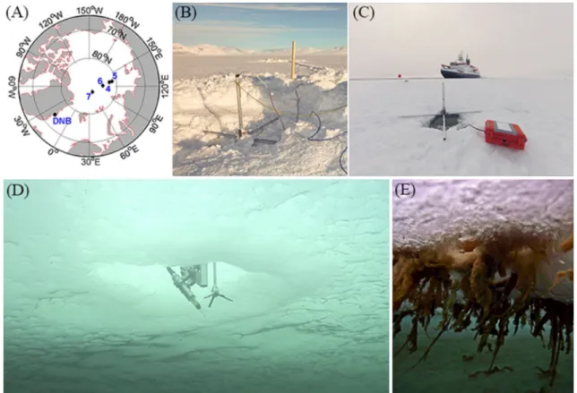
Fig. 1 Geographical location of the five measurement sites in North- east Greenland (station DNB) and the central Arctic Ocean (stations Ice 4 to Ice 7; a), b a top-side view of an AEC instrument deployed at station DNB in Greenland, c a top-side view of an AEC instrument deployed in the central Arctic Ocean, d an AEC instrument viewed

from below the ice using the ROV, and e filamentous strands formed by the centric diatom Melosira arctica attached to the underside of the ice in the central Arctic Ocean Photo by M. Fernández-Méndez taken nearby station Ice 7

(4)

from the Daneborg field station (Rysgaard et al. 2013). A second expedition took place later that year to the central Arctic Ocean (RV Polarstern IceArc Expedition (ARK27- 3), 2 August to 8 October; Fig. 1) (Boetius 2013). Suc- cessful measurements during this second campaign were performed on pack ice at four separate ice stations, located between 82 and 87°N, and cover a range of environmental conditions, ranging from first-year sea-ice (FYI) with high melt-pond cover at the ice edge, to thicker multi-year ice (MYI) nearby the geographic North Pole (Fig. 1).

Environmental conditions above the ice

Weather stations located at the Daneborg field station and on the research vessel measured air temperature (°C), wind velocity (m s⁻¹) and direction, and incident solar radiation (W m⁻²) during both sampling campaigns at 10 min intervals. Incident solar radiation was converted to incoming photosynthetically active radiation (PAR, in µmol photons m⁻² s⁻¹) following calibration on-site to a Li-Cor Quantum 2-pi sensor (R² > 0.95; Li-Cor Biosciences).

Ice temperature and salinity

Measurements of ice temperature and salinity were performed on ice core samples, extracted using a Mark II Coring System (9 cm inner diameter, Kovacs Enterprises, Roseburg, Oregon, USA). Ice temperature was measured at 5–10 cm intervals using a calibrated digital penetration thermometer (Testo Limited, Hampshire, United King- dom). Ice salinity was calculated from conductivity measurements performed on melted sections of the ice cores.

The cores were cut into 10 cm sections using a stainless- steel saw, and the individual sections were kept thawing in the dark and at a temperature of 3 ± 1 °C. Approximately 48 h later, once the samples had thawed completely, conductivity measurements were performed using conductivity sensors (Thermo Orion-Star with an Orion 013610MD conductivity cell, ThermoFisher Scientific, Massachu- settes, USA; WTW 3300i, Wissenschaftlich-Technische Werkstätten GmbH, Weilheim, Germany). Ice salinity was subsequently calculated from conductivity according to Grasshoff et al. (2007).

Sea-ice brine volume for intact ice samples was calculated from measured ice salinity, bulk density, and temperature according to Leppäranta and Manninen (1988) for temperatures > − 2 °C, and according to Cox and Weeks (1983) for temperatures < − 2 °C. Ice porosity (ϕ), also known as ‘void fraction’, was calculated from ice density (σ) as 𝜙=1− 𝜎_bulk∕𝜎_ice , where a value of 917 kg m⁻³ was used for pure ice (Yen et al. 1991).

Sea‑ice primary productivity and bacterial C demand measurements

Depth-integrated measurements of potential sea-ice primary productivity and bacterial C demand were performed following standard procedures as described by Søgaard et al.

(2010). The advantages and disadvantages of these methods are well-known and have been given careful consid- eration within the literature (Miller et al. 2015; Campbell et al. 2017). Potential sea-ice primary productivity (PP_i) was quantified by performing H¹⁴CO₃^– incubations on melted ice sections under different irradiance levels (260, 140, 43, 0 µmol photons m⁻² s⁻¹). Individual incubations lasted 5 h and were maintained at a temperature of 3 ± 1 °C. Illumina- tion was provided from a 150 W fiber optic tungsten-halo- gen bulb that emits light with a spectral distribution similar to that of natural sunlight. Primary productivity rates (in µg C kg⁻¹ ice h⁻¹) for each sea-ice section were dark-corrected, plotted against the irradiance levels, and fitted with the photosynthesis-irradiance (P–E) function described by Platt et al. (1980) using a least-squares approach. Derived P–E relationships for the different ice depths were scaled to hourly measurements of above-ice incident irradiance, accounting for light attenuation due to overlying snow and ice as described by Søgaard et al. (2010). Depth-integrated rates of daily PP_i (in mmol C m⁻² ice day⁻¹) were calculated as the sum of the daily PP_i at the different ice depths.

Sea-ice bacterial C demand rates (BP_i) were similarly determined using incubation techniques for different sections of melted sea-ice. In Greenland, measurements were performed directly on melted sea-ice samples, whereas in the central Arctic, ice core sections were melted in a known volume of artificial seawater. In all cases, a slow melting process was applied (Mikkelsen and Witkowski 2010).

BP_i was determined from incorporation of either tritium- labeled thymidine ([³H] thymidine, Greenland campaign) or [³H] leucine (central Arctic Ocean). In Greenland, tripli- cate samples of 10 mL meltwater were extracted from each melted ice section, and were incubated for 6 h in darkness at 3 ± 1 °C with 10 nM of labeled [³H] thymidine (specific activity 10.1 Ci mmol⁻¹, New England Nuclear), along with trichloroacetic acid (TCA)—killed controls to measure potential abiotic adsorption. At the end of the incubation period, 1 mL of 50% cold TCA was added to all the samples for fixation. The samples were filtered and counted using a liquid scintillation analyzer (TricCarb 2800, PerkinElmer).

BP_i measurements for the Arctic Ocean campaign were quantified from the uptake of [³H] leucine (specific activity 107.7 Ci mmol⁻¹, Perkin Elmer). Subsamples of 20 mL were incubated with [³H] leucine at a final concentration of 20 nmol L⁻¹ for 13–17 h. Incubation was terminated by add- ing TCA at a final concentration of 5%. Cells were then collected by filtration onto 0.2 µm-polycarbonate filters. Each

(5)

filter was rinsed three times with 1 mL of a 5% TCA solu- tion. Filters were dried and the incorporation of [³H] leucine into the TCA-insoluble fraction was measured by liquid scintillation counting, performed on-board the research vessel after addition of scintillation cocktail (Ultima Gold AB, Perkin Elmer). Results were corrected for dilution with artificial seawater and for abiotic absorption estimated from TCA-killed controls. For both [³H] thymidine and [³H]

leucine treatments, bacterial C production was calculated using the conversion factors presented in Smith and Clem- ent (1990). Carbon production rates were divided by growth efficiency (0.5) (Rivkin and Legendre 2001) to compute bacterial C demand (in µg C kg⁻¹ ice h⁻¹), and the values for the individual ice layers were subsequently summed to derive depth-integrated rates (in mmol C m⁻² day⁻¹). For comparison of PP_i and BP_i with other rate measurements, we assume a C:O₂ of 1.0.

Environmental conditions beneath the ice

A conductivity-temperature-depth (CTD) sonde (SBE 19 plus V2, Seabird) was deployed at 0.5–1.0 m depth beneath the ice to monitor the under-ice environmental conditions.

The CTD logged water temperature, salinity, depth, PAR (QCP-2000, Biospherical Instruments), and O₂ concentration in the water by means of a calibrated optode (4340, Aanderaa) at 30 s intervals.

During the central Arctic Ocean expedition, light transmittance through sea-ice was measured using a RAMSES- ACC hyperspectral radiometer (TriOS Datentechnik, Rast- ede, Germany) carried on-board a V8-Sii (Ocean Modules, Åtvidaberg, Sweden) remotely operated vehicle (ROV). The vehicle, operated directly from the ice through a manually cut access hole, was piloted beneath the ice along horizontal transects to resolve the spatial variability in light transmittance due to e.g., melt ponds and ridges (Nicolaus and Katlein 2013). Successful ROV dives were performed at all ice stations except for Ice 4, where the ROV could not be operated due to an electronic failure. Measurements with a distance of more than 2 m to the ice were discarded during processing. Details about the deployment method and data processing can be found in the report by Katlein et al.

(2012).

Microgradients of O₂ at the ice–water interface Vertical microprofiles of O₂ at the ice–water interface were obtained in situ using an underwater microprofiling unit (Boetius and Wenzhoefer 2009), that was mounted onto an ice profiler system with an articulated arm. The ice profiler, similar to the system of McMinn et al. (2000), consisted of a horizontal arm carrying an elevator system and an underwater electronic cylinder housing. The sensor module

consisted of two Clark-type O₂ microelectrodes, one resistiv- ity sensor, and one temperature sensor for high-resolution measurements, together with an oxygen optode (Aanderaa 4330) and an underwater PAR sensor (Li-Cor UWQ8312).

The instrument was deployed through a 50 × 50 cm ice hole.

The articulated arm positioned the sensors 2 m away from the hole, to minimize light interference. The raw O₂ microsensor output was calibrated to the dissolved O₂ concentration in µmol O₂ L⁻¹ in water and ice using a two-point calibration. The first point was obtained from the in situ O₂ concentration in the water as measured by the optode, and the second point was obtained in the laboratory as the zero sensor reading. A thin metal rod attached to the electronic cylinder protruded 5 cm longer than the sensors, and was used as a reference for initial sensor array positioning directly below the sea-ice interface. The microsensors were then programmed to sample and record data while moving at 100 µm vertical steps toward the ice. We limit our interpretation of the microprofiles to the ice–water interface (i.e., water-side measurements) only, since the microsensor signal output may be compromised when in contact with solid ice crystals (Glud et al. 2002).

Eddy‑covariance O₂ fluxes

Fluxes of O₂ between sea-ice and the underlying water were quantified using our standard AEC system that is similar to the original design used by Berg and Huettel (2008) for measuring benthic fluxes of O₂. This instrument consists of a 6 MHz acoustic Doppler velocimeter (ADV; Nortek, Norway) and two Clark-type O₂ microsensors that relay an amplified signal to the velocimeter via submersible ampli- fiers (Revsbech 1989; McGinnis et al. 2011). The microsensors were individually tested for their quality prior to deployment, and had a 90% response time of ≤ 0.3 s and a stirring sensitivity of ≤ 1% (Gundersen et al. 1998). Sensor stirring sensitivity effects on the O₂ fluxes were estimated using the formulations provided by Holtappels et al. (2015) to be a minor bias in the data (< 7%). The O₂ sensors were affixed to the stem of the ADV using a polyoxymethylene mounting and the sensors were positioned at an angle of 60°

relative to the velocimeter, with the ~ 20 µm microsensor tips located 0.5 cm away from the instrument’s 2.65 cm³ cylindrical-shaped measurement volume (McGinnis et al.

2011). The AEC instrumentation was deployed vertically through a hole in the ice, attached to a sturdy 2 m-long alu- minum pipe section with the measurement volume located at a depth of ~ 0.5 m below the ice (Fig. 1) (Long et al.

2012). Online readings were used to align the instrument coordinates within the main flow direction. Flow velocity and O₂ microsensor output were logged in continuous sampling mode at 64 Hz, with measurements periodically being interrupted for data download or sensor replacement.

(6)

Processing of the raw AEC data followed established protocols for bin-averaging the 64 Hz data to 8 Hz, despik- ing, coordinate rotation, and quality checking individual flux intervals for anomalous data such as jumps in O₂ concentration (Lorrai et al. 2010; Long et al. 2012; Berg et al. 2013;

Attard et al. 2015; Else et al. 2015). Sensor calibration, flux extraction, and time-shifting of the O₂ data for maximum numerical flux were performed using the Sulfide Oxygen Heat Flux Eddy Analysis (SOHFEA) software (www.dfmcg innis .com/SOHFE A) (McGinnis et al. 2014). The raw O₂ microsensor signal was calibrated using linear regression against in situ O₂ concentrations obtained from an O₂ optode that was located on the nearby (~ 20 m distant) CTD sonde.

Impacts of averaging timescales and sensor response on the O₂ flux were investigated by expressing the vertical flux w^′O^′₂ as the integrated value of the cospectrum of w^′O^′₂ in the frequency (f) domain (termed ‘cumulative cospectra’) (Berg et al. 2003; Lorrai et al. 2010), as

The cumulative cospectra were used to evaluate the frequency of the flux-contributing turbulent eddies, the optimal averaging time scales to use for scalar flux extraction, as well as any flux loss from spectral attenuation due to sensor response time and separation distances (Lorke et al. 2013;

Donis et al. 2015). Following this analysis, fluxes of O₂ in mmol O₂ m⁻² day⁻¹ were extracted using linearly detrended 15 min ensemble average intervals that were subsequently bin-averaged to 1 h intervals. Positive O₂ fluxes indicate a release of O₂ by the bottom-ice environment and negative fluxes indicate O₂ uptake.

Constraining the O₂ flux due to basal ice melt

The O₂ flux due to bottom-ice formation or melt was estimated from heat flux measurements performed at the ice–water interface as described by Long et al. (2012). At the DNB site, heat flux measurements were performed by direct covariance, using a fast-response temperature sensor (FP07, ISW Wassermesstechnik, Germany; accuracy ± 0.02 °C, resolution 0.002 °C, response time 10 ms) that was interfaced with the ADV. Data processing followed the same procedure described above for extracting the O₂ fluxes from the raw data streams, and the fluxes of heat (H_f, in W m⁻²) were calculated according to the equation

where T is water temperature, 𝜌_sw and C_p the density and specific heat capacity of seawater, respectively. Because direct covariance fluxes of heat were only available during the first campaign, the under-ice ocean heat flux for the

(1) w^�O^�₂=

∞

∫

0

Co_w�O^�

2(f)df .

(2) H_f =w^�T^�𝜌_swC_p,

second research campaign was estimated from bulk measurements of water temperature elevation above freezing (𝛿_T) and friction velocity (

u_∗)

as described by McPhee et al.

(1999, 2016):

where 𝛿_T=T−T_f , with T (°C) the water temperature beneath the ice and T_f (°C) is the freezing point of saltwater calculated from salinity S and pressure p (dbar) as

C_H is the bulk heat transfer coefficient (0.0085) (Sirevaag 2009; McPhee et al. 2016) and c_w is the specific heat capacity of seawater (3980 J kg⁻¹ °C⁻¹). Measurements of S , T , and p were performed by the CTD probe at a depth of 0.5–1.0 m below the ice. The CTD sensors are accurate to within ± 0.0005 S m⁻¹ for conductivity and to ± 0.005 °C for T . The u_∗ was computed from the acoustic velocimeter data streams as the square root of the Reynolds stress magnitude (Berg et al. 2007). First, the streamwise (u) , traverse (v) and vertical (w) velocity components were decomposed into mean and deviatory velocities as u= ̄u+u^� , v= ̄v+v^� , and w= ̄w+w^� . The u_∗ was then derived as

The u_∗ was computed as a function of the ensemble averaging interval where a time window of 15 min was deemed to be suitable for deriving u_∗ (McPhee 2008).

Assuming that all of the excess under-ice heat went into melting ice, the computed H_f was used to estimate rates of ice melt (h, in mm day⁻¹) as

where ΔH_f is the specific heat of fusion of ice (333.55 kJ kg⁻¹), and 𝜌_i is the bulk density of ice (measured; bottom 10 cm = 805–959 kg m⁻³). The melted ice volume was multiplied by 0.89 to compute meltwater volume released per unit area of sea-ice per day (L m⁻² day⁻¹).

The O₂ flux rate due to basal thermodynamics (TO_2f) was then calculated by assuming that the released meltwater was anoxic and at a temperature of 0 °C, consistent with the assumption of O₂- and salt-free parent ice (Glud et al. 2002).

Every liter of anoxic meltwater released would thus appear within the measured O₂ fluxes as an “uptake” of 456.6 µmol O₂ by the ice, representing the theoretical upper limit of O₂ exchange at the ice–water interface due to basal ice formation or melt (Long et al. 2012). Since this analysis considers only basal ice melt, this approach provides a minimum estimate of the impact of meltwater on the measured eddy fluxes.

(3) H_f = 𝜌_swc_pc_Hu_∗𝛿_T,

Tf = −0.057S+( (4)

1.710523×10⁻³) S^1.5

−(

2.154996×10⁻⁴) S²−(

7.53×10⁻⁴) p

(5) u_∗=(

u^�w^�²+v^�w^�²)1∕4

.

(6) h= H_f

ΔH_f𝜌_i

(7)

Results

Ice stations

The land-fast ice station (DNB) had 115 cm-thick sea-ice covered by 70 cm of snow. Freeboard was negative, resulting in an 8 cm slush snow layer at the snow-ice interface.

Average air temperature for this campaign was − 25 ± 10 °C.

The sampled stations between 82 and 85°N in the central Arctic (Ice 4, Ice 5 and Ice 6) were characterized by a heavily degraded first-year ice pack in advanced stages of melt, with sea-ice thickness frequently < 1.0 m, ice coverage down to 50%, and up to 50% melt-pond cover (Table 1).

Average air temperature at these sites ranged from 0.3 ± 0.6 to − 3.2 ± 0.5 °C. In contrast, station Ice 7 consisted of a multi-year ice floe that was less degraded in comparison, and had a relatively homogenous ice thickness of ~ 1.8 m.

Station Ice 7 was sampled in the second half of September, when air temperature was cooler and freezing conditions in melt ponds and leads were observed. In all cases, snow depth was ≤ 6 cm (Table 1).

The ice-associated phototrophic biomass at stations Ice 4 to Ice 7 consisted largely of diatoms within the ice matrix and melt ponds, and more conspicuously as aggregates in two distinct forms: (1) spherical aggregations composed mainly of pennate diatoms such as Nitzschia sp.

and Navicula sp. and (2) filamentous strands of the centric diatom Melosira arctica attached to the underside of the ice (Fernández-Méndez et al. 2014). Under-ice aggregate abundance, quantified using ROV image surveys conducted within the vicinity (40–350 m distant) of our instrumented areas of each ice floe, ranged from 0.3 aggregates m⁻² at Ice

5 to 3.8 aggregates m⁻² at Ice 7, with an estimated average biomass of 0.1–6.5 mg C m⁻² (Katlein et al. 2014).

Ice temperature, salinity and porosity

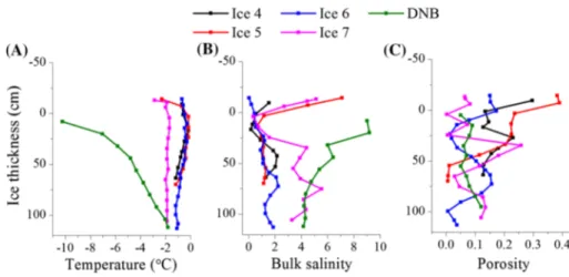
Ice temperature ranged from − 10 to − 0.1 °C, with the coolest temperatures measured within the upper ice layers at DNB, and the warmest temperatures measured in the mid- dle ice sections at Ice 5 (Fig. 2). Temperature within the bottom-ice layer was less variable and ranged from − 1.1 to

− 1.9 °C. Ice salinity was between 0.1 and 9.2. Brine volume calculated from ice T, S, and ρ indicated high porosity at Ice 4, Ice 5, and Ice 6 above 0.1 and reaching as high as 0.4 at Ice 5. Station Ice 7 was somewhat less variable with porosity values between 0.01 and 0.12 (Fig. 2).

Oxygen microprofiles

Under-ice microprofiling was attempted at stations Ice 3–6.

Deploying the instrument correctly with the sensor tip positioned nearby the ice–water interface is an inherently difficult procedure due to the uneven underside of the ice floe, and the need to position the fragile sensors nearby the solid boundary without having an accurate visual reference aid.

Successful measurements were made at stations Ice 3–5, and even here only single O₂ microprofiles were collected, due to sensor damage incurred following contact of the sensor tip and/or penetration into the solid ice. Despite the challenges posed by this method, the available microprofiles for stations Ice 3–5 showed a consistent picture of steep O₂ gradients at the ice–water interface and highly O₂-depleted conditions within the ice (Fig. 3).

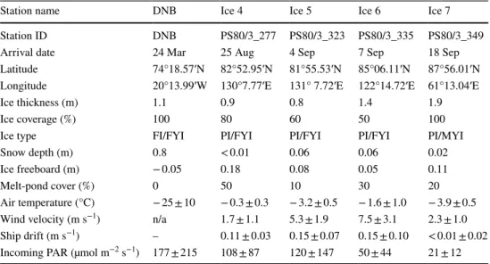
Table 1 Location and characteristics of the sea- ice stations investigated in Daneborg (DNB), North-east Greenland, and the central Arctic Ocean (stations Ice 4–7)

Above-ice environmental parameters are reported as mean ± SD over the ~ 2 day duration of each ice station. Ice type is classified as land-fast ice (FI) or pack ice (PI), first-year ice (FYI) or multi-year ice (MYI)

Station name DNB Ice 4 Ice 5 Ice 6 Ice 7

Station ID DNB PS80/3_277 PS80/3_323 PS80/3_335 PS80/3_349

Arrival date 24 Mar 25 Aug 4 Sep 7 Sep 18 Sep

Latitude 74°18.57′N 82°52.95′N 81°55.53′N 85°06.11′N 87°56.01′N

Longitude 20°13.99′W 130°7.77′E 131° 7.72′E 122°14.72′E 61°13.04′E

Ice thickness (m) 1.1 0.9 0.8 1.4 1.9

Ice coverage (%) 100 80 60 50 100

Ice type FI/FYI PI/FYI PI/FYI PI/FYI PI/MYI

Snow depth (m) 0.8 < 0.01 0.06 0.06 0.02

Ice freeboard (m) − 0.05 0.18 0.08 0.05 0.11

Melt-pond cover (%) 0 50 10 30 20

Air temperature (°C) − 25 ± 10 − 0.3 ± 0.3 − 3.2 ± 0.5 − 1.6 ± 1.0 − 3.9 ± 0.5 Wind velocity (m s⁻¹) n/a 1.7 ± 1.1 5.3 ± 1.9 7.5 ± 3.1 2.3 ± 1.0 Ship drift (m s⁻¹) – 0.11 ± 0.03 0.15 ± 0.07 0.15 ± 0.10 < 0.01 ± 0.02 Incoming PAR (µmol m⁻² s⁻¹) 177 ± 215 108 ± 87 120 ± 147 50 ± 44 21 ± 12

(8)

Light environment

Daily average incoming PAR was highest at DNB (177 ± 215 µmol m⁻² s⁻¹) and at Ice 4 and Ice 5 (~ 100 µmol m⁻² s⁻¹), decreasing to 50 ± 44 µmol m⁻² s⁻¹ at Ice 6 and 21 ± 12 µmol m⁻² s⁻¹ at Ice 7 (Table 1).

PAR transmittance, expressed as a % of incoming PAR,

was highest at Ice 4 (13%) and lowest at DNB (0.001%) (Table 2). Under-ice ROV measurements of light transmittance, available for Ice 5, Ice 6 and Ice 7, documented values that were highly variable on meter spatial scales (Fig. 4).

The highest range in transmittance values was measured at Ice 6 (from < 0.1 to 37.8%; mean ± SD = 4.2% ± 5.3 (n = 2326), median = 1.7%, mode = 1.3%), followed by Ice 5 (from < 0.1 to 21.8%; mean ± SD = 2.9% ± 2.3 (n = 2177), median = 2.5%, mode = 2.2%), and Ice 7 (from 0.2 to 18.4%; mean ± SD = 3.5% ± 2.9 (n = 553), median = 2.5%, mode = 1.2%).

Eddy‑covariance O₂ fluxes

High-quality O₂ fluxes were extracted from 81 to 96% of the collected AEC data. The DNB dataset consists of 62 h of continuous under-ice O₂ flux measurements whereas the central Arctic Ocean data consist of shorter 20–41 h datasets with a total of ~ 110 h of flux measurements divided between stations Ice 4–7. Well-developed turbulent conditions were evident at all five measurement locations, with the weighted spectra (i.e., the power spectral density multiplied by the wavenumber) of the vertical velocity variance showing a distinct peak in the area-preserving spectrum, as well as a fall-off to the − 2/3 slope in the log–log representation of the spectrum (McPhee 2008). Cumulative cospectra, computed for periods with high and low flow velocity, indicated a dom- inance of flux-contributing turbulent eddies within the frequency range of 0.0015 to 1 Hz. Flux convergence occurred between 0.0015 Hz (~ 660 s) and 0.001 Hz (1000 s), indicating that the selected averaging time scale of 900 s was optimal for flux extraction under the conditions we encoun- tered (Lorke et al. 2013). Temporal misalignment between velocity and O₂ concentration data streams that occurred due to sensor response time and sensor separation distances gave small errors in the flux estimates (< 10%), and this was corrected by shifting the O₂ data in time relative to the w data to compute the maximum numerical flux for w^′O^′

2 (McGinnis

Fig. 2 Bulk ice measurements of temperature (a), salinity (b), porosity (c) at the five measurement sites

Fig. 3 The under-ice microprofiler (a) that was used to measure O₂ concentration at the ice–water interface at three separate ice stations in the central Arctic Ocean (photo taken using the ROV). Steep O₂ gradients were present at the ice–water interface at all three measurement sites (b). The sensor signal is likely to be impacted by contact with the solid ice

(9)

et al. 2008). A time shift of 0.2–0.8 s was applied for this correction, which is in good agreement with the response time of the O₂ a sensors we used (Donis et al. 2015). Further evidence of well-developed turbulence and high-quality flux data was deduced from analysis of the cumulative instantaneous flux w^′O^′₂ , where linear trends indicate a stable flux signal (Fig. 5) (Berg et al. 2003; Long et al. 2012).

Average AEC O₂ fluxes were directed towards the ice (negative values) at all five stations, indicating an uptake of O₂ by the ice environment. Mean (± SD) fluxes ranged from

− 2.3 ± 8.0 mmol O₂ m⁻² day⁻¹ at DNB to − 6.2 ± 3.7 mmol O₂ m⁻² day⁻¹ at Ice 5 (Table 3). The flow velocity magnitude was the predominant driver of the O₂ fluxes at four of the five sites, with higher flow velocities resulting in higher O₂ uptake rates by the ice (Figs. 5, 6). The flow velocity, which in turn showed broad agreement in dynamics with the wind velocity, explained up to 92% of the hourly variations in the O₂ fluxes (Fig. 6).

Eddy‑covariance estimates of sea‑ice primary productivity

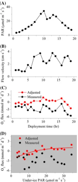
A tight coupling between the measured AEC O₂ fluxes and PAR availability, as one would expect due to photosynthetic production, was not immediately apparent at any of the investigated ice stations. Instead, the AEC fluxes at stations Ice 4–7 were significantly correlated to the water flow velocity, which masked any potential primary production effects. We excluded the flow velocity effects from the eddy fluxes by subtracting the relationship between the eddy fluxes and the flow velocity magnitude we established for each dataset (Fig. 6). Following this adjustment, patterns consistent with photosynthetic production were only evident at Ice 4, which is the study site where we observed the highest transmitted PAR values (Fig. 7, Table 2). Inter- estingly, the adjusted O₂ fluxes followed PAR dynamics. A modified photosynthesis-irradiance (P–E) curve fitted to the data (R² = 0.40) suggested that light saturation (E_k value)

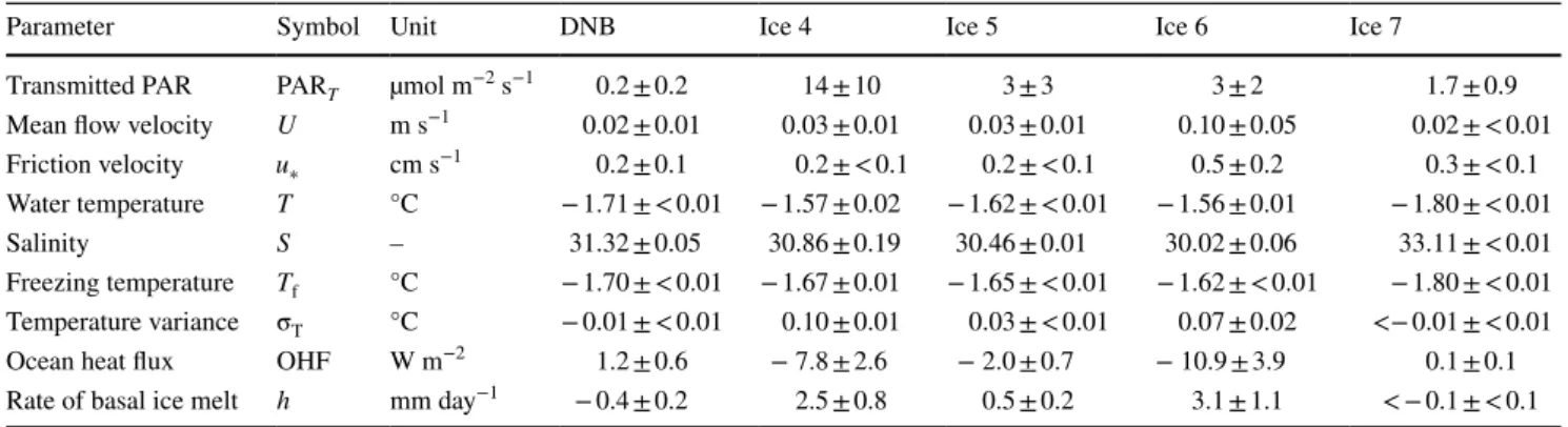
Table 2 Under-ice environmental parameters and fluxes (mean ± SD) for the five investigated locations

Negative fluxes indicate a flux directed towards the ice. Flow velocity is measured by the velocimeter 0.5 m beneath the ice

Parameter Symbol Unit DNB Ice 4 Ice 5 Ice 6 Ice 7

Transmitted PAR PART µmol m⁻² s⁻¹ 0.2 ± 0.2 14 ± 10 3 ± 3 3 ± 2 1.7 ± 0.9

Mean flow velocity U m s⁻¹ 0.02 ± 0.01 0.03 ± 0.01 0.03 ± 0.01 0.10 ± 0.05 0.02 ± < 0.01 Friction velocity u_∗ cm s⁻¹ 0.2 ± 0.1 0.2 ± < 0.1 0.2 ± < 0.1 0.5 ± 0.2 0.3 ± < 0.1 Water temperature T °C − 1.71 ± < 0.01 − 1.57 ± 0.02 − 1.62 ± < 0.01 − 1.56 ± 0.01 − 1.80 ± < 0.01

Salinity S – 31.32 ± 0.05 30.86 ± 0.19 30.46 ± 0.01 30.02 ± 0.06 33.11 ± < 0.01

Freezing temperature T_f °C − 1.70 ± < 0.01 − 1.67 ± 0.01 − 1.65 ± < 0.01 − 1.62 ± < 0.01 − 1.80 ± < 0.01 Temperature variance σ_T °C − 0.01 ± < 0.01 0.10 ± 0.01 0.03 ± < 0.01 0.07 ± 0.02 <− 0.01 ± < 0.01

Ocean heat flux OHF W m⁻² 1.2 ± 0.6 − 7.8 ± 2.6 − 2.0 ± 0.7 − 10.9 ± 3.9 0.1 ± 0.1

Rate of basal ice melt h mm day⁻¹ − 0.4 ± 0.2 2.5 ± 0.8 0.5 ± 0.2 3.1 ± 1.1 < − 0.1 ± < 0.1

Fig. 4 PAR transmittance values as measured by the ROV at Ice 6 indicate a heterogeneous light environment due to the heavily ponded and deformed ice pack (a). Frequency distribution analyses (b) sug-

gest clustering of transmittance values at around 8–10% for this par- ticular dataset, depending on the method used to describe the average

(10)

occurred above 16 µmol PAR m⁻² s⁻¹, and no photo inhi- bition was observed up to maximum transmitted light levels of 36 µmol PAR m⁻² s⁻¹ (Fig. 7). By assuming that (a) gross primary productivity under the lowest irradiance level of 3 µmol PAR m⁻² s⁻¹ was zero and that (b) any change in O₂ release under higher irradiance relative to that zero point was caused by photosynthetic production, we can estimate the daily primary productivity rate at Ice 4 as the mean (± SD) of all of the daytime hourly fluxes, which is 1.3 ± 0.9 mmol O₂ m⁻² day⁻¹ (n = 17).

Laboratory measurements of autotrophic and heterotrophic activity

Sea-ice bacterial C demand rates ranged from 0.003 to 0.166 mmol C m⁻² day⁻¹, with the highest value being measured at DNB on land-fast ice during winter. Ice primary productivity rates ranged from 0.008 to 0.125 mmol C m⁻² day⁻¹. Ice primary productivity values for the central Arctic Ocean were obtained from Fernán- dez-Méndez et al. (2015). The laboratory measurements indicate an overall net heterotrophic ice habitat at DNB (− 0.155 mmol C m⁻² day⁻¹), whereas the ice at the four

Fig. 5 A ~ 24 h time series of environmental conditions above and below the ice [PAR (a), temperature (b), flow velocity (c)] and under- ice eddy-covariance O₂ fluxes (d) in the central Arctic Ocean at station Ice 6. Linear cumulative instantaneous O₂ fluxes (e) indicate a good flux signal. Error bars are SD (n = 4). Negative fluxes indicate oxygen uptake by the ice

Table 3 Eddy-covariance fluxes beneath the ice and estimated rates of biological activity within the ice

*Values for the central Arctic Ocean (Ice 4–7) are from Fernández-Méndez et al. (2015)

Parameter Symbol Unit DNB Ice 4 Ice 5 Ice 6 Ice 7

Eddy-covariance O₂ flux AEC mmol O₂ m⁻² day⁻¹ − 2.3 ± 8.0 − 3.5 ± 3.0 − 6.2 ± 3.7 − 5.8 ± 3.5 − 3.2 ± 3.6

Bacterial C demand BP mmol C m⁻² day⁻¹ 0.166 0.006 0.006 0.003 0.062

Primary production* PP mmol C m⁻² day⁻¹ 0.011 0.033 0.008 0.017 0.125

Auto-heterotroph balance BP-PP mmol C m⁻² day⁻¹ − 0.155 0.027 0.002 0.014 0.063

Thermodynamic-induced O₂

flux (basal) TO_2f mmol O₂ m⁻² day⁻¹ 0.2 ± 0.1 − 1.1 ± 0.4 − 0.2 ± 0.1 − 1.4 ± 0.5 0.0 ± 0.0

Fig. 6 Relationship between the under-ice flow velocity magnitude and the eddy-covariance O₂ fluxes for the complete datasets at the four measurement sites in the central Arctic (Ice 4–7, panels a–d) and for the site in Greenland (Daneborg, panel e). The solid red line is a linear regression fitted to the data.

Broken lines are the 95% con- fidence bands. Negative fluxes indicate uptake by the ice

(11)

stations in the central Arctic Ocean was net autotrophic (up to 0.07 mmol C m⁻² day⁻¹; Table 3).

Heat fluxes, ice melt rate and physical‑induced O₂ exchange

Average H_f ranged from − 10.9 ± 3.9 W m⁻² at Ice 6 to 1.2 ± 0.6 W m⁻² at DNB (Table 2). The direction of the flux is indicated by its preceding sign, where negative values indicate an uptake of heat by the ice. The ocean was a source of heat to the ice at stations Ice 4–6, with temperature variance (𝜎_T) highest at Ice 4 (0.10 ± 0.01 °C) and lowest at Ice 5 (0.03 ± < 0.01 °C; Table 2). Assuming that all the excess

heat went into melting ice, the rate of ice melt at Ice 6 was

~ 3 mm day⁻¹ and for station Ice 5 it was ~ 0.5 mm day⁻¹. In contrast to this, supercooled waters were found at Ice 7 and DNB, with average 𝜎_T of up to − 0.01 ± < 0.010 °C and thus potential for ice growth. Estimated heat fluxes were low (− 0.1 to − 1.2 W m⁻²) as were rates of ice growth (negative melt equals growth; < 0.5 mm day⁻¹). Estimates of the O₂ exchange rate due to bottom-ice growth or decay were computed from the H_f to investigate the potential imprint of thermodynamic (physical) processes on the O₂ flux at the ice–water interface as measured by AEC (Long et al. 2012).

The O₂ flux due to basal ice melt was estimated to be a minor component, accounting for a maximum of 30% of the difference between the AEC flux magnitude and laboratory measures of biotic activity (Table 3).

Discussion

AEC O₂ fluxes: biological versus physical contributions

This study employs AEC and laboratory incubation techniques to assess autotrophic and heterotrophic productivity in sea-ice across a broad range of ice types and environmental conditions, from land-fast ice during winter to first-year and multi-year ice floes in the central Arctic Ocean during summer. This dataset constitutes an opportunity to investigate the rates and drivers of O₂ fluxes at the sea ice–water interface as measured using AEC, and the extent to which these measurements represent biological versus physical processes.

To date, applications of the AEC method in the Arc- tic have mostly focused on seafloor ecosystems. Here, the method constitutes a strong tool for quantifying primary productivity, respiration, and the net ecosystem metabolism rates non-invasively across complex and hard benthic surfaces that characterize much of the Arctic coastal zone (Glud et al. 2010; Attard et al. 2014, 2016). Sea-ice represents a challenge for metabolism studies similar to hard benthic surfaces, in that the underside of the ice pack is a solid, often uneven surface with a patchy distribution of biotic communities (Rysgaard et al. 2001; Katlein et al. 2014;

Lange et al. 2016). The AEC approach could therefore be a highly beneficial tool and would complement other methods in sympagic productivity investigations. While overcoming the inherent challenges of incubation approaches, as well as other approaches that rely upon extraction of ice samples for analysis, the O₂ fluxes as measured by AEC beneath the ice are complicated by ice thermodynamics and meltwater discharge, whereby biological O₂ production or consumption may be masked by a much larger physical-induced flux under conditions of freezing or melting (Glud et al. 2014;

Fig. 7 A 17 h time series at Ice 4 of a under-ice PAR availability, b water flow velocity, and c eddy-covariance O₂ fluxes before (black) and after (red) subtracting the effects of flow velocity. Eddy fluxes versus light availability for the same data before and after adjustment (d). The fitted modified P–E relationship (R² = 0.40) had a maximum rate of primary productivity (P_m) of 3.7 mmol O₂ m⁻² day⁻¹ and a light saturation (E_k) value of 16 µmol PAR m⁻² s⁻¹

(12)

Else et al. 2015). In this study, the AEC fluxes consistently suggested O₂ uptake rates by the ice environment at the 5 different study locations ranging from − 2.3 mmol O₂ m⁻² day⁻¹ at DNB to − 6.2 mmol O₂ m⁻² day⁻¹ at Ice 5 (Table 3).

These rates are 1–3 orders of magnitude higher than those of bacterial C demand performed on the same ice floes (range from 0.003 to 0.166 mmol C m⁻² day⁻¹; Table 3), the lat- ter at the lower end of bacterial C demand rate estimates for sea-ice in Greenland and in the Fram Strait (range from 0.06 to 3.37 mmol C m⁻² day⁻¹) (Søgaard et al. 2010, 2013;

Kaartokallio et al. 2013; Glud et al. 2014). Similar incon- sistencies between the laboratory and in situ techniques are identified for the resolved autotrophic-heterotrophic balance of the ice floes: whereas AEC measurements suggest an uptake of O₂ by the ice environment, laboratory measures suggest net autotrophy at stations Ice 4–7 (Table 3). Differ- ences between the two methodologies employed are clear and may account for variations in the resolved rates; however, the magnitude and direction of the AEC O₂ fluxes are consistent with a release of O₂-deplete meltwater. Under-ice microprofile measurements documented steep O₂ gradients at the ice–water interface (Fig. 3), with the gradient direction being in agreement with the O₂ flux directed towards the ice as measured using AEC, and confirms other microsensor measurements performed in melting sea-ice (Kuhl et al.

2001; Glud et al. 2002). Meltwater O₂ fluxes have the same sign (direction) as heterotrophic processes in the ice, so the AEC fluxes measured during dark would represent the sum of these two processes. During daytime, photosynthetic O₂ production would offset the O₂ uptake rate, but the primary productivity rate in the investigated ice floes is likely to be smaller than the sum of meltwater- and respiration-driven O₂ flux, resulting in an overall “uptake” of O₂ by the bottom-ice environment over 24 h as measured using AEC. Glud et al.

(2014) made similar observations for melting pack ice in the Fram Strait. Despite a significant ice-associated primary production and light-dependent O₂ exchange dynamics at this site, under-ice fluxes as measured by AEC suggested a net uptake of O₂ by the ice environment of 8 mmol O₂ m⁻² day⁻¹ due to a large (~ 25 L m⁻² day⁻¹) meltwater flux. Reli- able estimates of heterotrophic activity in sea-ice quantified using AEC would thus require accurate measurements of meltwater-driven O₂ flux.

Within the marginal ice zone of the central Arctic Ocean (~ 82–84°N), drifting of ice floes into warmer water result in large ice–water H_f of > 100 W m⁻² and rapid bottom ablation rates of several cm day⁻¹ (McPhee et al.

1987; Perovich et al. 1989; Peterson et al. 2017). The effect of such a large release of O₂-depleted meltwater could bias the O₂ fluxes as measured by AEC by > 10 mmol O₂ m⁻²−day⁻¹ (Glud et al. 2014). However, during our study, maximum temperature variance ( 𝜎_T ) was 0.10 °C and H_f

were in all cases < 11 W m⁻², with comparatively low bottom-ice ablation rates of ≤ 3 mm day⁻¹ resulting in maximum physical-induced O₂ exchange rates < 1.5 mmol O₂ m⁻² day⁻¹ (Tables 2, 3). This analysis suggests that ice melt from below was not a major contributor to the AEC O₂ fluxes during our measurement period (Table 3), and that other processes not included in this analysis must be important. Absorption of solar radiation by the ice, ice cracks, meltwater in ponds, and surface water in open leads can have a big impact on the heat and mass balance of sea-ice (Eicken et al. 2002; Hudson et al. 2013). This is likely to be an important process not accounted for in our calculations. Heat fluxes associated with drainage, advec- tion, and convection of warm meltwater may exceed the net solar shortwave flux, with wind stress helping to sus- tain fluid flow into ice neighboring a pond or lead (Eicken et al. 2002). The meltwater would accumulate on the surface as melt ponds, or drain through the ice matrix and fill the pore spaces, ultimately accumulating beneath the ice and exchanging with underlying waters. Ice temperatures around 0 °C were evident at several of the ice stations in the central Arctic Ocean, particularly within the upper layers of the ice, and melt-pond cover was between 10 and 50%. Ice porosity was frequently above 0.20 and as high as 0.40 at Ice 5 (Fig. 2). These values are much higher than the critical brine volume fraction of ~ 5% (porosity of

~ 0.05) that typically marks the transition from imperme- able to permeable sea-ice (Golden et al. 1998), indicating that these ice layers are potentially a large reservoir for meltwater, and are susceptible to extensive advective and convective meltwater exchange. Aside from the effects on the measured AEC fluxes, the O₂-depleted meltwater within the ice could be of considerable ecological signifi- cance for microbes and fauna living within the ice matrix (Kiko et al. 2017; Sørensen et al. 2017).

It is conceivable that accumulation and draining of meltwater may not be at steady-state, and that meltwater accumulation and release at the ice–water interface may not necessarily represent the surface ice melt rate during the period of assessment. Future studies would benefit from better constraining the meltwater flux. This could be achieved by performing AEC measurements of conductivity (salt) fluxes alongside temperature and O₂ (Else et al. 2015). More important, however, would be to target periods when the ice is at or near steady-state. It is evident from our measurements, and from those by Glud et al. (2014) and Else et al. (2015), that variations in the O₂ fluxes due to physical effects can by far exceed biotic O₂ production and consumption rates when performed under dynamic ice growth or melt, which complicates flux interpretation.