Institut für Numerische und Angewandte Mathematik

(1)

Institut für Numerische und Angewandte Mathematik

System Headways in Line Planning

M. Friedrich, M. Hartl, A. Schiewe, A. Schöbel

Nr. 11

Preprint-Serie des

Instituts für Numerische und Angewandte Mathematik Lotzestr. 16-18

D - 37083 Göttingen

(2)

System Headways in Line Planning ^∗

Markus Friedrich

¹

, Maximilian Hartl

¹

, Alexander Schiewe

²

, and Anita Sch¨ obel

²

1 University of Stuttgart, Pfaffenwaldring 7. 70569 Stuttgart, Germany, {markus.friedrich,maximilian.hartl}@isv.uni-stuttgart.de

2 University of Goettingen, Lotzestraße 16-18, 37083 G¨ottingen, Germany, {a.schiewe,schoebel}@math.uni-goettingen.de

Abstract

Line Planning is an important stage in public transport planning. This stage determines which lines should be operated with which frequencies.

Several integer programming models provide solutions for the line planing problem. However, when solving real-world instances, integer optimization often falls short since it neglects objectives that are hard to measure, e.g., memorability of the system. Adaptions to known line planning models are hence necessary.

We analyze one such adaption, namely that the frequencies of all lines should be multiples of a fixedsystem headway. This is common in practice and improves memorability and practicality of the designed line plan. We model the requirement of such a common system headway as an integer program and compare line plans with and without this new requirement theoretically by investigating worst case bounds, as well as experimentally on artificial and close to real-world instances.

Keywords: Public Transport Planning, Line Planning, Integer Op- timization

1 Introduction

Line planning in public transport is a well researched problem. Its goal is to choose the number and the shape of the lines to be operated and to determine their frequencies, i.e., how often services should be offered along every line within the planning period T. The lines together with their frequencies are called a line concept. Existing models optimize the costs, e.g., [5], [11], the number of direct travelers, e.g., [7],[4], or the approximated passengers’ traveling times, e.g., [17], [20] of the line concept. Overviews on different models can be found in [18] and [14].

∗This work was partially funded by DFG research unit FOR 2083.

(3)

Recent developments include different planning stages into the line planning problems, i.e., they consider integrated planning in public transport. Examples are to integrate the timetabling step [3], the demand [21] or treating several planning stages in an integrated way [19, 13]. Other work examine the effect of time dependent demand [2] or the differences of route choice and assignment [10].

Nevertheless, solutions to the line planning problem often fall short in important criteria that are not easily measurable in integer optimization problems.

One important criterion is the memorability of the resulting timetable. Ideally, public transport passengers need to memorize only one specific minute and a headway for a particular stop, e.g., minute 01 every 10 minutes. To achieve such properties, transport planners use specific concepts when designing line plans.

One common concept is a system or pulse headway describing a minimum headway, which must be achieved by all lines, see [23] and [22]. The application of a system headway leads not only to regular departure times but also to regular connections when passengers have to transfer.

More precisely, let a line concept consisting of a set of lines L and their frequenciesfl for all l ∈ L be given. If there exists a natural number i 6= 1 which is a common divisor of all frequenciesfl we say that the line concept has asystem headway.

In this paper, we want to model the concept of a system headway mathe- matically. In particular, we show how the requirement for a system headway can be added to existing integer optimization models, and we derive properties for general line planning models and for a cost-based formulation.

2 Modeling system headways

Before we introduce our adaptions to the integer programming models, we define formally what the line planning problem is. Let a public transport network PTN=(V, E) be given, with nodesV as stations and undirected edgesEbetween them. Aline l is a path in the PTN. In this paper we assume that a line pool L is given. It contains a (large) set of potential lines from which we want to choose the ones to establish. Aline concept (L, f) assigns a frequencyfl∈N0

to every line l in the given line pool L. (Lines which are not chosen from the pool receive a frequency of zero).

There exist many different models for line planning. The frequenciesflfor all l∈ Lare the variables to be determined in all line planning models. Sometimes, additional variablesx∈X ⊆Rⁿ are also present which might for example be used for modeling the paths of the passengers.

(4)

Thegeneral line planning model can hence be written as (P) min obj(f, x)

s.t. g(f, x) ≤ b

fl ∈ N0 for alll∈ L

x ∈ X,

where g : L ×X → R^m is a linear function containing m constraints and b∈R^m. Common choices for the linear objective functionobj:L ×X →Rare to minimize the costs or the traveling time of the passengers, or to maximize the number of direct travelers. The constraints are written in the general form g(f, x)≤b, but as noted in [18] most line planning models contain constraints of the type

X

l∈L:

e∈l

fl≥f_e^min ∀e∈E, (LEF)

and of the type

X

l∈L:e∈l

f_l≤f_e^max ∀e∈E (UEF)

for given lower and upper edge frequency bounds f_e^min ≤f_e^max for every edge e∈E. The constraints (LEF) are calledlower edge frequency constraints and are used to ensure that all passengers can be transported while theupper edge frequency constraints (UEF) are needed due to the limited capacity of tracks, or due to noise restrictions. They also bound the costs of the line concept.

Allowing to set f_e^min = 0 and f_e^max = ∞ we can without loss of generality assume that constraints of type (LEF) and (UEF) always are present in the general line planning model.

Typically, cost-oriented models minimize the costs of a line concept and contain (LEF) while passenger-oriented models optimize the traveling time or the number of transfers passengers have. To prevent the model to establish all lines with high frequencies, constraints of type (UEF) may be used or a budget constraint (BUD) (see Section 5).

The main definition for this work is the following.

Definition 1. Asystem headway (also calledsystem frequency) is defined as a common divisor of all frequenciesf_l, l∈ L, i.e.,i∈Nis a system headway for (L, f) if and only ifi≥2 andi|f_lfor alll∈ L.

In the following we look for line concepts which have a system headway. Note that we only consider system headways greater than one, as choosingi= 1 as a system headway poses no restriction on the model and is therefore considered as having no system headway at all.

Including the system headway requirement into the general line planning model (P) is possible with only small adaptions. Let us first consider a given

(5)

and fixed system headwayi∈N. Since the frequenciesfl are integer variables we can include a system headway by adding only the constraints (1) and (2):

(P(i)) min obj(f, x) s.t. g(f, x) ≤ b

fl = αl·i ∀l∈ L, (1)

αl ∈ N0 ∀l∈ L (2)

x ∈ X.

By opt(i) we denote the optimal objective function value of P(i). At first it is unclear, whether (1) and (2) add to the difficulty of the model. In fact, they do not do this, as the following theorem shows.

Theorem 2. Let (P) be a general line planning problem for a given instance based on the periodT. Then problem P(i) is equivalent to a line planning problem (P’). The new line planning problem (P’) has the same number of variables and constraints as (P).

Proof. We introduce new variables f_l⁰ := ^f_i^l for all l ∈ L. Substituting fl by these new variables in P(i) and using the linearity ofobj and ofg, we receive

(P’(i)) min i·obj(f⁰, x) s.t. i·g(f⁰, x) ≤ b

i·f_l⁰ = α_l·i ∀l∈ L αl ∈ N0 ∀l∈ L

f_l ∈ N0 for alll∈ L

x ∈ X.

Fromi·f_l⁰ =iα_l we conclude thatf_l=α_lfor alll∈ L and the variablesα_lare not needed any more. P’(i) hence simplifies to

(P’(i)) min obj(f⁰, x) s.t. g(f⁰, x) ≤ ^b_i

x ∈ X.

which is a line planning problem with the same number of variables and constraints, but a right hand side ^b_i.

Note that the new line planning problem can be interpreted as using the periodT⁰:= ^T_i instead ofT. This can be seen by looking at (LEF) and (UEF) which in (P’) now read as

f_e^min

i ≤X

l∈L:e∈l

f_l≤ ^f^e^max_i ∀e∈E,

(6)

i.e., we restrict how many vehicles are allowed to pass an edge in the new period T⁰ := ^T_i.

Example 3. We are interested in a solution with system headwayi= 4. Then instead of using lower and upper edge frequency bounds of 3 and 6, respectively, we can bound the number of vehicles running along this edge within 15 minutes to be between ³₄ and ⁶₄. Since

X

l∈L:

e∈l

fl∈N

we can furthermore use integer rounding and obtain the only feasible solution of four vehicles per hour running along this particular edge.

It might also be interesting to determine the line concept with abest possible system headway, i.e., we have no particular number i for a system headway given but we wish to find a line concept which satisfies the system headway requirement for some natural number i ≥ 2. A naive approach is to solve P(i) for allismaller than the period lengthT and choose the solution with best objective value opt(i). However, choosing the best possible system headway can also be formulated as an integer quadratic program by adding the constraints (3) and (4) to P(i) and hence leavingα=ias variable:

(P_sys−head) min obj(f, x) s.t. g(f, x) ≤ b

fl = αl·α ∀l∈ L, αl ∈ N0 ∀l∈ L

α ≥ 2 (3)

x ∈ X

α ∈ N. (4)

In the following we analyze which system headways are reasonable and how much one loses in quality or costs of a line plan when (the best) system headway is chosen. We first have a look at the general line planning problem and then discuss the classic cost-oriented model and the direct travelers approach.

3 The size of a system headway in the general line planning problem

In this section we investigate which numbersiare suitable as system headways and how we can find a best solution among all possible system headways.

In the following we compare the result ofP(i) for different values ofi. Our first result states that a divisor i of a given system headway j always yields a better solution than using j itself. This holds for all general line planning problems.

(7)

v1 v2

[3,3]

Figure 1: Infrastructure network for Example 6

Lemma 4. Let i, j∈Z andi|j. Thenopt(i)≤opt(j).

Proof. Let (f(i), x(i)) denote a feasible solution toP(i), and (f(j), x(j)) denote a feasible solution toP(j). This means j|f(j). Together with the assumption i|jwe obtain thati|f(j), hencef(j) satisfies (1) and (2) also inP(i). The other constraintsg(x, f)≤bofP(i) are also constraints ofP(j), hence every feasible solution forP(j) is also feasible forP(i) and their objective functions coincide.

Therefore,P(i) is a relaxation ofP(j) and opt(i)≤opt(j).

The previous lemma shows that searching for the best solution using a system headway can be done more efficiently: Instead of testing every possible value, it is enough to restrict ourselves to prime numbers.

Corollary 5. There always exists an optimal solution (α, f, x)to (P_sys−head) in which the optimal system headwayαis a prime number.

Unfortunately, it cannot be seen beforehand which prime number results in the best solution. In practice, choosing a smaller system headway is often better (as can be seen in Section 6). However, depending on the constraints g(f, x)≤b, there are counterexamples where a smaller system headway is not even feasible. This is even true ifg(f, x)≤0 only consists of lower and upper edge frequency constraints (LEF) and (UEF) as the following example shows.

Example 6. Consider a simple PTN with only two stations and a connecting edge, as depicted in Fig. 1. Let the lower and upper edge frequencies of this edge be both set to three. Then there is a feasible solution for a system headway ofi= 3 but not fori= 2.

Such examples raise the question in which cases (P_sys−head) has a feasible solution. Clearly, if the original line planning problem (P) is infeasible then cer- tainly also all P(i) and (P_sys−head) are. As Example 6 shows, (LEF) and (UEF) already make the opposite direction of this statement wrong: P(i) can be infeasible even if (P) is feasible. The next lemma shows that this happens in particular for small upper edge frequenciesf_e^max:

Lemma 7. Let (P) be a general line planning problem containing constraints of type (LEF) and of type (UEF). (P_sys−head) is infeasible if there exists an edgee withf_e^min=f_e^max= 1.

Proof. Edge eneeds to be covered by exactly one linel with frequencyfl= 1 which then is not an integer multiple of anyi≥2.

(8)

On the other hand, in case the only constraints contained ing(l, x)≤bare constraints of type (LEF), then we have a positive result.

Lemma 8. Let (P) be a feasible line planning problem in which only has constraints of type (LEF) or constraints which depend onx, but not on f. Then P(i) is feasible for all possible system headwaysi≥2.

Proof. Take a solution (f, x) for (P). For alll∈ Ldefine f_l⁰:= min{k:i|kand k≥f_l}.

Thenf_l⁰satisfies (1) and (2). Furthermore, sincef_l⁰≥flalso (LEF) are satisfied, and satisfaction of constraints which just depend on x is not changed when replacingf byf⁰. Hence, (f⁰, x) is a feasible solution to P(i).

Note, that even if the conditions of Lemma 8 are met, a smaller system headway does not need to be better, as can be seen in Example 9.

4 Bounds for a cost model in line planning

We now turn our attention to a particular model in line planning, namely the basic cost model. It has been extracted from the cost model in [6] and stated in [18]. The model allows to study how much we lose when requiring a system headway compared to the original model without the system headway requirement.

Since we know from Lemma 7 that (UEF) may destroy feasibility of line planning problems we only consider problems without upper edge frequency bounds for the rest of this section, i.e.,

f_e^max=∞ ∀e∈E.

The cost model we study here is the following: Passengers are first routed along shortest paths in the PTN. The number of passengers which travel along edge e in these shortest paths is then counted and divided by the (common) capacity of the vehicles. This gives the minimal number of vehiclesf_e^minneeded to cover edgeeThe costs of a line concept are approximated as

cost(L, f) =X

l∈L

fl·costl,

wherecostlis a given cost per linel∈ L. This often includes time- and distance- based costs of a line. In this work, we pose no assumptions on the structure of the costscostl, i.e., they can be chosen arbitrarily for each line. Including the

(9)

system headway requirement results in model P(i):

min X

l∈L

fl·costl

s.t. f_e^min ≤ X

l∈L:

e∈l

fl ∀e∈E

f_e^max ≥ X

l∈L:e∈l

fl ∀e∈E (P(i))

fl = αl·i ∀l∈ L fl, αl ∈ N0 ∀l∈ L As before, opt(i) denotes the optimal cost value forP(i).

First note, that even in this simple model,opt(i)≤opt(j) fori≤jneed not hold as the next example shows.

Example 9. Consider again the simple PTN of Fig. 1. Let the lower edge frequency of this edge be three as before, while the upper edge frequency is now deleted (or set tof_e^max=∞). Let only one linelserve edgee. Then the optimal solution for a system headway of i = 3 is fl = 3 which leads to an objective function valueopt(3) = 3·costl. Now, taking a smaller system headway ofi= 2 requires a frequency offl= 4 for linelin order to serve edgee. This means we obtain

opt(2) = 4·cost_l>3·cost_l=opt(3).

Nevertheless, even if monotonicity does not hold, the structure of the cost model allows to prove the following result.

Theorem 10. Let i, j∈Z, i≤j. Then opt(j)≤^j_iopt(i).

Proof. Let fⁱ be an optimal solution to P(i). Then f⁰ = ^j_ifⁱ is a feasible solution forP(j), sincej|f⁰ and the lower edge frequency requirements (LEF) are still satisfied:

X

l∈L:e∈l

f_l⁰=X

l∈L:e∈l

j

if_lⁱ ≥X

l∈L:e∈l

f_lⁱ≥f_e^min ∀e∈E.

Therefore, the optimal objective value ofP(j) can be bounded by the objective value off⁰ :

opt(j)≤X

l∈L

f_l⁰·cost_l=X

l∈L

j

if_lⁱ·cost_l= j iopt(i).

Note that this lemma also holds for i = 1, i.e., the case for no system headway. This yields the following corollary.

(10)

The result also allows to compare the costs of an optimal solution for the original problem (P) to the costs of an optimal solution for problemP(i) with a system headway ofi.

Corollary 11. Let optbe the optimal objective value of the cost model. Then the optimal costs opt(i) of a system headway i compared to the model without the requirement of a system headway are bounded by

opt(i)≤i·opt^∗.

Therefore requiring a system headway of, e.g., i = 2 can in the worst case double the costs.

Although this factor is often not attained in practice (see Section 6), the bound is sharp.

Example 12. Consider again the simple PTN of Fig. 1 but now with a lower edge frequency of one, i.e., the edge must be covered and only one linelserving edge e. Then the optimal solutions for a system headway of 2 and 3 fulfill:

opt(2) = 2·costl= 2

3·3·costl=2 3opt(3)

5 Passenger-oriented models

There are several passenger oriented models known in literature. We mainly consider the direct traveler model introduced in [4]. For this problem, the number of direct travelers, i.e., the number of passengers that can travel from their origins to their destinations without changing lines, should be maximized.

Other models try to minimize the approximated travel time of the passengers, e.g., [20, 1].

Passenger oriented models need other types types of constraints than those in the cost model of Section 4. Including (LEF) may not be necessary any more since the passengers are treated in the objective function. Including (LEF) is one way to restrict the costs of the line plan (and used, e.g., in [4]). There may also be a budget constraint in the form of

X

l∈L

costl·fl≤B, (BUD)

where cost_l are given cost coefficients for every line l ∈ L which may include time- and distance-based costs of a line. In this work, we pose no assumptions on the structure of the costscost_l, i.e., they can be chosen arbitrarily for each line.

When we remove such a constraint from a passenger oriented model, the problem often becomes trivial, since it might be an optimal solution to establish all lines with high frequencies (which can then be chosen as multiples of the given system headway i). Hence, a constraint of the type of (BUD) is necessary.

However, with a budget constraint, we obtain similar problems to Lemma 7, as can be seen in the following example.

(11)

Example 13. We again consider the PTN given in Fig. 1. When we now assume that we have a budget constraint restricting the costs of the solution to a single line with frequency 1, there is no feasible solution for any system headway.

Similarly, we can construct examples equivalent to Example 6 and Exam- ple 9.

The conclusion is the following: It can always happen that the original line planning model (P) is feasible while the corresponding problem P(i) with a fixed system headwayior even (P_sys−head) become infeasible. This means that a result such as Theorem 10 for the cost model is not possible for (reasonable) passenger-oriented models and that the relative difference between the objective of a system headway and the objective without this requirement may be arbitrarily large.

6 Experiments

For the practical experiments, we consider three instances with different char- acteristics:

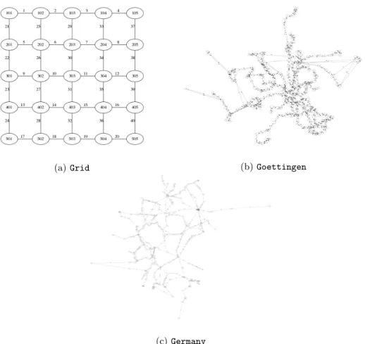
Grid: A small example first presented in [8]. It is designed to be small enough to understand effects of decisions but still contains a realistic demand structure. It has 25 stops, 40 edges and 2546 passengers. For a representation of the infrastructure, see Fig. 2a. The instance has been tackled by several researchers and can be downloaded at [12].

Goettingen: An instance based on the bus network in G¨ottingen, a small city in the geographical center of Germany. It contains 257 stops, 548 edges and 406146 passengers. For a representation of the infrastructure, see Fig. 2b.

Germany: An instance based on the long-distance rail system in Germany. It contains 250 stops, 326 edges and 3147382 passengers. For a representation of the infrastructure, see Fig. 2c.

All experiments are done using the LinTim-software framework [9, 16]. We computed a line concept without system headway as well as for every system headway from 2 to 10 while optimizing the given line planning problem.

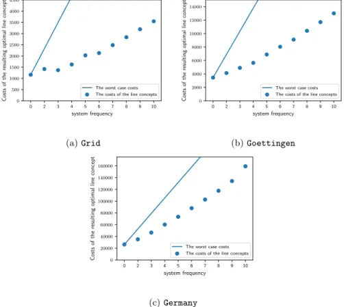
First, we consider solving the cost model discussed in Section 4. An evaluation containing the costs of the different solutions and the worst case costs of Lemma 10 can be found in Fig. 3.

There are mainly two things to observe here: First of all, the assumption that higher system headways lead to higher costs is often, but not always true. In all but one case, the costs are strictly increasing for increasing system headways.

But, as was seen in Section 3, this does not always have to be the case. This can be observed in Fig. 3a where the solution for a system headway ofi = 3 has lower costs than the solution for a system headway ofi= 2. This occurs in

(12)

(a)Grid (b)Goettingen

(c)Germany

Figure 2: Infrastructure networks of the used instances

(13)

0 2 3 4 5 6 7 8 9 10 system frequency

0 500 1000 1500 2000 2500 3000 3500 4000 4500

Costsoftheresultingoptimallineconcept

The worst case costs The costs of the line concepts

(a)Grid

0 2 3 4 5 6 7 8 9 10

system frequency 0

2000 4000 6000 8000 10000 12000 14000

(b)Goettingen

0 2 3 4 5 6 7 8 9 10

system frequency 0

20000 40000 60000 80000 100000 120000 140000 160000

(c)Germany

Figure 3: Solutions for the Cost Model

(14)

40000 42000 44000 46000 48000 50000 52000 54000

Numberofdirecttravellers

(a)Goettingen

0 2 3 4 5 6 7 8 9 10

system frequency 850000

900000 950000 1000000 1050000 1100000 1150000

Numberofdirecttravellers

(b)Germany Figure 4: Solutions for the Direct Travelers Model

cases where the demand on most edges can be met by lines with a frequencies of three. Then a system headway of i= 2 leads either to more lines or to line frequencies of four.

Additionally, note that the worst case factor for using a system headway from Lemma 10 is not obtained in practice but the difference to the theoretical bound decreases with increasing instance size.

Next, we consider the case of a passenger-oriented line planning model. We chose the direct travelers model of [4], see also Section 5. For this, we set a budget to examine the effect of the system headway on a restricted problem.

In Fig. 4 we can clearly see the effects of the system headway.

In the instanceGoettingen (Fig. 4a), we again observe that the quality of the line plan decreases most of the times with increasing system headway but there may be cases where a bigger system headway can use the given budget a little bit better, resulting in a better plan for the passenger. Hence, monotonicity of the objective function is also here likely, but not guaranteed.

In the instanceGermany(Fig. 4b), we see the effect of a late drop-off of the quality, resulting from a budget that is big enough to not be restrictive for the first few cases.

It has been recognized in several publications [3, 19, 13] that line planning should not be treated isolated from other planning stages, but an integrated approach is needed. We are hence interested not only in the effects a system headway has on line plans, but also consider if there are effects on the resulting timetable. Note that the line plan influences the resulting passengers’ travel time obtained by the timetable significantly [8, 9].

To consider the results of system headways on the timetable, we compute a periodic timetable for each of the line plans and compare their qualities, evaluating theperceived travel time of the passengers in the timetable, i.e., the travel time including a small penalty for every transfer. For the computation of

(15)

50 51 52 53 54 55

Perceivedtraveltime(min)

(a)Goettingen

0 2 3 4 5 6 7 8 9 10

system frequency 174

175 176 177 178 179 180 181 182 183

Perceivedtraveltime(min)

(b)Germany Figure 5: Evaluation of the Timetables

the timetable, we use the fastMATCH approach introduced in [15]. The results are depicted in Fig. 5.

Again, we see the anticipated results: A higher system headway results in a public transport supply with shorter headways. This leads in many cases to shorter transfer waiting times and reductions in the perceived travel time, indi- cating a higher quality for the passengers. However, also here, this interrelation does not apply without exception as Fig. 5 shows.

7 Outlook

We added the system headway constraint to line planning models, derived theoretical bounds on their effects and examined the results on practical instances for a cost model and a passenger-oriented model. It would be interesting to see the proposed system headway adjustments implemented into even more line planning models to further extend the comparison and examine the effects on public transport systems.

Another interesting topic is the evaluation of the impact of a system headway on passengers. Important metrics, such as the memorability of a timetable, can only be measured inadequately using the state-of-the-art mathematical evaluation systems and can therefore not be compared conclusively. One way of evaluating the impacts is to estimate the changes in public transport travel demand. This requires a mode choice model, which captures not only travel time and number of transfers as indicators for service quality, but also the service frequency and the regularity. This can be achieved by an indicator adaption time, which quantifies the time difference between the desired departure time of a traveler and the provided departure time of the public transport supply.

In car transport the adaption time is always zero. A public transport supply with regular and short headways reduces adaption time and thus makes public transport more competitive. Experiments with the grid instance indicate that

(16)

especially in networks with low demand the additional costs of a system headway can partially be compensated by a shift from car to public transport. In networks where high demand leads to solutions with headways below 10 minutes, the impact of a system headway on additional cost and demand is smaller. Here the modal share primarily depends on differences in in travel time and travel costs. Future work is necessary to better understand the impact of regularity and adaption time on passengers travel behavior.

References

[1] R. Bornd¨orfer, M. Gr¨otschel, and M. E. Pfetsch. A column generation approach to line planning in public transport. Transportation Science, 41:123–132, 2007.

[2] Ralf Borndörfer, Oytun Arslan, Ziena Elijazyfer, Hakan Güler, Malte Renken, Güven¸c S¸ahin, and Thomas Schlechte. Line planning on path networks with application to the istanbul metrobüs. InOperations Research Proceedings 2016, pages 235–241. Springer, 2018.

[3] S. Burggraeve, S.H. Bull, R.M. Lusby, and P. Vansteenwegen. Integrating robust timetabling in line plan optimization for railway systems. Trans- portation Research C, 77:134–160, 2017.

[4] M. Bussieck. Optimal Lines in Public Rail Transport. PhD thesis, Tech- nische Universit¨at Braunschweig, 1998.

[5] M. T. Claessens, N. M. van Dijk, and P. J. Zwanefeld. Cost optimal allocation of rail passenger lines. European Journal of Operational Research, 110:474–489, 1998.

[6] MT Claessens, Nico M van Dijk, and Peter J Zwaneveld. Cost optimal allocation of rail passenger lines.European Journal of Operational Research, 110(3):474–489, 1998.

[7] H. Dienst. Linienplanung im spurgef¨uhrten Personenverkehr mit Hilfe eines heuristischen Verfahrens. PhD thesis, Technische Universit¨at Braun- schweig, 1978. (in German).

[8] Markus Friedrich, Maximilian Hartl, Alexander Schiewe, and Anita Sch¨obel. Angebotsplanung im oeffentlichen Verkehr-Planerische und al- gorithmische Loesungen. In HEUREKA’17: Optimierung in Verkehr und Transport, 2017.

[9] M. Goerigk, M. Schachtebeck, and A. Sch¨obel. Evaluating line concepts using travel times and robustness: Simulations with the lintim toolbox.

Public Transport, 5(3), 2013.

[10] Marc Goerigk and Marie Schmidt. Line planning with user-optimal route choice. European Journal of Operational Research, 259(2):424–436, 2017.

(17)

[11] J.-W. Goossens, S. van Hoesel, and L. Kroon. On solving multi-type railway line planning problems. European Journal of Operational Research, 168(2):403–424, 2006. Feature Cluster on Mathematical Finance and Risk Management.

[12] Grid-Dataset, 2018. Downloadable at

https://github.com/FOR2083/PublicTransportNetworks.

[13] H. Huang, K. Li, and P. Schonfeld. Metro timetabling for time-varying passenger demand and congestion at stations. Technical report, Beijing Jiaotong University, 2018.

[14] Konstantinos Kepaptsoglou and Matthew Karlaftis. Transit route network design problem. Journal of transportation engineering, 135(8):491–505, 2009.

[15] J. P¨atzold and A. Sch¨obel. A Matching Approach for Periodic Timetabling.

In Marc Goerigk and Renato Werneck, editors,16th Workshop on Algorithmic Approaches for Transportation Modelling, Optimization, and Systems (ATMOS 2016), volume 54 of OpenAccess Series in Informatics (OASIcs), pages 1–15, Dagstuhl, Germany, 2016. Schloss Dagstuhl–Leibniz-Zentrum f¨ur Informatik.

[16] A. Schiewe, S. Albert, J. P¨atzold, P. Schiewe, A. Sch¨obel, and J. Schulz.

Lintim: An integrated environment for mathematical public transport optimization. documentation. Technical Report 2018-08, Preprint-Reihe, Insti- tut für Numerische und Angewandte Mathematik, Georg-August Universität Göttingen, 2018. homepage: http://lintim.math.uni-goettingen.de/.

[17] Marie Schmidt. Integrating Routing Decisions in Public Transportation Prob- lems. Optimization and its Applications. Springer, 2014.

[18] A. Sch¨obel. Line planning in public transportation: models and methods. OR Spectrum, 34(3):491–510, 2012.

[19] A. Sch¨obel. An eigenmodel for iterative line planning, timetabling and vehicle scheduling in public transportation. Transportation Research C, 74:348–365, 2017.

[20] A. Sch¨obel and S. Scholl. Line planning with minimal transfers. In 5th Work- shop on Algorithmic Methods and Models for Optimization of Railways, number 06901 in Dagstuhl Seminar Proceedings, 2006.

[21] C.A. Viggiano. Bus Network Sketch Planning with Origin-Destination Travel Data. PhD thesis, Massachusetts Institute of Technology, 2017.

[22] Vukan R Vuchic. Urban transit: operations, planning, and economics. John Wiley & Sons, 2017.

[23] Vukan R Vuchic, Richard Clarke, and Angel Molinero. Timed transfer system planning, design and operation. Departmental Papers (ESE), 1981.

(18)