The Spatial Random Effects and the Spatial Fixed Effects Model: The Hausman Test in a Cliff and Ord Panel Model

IHS Economics Series Working Paper 229

October 2008

The Spatial Random Effects and the Spatial Fixed Effects Model: The Hausman Test in a Cliff and Ord Panel Model

Jan Mutl

Michael Pfaffermayr

Impressum Author(s):

Jan Mutl, Michael Pfaffermayr Title:

The Spatial Random Effects and the Spatial Fixed Effects Model: The Hausman Test in a Cliff and Ord Panel Model

ISSN: Unspecified

2008 Institut für Höhere Studien - Institute for Advanced Studies (IHS) Josefstädter Straße 39, A-1080 Wien

E-Mail: o ce@ihs.ac.at ffi Web: ww w .ihs.ac. a t

All IHS Working Papers are available online: http://irihs. ihs. ac.at/view/ihs_series/

This paper is available for download without charge at:

The Spatial Random Effects and the Spatial Fixed Effects Model:

The Hausman Test in a Cliff and Ord Panel Model

Jan Mutl, Michael Pfaffermayr

229

Reihe Ökonomie

Economics Series

229 Reihe Ökonomie Economics Series

The Spatial Random Effects and the Spatial Fixed Effects Model:

The Hausman Test in a Cliff and Ord Panel Model

Jan Mutl, Michael Pfaffermayr October 2008

Institut für Höhere Studien (IHS), Wien

Contact:

Jan Mutl

Department of Economics and Finance Institute for Advanced Studies Stumpergasse 56

1060 Vienna, Austria : +43/1/599 91-151 email: mutl@ihs.ac.at

Michael Pfaffermayr Department of Economics University of Innsbruck Universitaetsstrasse 15 6020 Innsbruck, Austria

email: Michael.Pfaffermayr@uibk.ac.at and

Austrian Institute of Economic Research P.O.-Box 91

1103 Vienna, Austria CESIFO, Germany

Founded in 1963 by two prominent Austrians living in exile – the sociologist Paul F. Lazarsfeld and the economist Oskar Morgenstern – with the financial support from the Ford Foundation, the Austrian Federal Ministry of Education and the City of Vienna, the Institute for Advanced Studies (IHS) is the first institution for postgraduate education and research in economics and the social sciences in Austria.

The

aims to share “work in progress” in a timely way before formal publication. As usual, authors bear full responsibility for the content of their contributions.

Das Institut für Höhere Studien (IHS) wurde im Jahr 1963 von zwei prominenten Exilösterreichern –

dem Soziologen Paul F. Lazarsfeld und dem Ökonomen Oskar Morgenstern – mit Hilfe der Ford-

Stiftung, des Österreichischen Bundesministeriums für Unterricht und der Stadt Wien gegründet und ist

somit die erste nachuniversitäre Lehr- und Forschungsstätte für die Sozial- und Wirtschafts-

wissenschaften in Österreich. Die Reihe Ökonomie bietet Einblick in die Forschungsarbeit der

Abteilung für Ökonomie und Finanzwirtschaft und verfolgt das Ziel, abteilungsinterne

Diskussionsbeiträge einer breiteren fachinternen Öffentlichkeit zugänglich zu machen. Die inhaltliche

Abstract

This paper studies the spatial random effects and spatial fixed effects model. The model includes a Cliff and Ord type spatial lag of the dependent variable as well as a spatially lagged one-way error component structure, accounting for both heterogeneity and spatial correlation across units. We discuss instrumental variable estimation under both the fixed and the random effects specification and propose a spatial Hausman test which compares these two models accounting for spatial autocorrelation in the disturbances. We derive the large sample properties of our estimation procedures and show that the test statistic is asymptotically chi-square distributed. A small Monte Carlo study demonstrates that this test works well even in small panels.

Keywords

Spatial econometrics, panel data, random effects estimator, within estimator, Hausman test

JEL Classification

C21, C23

Contents

1 Introduction 1 2 The Spatial Panel Model 2 3 The Estimation of Spatial Panel Models 5

3.1 The Spatial Random Effects Estimator ... 6 3.2 The Spatial Within Estimator ... 9

4 Feasible Estimation 12 5 Hausman Specification Test 14 6 Monte Carlo Evidence 16 7 Conclusions 19

Appendix 21

References 33

Tables 35

1 Introduction ^∗

The panel literature offers the random effects and the fixed effects model to account for heterogeneity across units. While the random effects estima- tor is more efficient than the fixed effects estimator, in many non-spatial empirical applications the random effects model is rejected in favour of the fixed effects model. Often there are plausible arguments that the explanatory variables are correlated with unit specific effects. For example, in earnings equations unobserved ability of individuals may be reflected in both the unit specific effects and the explanatory variables such as the years of schooling.

The estimation of gravity equations to model bilateral trade flows is another important example where the assumptions of the random effects model are often found to be violated.

It is perfectly sensible that this issue also comes up in spatial panel models.

This paper contributes to the literature by introducing a spatial gener- alized methods of moments estimator for panel data models with Cliff and Ord type spatial autocorrelation and one-way error components. Our work complements the seminal paper of Kapoor, Kelejian and Prucha (2007) who provide a spatial generalized least squares (spatial GLS) estimator for the spatial random effects model. In addition to their work, our model allows for an endogenous spatial lag of the dependent variable. We discuss the proper instrumentation of the endogenous spatial lag and suggest an instrumental variable (IV) procedure for both the spatial within estimator and the spatial GLS estimator. In order to discriminate between the two spatial panel mod- els, we also propose a Hausman test that accounts for spatially autocorrelated disturbances. Specifically, we derive the joint asymptotic distribution of the spatial GLS and the spatial within estimators, as well as the asymptotic dis- tribution of the spatial Hausman test for random versus fixed effects. This test should enable applied researchers to choose between these two models, when spatial correlation of the endogenous variable and/or the disturbances is present.

Our paper is not the first that considers spatial within or fixed effects estimators. Case (1991) seems to be among the first in estimating spatial random and fixed effects models. Korniotis (2008) introduces a bias-corrected estimator for a spatial dynamic panel model with fixed effects. Lee and

∗

We would like to thank Robert Kunst and Ingmar Prucha for helpful comments and suggestions.

1

See also the papers cited in Baltagi (2008) for more examples.

Yu (2008) establish the asymptotic properties of quasi-maximum likelihood estimators for fixed effects spatial autoregressive (SAR) panel data models with SAR disturbances, where the time periods and/or the number of spatial units can be finite or large in all combinations except that both are finite (see also Yu, de Jong and Lee, 2006 and 2007).

In the next section we specify our model and spell out the maintained assumptions. Section 3 defines the two estimators under consideration and shows that the random effects and the within estimators are jointly asymp- totically normally distributed under the random effects assumption. Section 4 introduces the feasible counterparts of the considered estimators based on an initial instrumental variable estimator. We show that the initial estimator is consistent and asymptotically normal and derive its asymptotic distribu- tion. We also demonstrate that true and feasible estimators have the same asymptotic distribution. Section 5 defines the spatial Hausman test that al- lows to discriminate between the two spatial panel models. It provides its asymptotic distribution under the null and also shows that the test statistics diverges in probability under the alternative hypothesis. In Section 6 we report the results of Monte Carlo experiments that assess both the size and the power of the proposed spatial Hausman test in finite samples. Finally, the last section concludes.

2 The Spatial Panel Model

Consider the following spatial panel model:

y

= λ

j=1

w

y

+ x

β + α + u

. (2.1) Index i = 1, .., N denotes the cross-sectional dimension of the panel. The index t = 1, ..., T refers to the time series dimension of the panel and y

is the (scalar) dependent variable.

j=1

w

y

denotes the spatial lag of the dependent variable with w

being observable non-stochastic spatial weights. x

is a 1 × K − 1 vector of exogenous variables, β is a K − 1 × 1 parameter vector, λ a scalar parameters and α refers to the constant. u

is the overall disturbance term.

We allow for cross-sectional sectional correlation of the disturbances and,

in particular, we assume that the disturbances follow a Cliff and Ord type

spatial autocorrelation (SAR(1) in terminology of Anselin, 1988) as proposed by Kapoor, Kelejian and Prucha (2007):

u

= ρ

j=1

m

u

+ ε

, (2.2) where ρ is a scalar parameter and m

are observable spatial weights (pos- sibly the same as the weights w

). The innovations ε

have the following one-way error component structure:

ε

= µ

+ ν

. (2.3) ν

are independent innovations and µ

are individual effects, which can be either fixed or random.

We index all variables by the sample size N, since they form triangular arrays. This is necessary because the model involves inverses of matrices whose size depends on N , and hence their elements must change with N . Thus at the minimum y

and u

are triangular arrays in the present specification.

We sort the data so that the fast index is i and the slow index is t.

Stacking the model over the N cross-sections for a single period t yields y

= λW

y

+ X

β + αι

+ u

, (2.4) u

= ρM

u

+ ε

,

ε

= µ

+ ν

where ι

is a (N × 1) vector of ones and

y

=



  y

...

y



  , X

=



  x

...

x



  , u

=



  u

...

u



  (2.5)

ε

=



  ε

.. . ε



  , ν

=



  ν

.. . ν



  , µ

=



  µ

.. . µ



  ,

W

=



 

w

· · · w

.. . . .. .. . w

· · · w



  , M

=



 

m

· · · m

.. . . .. .. . m

· · · m



  .

Stacking over time periods, we write our model compactly as

y

= λ W

y

+ X

β + αι

+ u

(2.6)

= Z

δ + u

, u

= ρ M

u

+ ε

,

ε

= (ι

⊗ I

) µ

+ ν

.

where W

= (I

⊗ W

), M

= (I

⊗ M

), Z

= (ι

, W

y

, X

), δ = (α, λ, β

)

, ι

is an T × 1 vector of ones, ι

is a N T × 1 vector of ones and

y

=



  y

...

y



  , X

=



  x

...

x



  , u

=



  u

...

u



  , (2.7)

ε

=



  ε

...

ε



  , ν

=



  ν

...

ν



  .

Throughout we maintain the following basic assumptions, which follow closely those postulated in Kapoor, Kelejian and Prucha (2007).

Assumption 1

The elements of ν

are independently and identically distributed with finite absolute 4 + δ

moments for some δ

> 0. Furthermore, E ν

= σ

> 0.

Assumption 2

The spatial weights collected in M

and W

are non-stochastic and (a) m

= 0 and w

= 0.

(b) The absolute row and column sums of the matrices M

, W

, (I

− ρM

)

, (I

− λW

)

are uniformly bounded in absolute value, i.e.

i=1

| a

|

≤ k < ∞ , where k does not depend on N (but may depend on para- meters of the model, i.e. on ρ or λ, respectively) and a

denotes elements of the above matrices.

(c) | ρ | ≤ k

< 1/λ

(M

), | λ | ≤ k

< 1/λ

(W

), where λ

(.) de- notes the largest absolute eigenvalue of a matrix.

(d) The matrices (I

− ρM

) and (I

− λW

) are non-singular.

Assumption 3

The exogenous variables collected in X

are non-stochastic and vary with both individuals and time. Their elements are uniformly bounded in absolute value.

Assumption 1 is a restriction on the higher moments of the disturbances required for asymptotic results. Assumption 2(a) is a typical normalization (but is not necessary for our asymptotic results). Assumptions 2(b) and (c) are satisfied in many empirical applications and hold, for example, if the spatial weights matrices W

and M

are (maximum)-row normalized and

| λ | ≤ k

< 1 and | ρ | ≤ k

< 1, respectively. Observe that Assumption 2(d) follows from 2(c).

Assumptions like 2(b) - 2(d) are typically maintained in spatial models (see Kelejian and Prucha, 1999) and restrict the extent of spatial dependence among cross-section units. It will be satisfied if the spatial weighting matrix is sparse so that each unit possess a limited number of neighbors or if the spatial weights decline sufficiently fast in distance.

3 The Estimation of Spatial Panel models

In their seminal paper Kapoor, Kelejian and Prucha (2007) concentrate on the random effects model, assuming that the explanatory variables and the unit specific error terms are independent. Yet, in applied work exactly this assumption often does not hold and a fixed effects specification is employed instead. Examples in a non-spatial setting, where the unit specific effects and the explanatory variables may be correlated include earnings equations.

In this setting the unobserved individual ability of an individual is typically correlated with the years of schooling, which enters the earnings equation as explanatory variables (see e.g. Baltagi, 2008, p. 79). Also in models ex- plaining bilateral trade flows, the random effects model is typically rejected in favour of the fixed effects model to mention another example (see Egger, 2000). In addition, the considered spatial panel model allows for an endoge- nous spatial lag. First, we analyze the spatial random effects estimator for this general spatial panel model.

2

This follows from Corrolary 5.6.16 in Horn and Johnsonn (1985) using their Lemma

5.6.10.

3.1 The Spatial Random Effects Estimator

Under the random effects specification, the unit specific effects µ

are as- sumed to be random and the following standard assumption is maintained.

Assumption 4 (RE)

The elements of µ

are independently and identically distributed with finite absolute 4 + δ

moments for some δ

> 0 and E µ

= σ

> 0. Fur- thermore, the elements of µ

are independent of the process for ν

and E µ

| X

= 0 for all i and t.

Under Assumptions 1, 2 and 4 (RE), it follows that the disturbances are generated as

u

= (I

− ρ W

)

ε

. (3.1) Hence, under the random effects specification, the variance covariance matrix of the disturbances is given by

Ω

= E (u

u

) (3.2)

= (I

− ρ M

)

σ

(ι

ι

⊗ I

) + σ

I

(I

− ρ M

N

)

. It proves to be useful to use the notation σ

= T σ

+ σ

and define the following standard within and between transformation matrices Q

(i = 0, 1):

Q

= I

−

J

⊗ I

(3.3)

Q

=

J

⊗ I

,

where J

is a T × T matrix of unit elements. The matrices Q

are the standard transformation matrices utilized in the error component literature but adjusted for the different stacking of the data (compare Kapoor, Kelejian and Prucha, 2007 and Baltagi, 2008). The matrices Q

are symmetric and idempotent and mutually orthogonal. The variance covariance matrix of the disturbances can then be written as (see Baltagi, 2008, p. 18)

Ω

= (I

− ρ M

N

)

Ω

(I

− ρ M

N

)

, (3.4) where

Ω

= E (ε

ε

) = σ

Q

+ σ

Q

. (3.5)

Furthermore, the inverse of Ω

can then be expressed as Ω

= (I

− ρ M

) Ω

(I

− ρ M

N

) , where

Ω

= σ

Q

+ σ

Q

. (3.7) If the parameter values ρ, σ

and σ

(and, therefore, σ

) are known, the efficient GLS estimation procedure is to transform the model by the square root of the inverse of the variance-covariance matrix of the disturbances

σ

Ω

= σ

Ω

(I

− ρ M

) . (3.8) This is equivalent to first applying the spatial counterpart of the Cochrane- Orcutt transformation (I

− ρ M

) that eliminates the spatial correlation from the disturbances and then the familiar panel GLS transformation σ

Ω

that accounts of the variance-covariance structure of the innovations induced by the random effects. To simplify the exposition, we collect the parameters of the variance covariance matrix in a vector ϑ = (ρ, σ

, σ

) and use the no- tation Ω

(ϑ) to explicitly note the dependence of the GLS transformation on these parameters. Observe that in a balanced panel the order with which the transformations are applied is irrelevant (see also Remark A1 in Kapoor, Kelejian and Prucha, 2007).

Since the spatial lag W

y

is endogenous in the (transformed) model, we adapt the instrumental variable procedure described in Kelejian and Prucha (1998).

Specifically, we first eliminate the spatial correlation eliminated from the error term using the Cochrane-Orcutt transformation. Then we ap- ply the instrumental variable procedure for random effects models suggested by Baltagi and Li (1992), Cornwell, Schmidt and Wyhowsky (1992) and sur- veyed by Baltagi (2008). These authors show in a non-spatial setting that the optimal set of instruments for a random effects model with endogenous variables is comprised of [Q

X

, Q

X

, ι

]. Observe that

E[ y

] = ( I

− λ W

)

( X

β + αι

) (3.9)

=

k=0

λ

W

N

(X

β + αι

) ,

3

It is possible to use other sets of instruments, such as those proposed in Lee (2003) or

Kelejian, Prucha and Yuzefovich (2004).

where W

N

= I

. Hence under the present assumptions, the ideal set of instruments is based on

σ

Ω

(ϑ) W

E[y

] = σ

k=0

λ

Ω

(ϑ) W

N

(X

β + αι

) (3.10)

=

k=0

λ

(Q

+

Q

) W

N

(X

β + αι

)

− ρ

k=0

λ

(Q

+

1

Q

) M

N

W

N

(X

β + αι

) Therefore, the transformed endogenous variable σ

Ω

(ϑ) W

N

y

is best instrumented by

H

= [H

, H

] (3.11)

= [Q

G

, Q

G

] ,

where G

contains a subset of the the linearly independent columns of X

, W

X

, W

N

X

..., M

X

, M

W

X

, M

W

N

X

, ...

and G

contains a subset of the the linearly independent columns of G

, ι

, M

ι

, M

W

ι

, M

W

N

ι

...

.

The columns in G

and G

must be chosen so that the columns of H

are linearly independent. In the special case where W

= M

the set of instruments is based on G

= [X

, W

X

, W

N

X

, ...] and G

= [G

, ι

, W

ι

, ...] . If the spatial weighting matrices are row normalized, the set of instruments in G

includes only ι

besides G

, since in this case M

ι

= W

ι

= ι

.

In the following we assume that the NT × p matrix of instruments de- noted by H

is of the form described above. In order to derive asymptotic properties of the considered estimators, we maintain the following additional assumption for the matrix of instruments and the explanatory variables of the model collected in Z

= [ι

, W

y

, X

]:

Assumption 5

Let Z

(ϑ) = Ω

(ϑ) Z

. The matrix of instruments H

has full column

rank and consists of a subset of linearly independent columns of [Q

G

,

Q

G

]. Furthermore, it satisfies the following conditions:

(a) M

= lim

(N T)

H

H

exists and is finite and non-singular, (b) M

RZ

= p lim

(N T )

H

Z

exists and is finite with full column rank.

The spatial random effects estimator of δ = (α, λ, β

)

is then defined as δ

=

Z

(ϑ)

Z

(ϑ)

Z

N

(ϑ) y

(ϑ) , (3.14) with Z

(ϑ) = P

Z

(ϑ), Z

(ϑ) = Ω

(ϑ) Z

and y

(ϑ) = Ω

(ϑ) y

. P

= H

H

H

H

is the projection matrix based on the in- struments H

.

The joint asymptotic distribution of the spatial random effects estimator and the spatial within estimator under known nuisance parameter vector ϑ is given in Theorem 1 below. This theorem is based on the random effects Assumption 4 (RE) and forms the basis of the Hausman test. The asymptotic properties of this test and its feasible counterparts are given in Theorem 2 in Section 5.

3.2 The Spatial Within Estimator

As an alternative to the random effects assumption above, the spatial within estimator allows for possible correlation of the unit specific effects and the explanatory variables. We follow Mundlak (1978) and maintain the following fixed effects assumption:

Assumption 6 (FE)

The vector individual effects is given by

µ

= (I

− ρ M

)Q

Z

π + ξ

,

where π = 0 and the elements of the random vector ξ

satisfy Assumption 4 (RE).

We can redefine the innovations of the model under the fixed effect as- sumption to be

ε

= (ι

⊗ I

) ξ

+ ν

, (3.15)

i.e. replace the individual effects µ

with only their independent compo- nent ξ

. Observe that the fixed effects assumption then implies that the disturbances of the model are given by

u

= (I

− ρ M

)

ε

+ Q

Z

π. (3.16) Clearly, the explanatory variables are uncorrelated with the individual effects if and only if π = 0 and the random effects model defined under (4) (RE) arises as a special case of (6) (FE). Under Assumption 6 (FE) with π = 0 the spatial GLS estimator is inconsistent. However, one can apply the within transformation Q

to wipe out the individual effects (see e.g. Baltagi, 2008 and Mundlak 1978). Using Q

(I

− λ M

) = (I

− λ M

) Q

, one obtains

Q

u

= (E

⊗ I

) (ρ (I

⊗ M

) u

+ Q

Z

π+ (ι

⊗ I

) µ

+ ν

) ,

= ρ (I

⊗ M

) (E

⊗ I

)u

+ (E

⊗ I

)ν

= ρ (I

⊗ M

) Q

u

+ Q

ν

. (3.17) or

Q

u

= (I

− λ M

)

Q

ν

where E

= I

−

J

. Hence, one can apply the Cochrane-Orcutt type transformation on the within transformed model to obtain the fixed effects generalized least squares (FEGLS) estimator.

More importantly, one can base the method of moment estimator of (ρ, σ

) on the initial within transformed residuals of the initial within estimator as given by Q

u

, which are consistently estimated under both the spatial random effects model and the spatial fixed effects model. Obviously, the set of instruments denoted by H

now comprises the linear independent columns of Q

G

. Since the constant is wiped out in the spatial within estimator, we define the (K × K ) matrix Z

= Q

[ W

y

, X

] with the corresponding (K × 1) parameter vector θ = (λ, β

)

.

In order to derive the asymptotic properties of the spatial within esti- mator, we maintain the following additional assumptions for the matrix of instruments used in the spatial within model:

Assumption 7

Let Z

= Q

[ W

y

, X

]. The matrix of instruments H

has full

column rank and consists of a subset of linearly independent columns of

Q

G

. Furthermore, it satisfies the following conditions:

(a) M

= lim

(NT )

H

H

is finite and non-singular with full column rank.

(b) M

= p lim

(NT )

H

(I

− ρ M

) Z

exists and is finite with full column rank.

Again, treating ρ as known, we apply the Cochrane-Orcutt type transforma- tion to the within transformed model yielding:

Q

(I

− ρ M

) y

= (I

− ρ M

) Q

y

(3.18)

= ( I

− ρ M

) Q

Z

+ Q

ν

y

(ρ) = Z

(ρ) θ + ν

,

where

y

(ρ) = (I

− ρ M

) Q

y

, (3.19) Z

(ρ) = (I

− ρ M

) Z

ν

= Q

ν

.

The spatial within estimator is then obtained by applying IV to the trans- formed model to obtain

θ

=

Z

(ρ)

Z

(ρ)

Z

(ρ)

y

(ρ) , (3.20) with

Z

(ρ) = P

Z

(ρ) (3.21)

= P

(I

− ρ M

) Z

, where P

= H

H

H

H

is the projection matrix based on the instruments H

.

The following theorem establishes our main asymptotic result concern- ing the common asymptotic distribution of the spatial random effects and the spatial within estimators under random effects Assumption 4 (RE). The Hausman test for spatial panels derived below will be based on this re- sult. Since the random effects estimator includes the constant, we define δ

=

α

, θ

.

Theorem 1 Let Assumptions 1-5 and 7 hold. Then

√ N T

θ

− θ θ

− θ

→

N

0,

Σ

Σ

Σ

Σ

,

where Σ

= σ

M

M

QH_Q

M

and Σ

is the lower-right K × K block of the matrix σ

M

HRZ

M

M

RZ

. Proof: See the Appendix.

4 Feasible Estimation

The spatial GLS and spatial within estimators defined above are based on the unknown parameters ρ, σ

and σ

which have to be estimated. The feasible estimation procedure starts by estimating the within transformed model using the instruments H

= Q

G

as described above to obtain initial within IV estimates. This initial estimator is consistent under both the random effects and the fixed effects specification (see Baltagi, 2008) and it can be written as

θ

=

Z

Q

Z

Z

Q

y

, (4.22) where Z

= P

Q

Z

. The following proposition gives the asymp- totic distribution of the initial estimator.

Proposition 1 Let the limit M

= p lim

(NT )

H

Z

exist and be finite with full column rank. Let Assumptions 1-3, 7 and either 4 (RE), or 6 (FE) hold. Then

√ NT

θ

− θ

→ N (0, Σ

) , where Σ

= σ

M

M

M

.

Proof: See the Appendix.

The projected residuals then give consistent initial estimates of Q

u

which can be used in the spatial generalized moments (GM) estimator as suggested by Kapoor, Kelejian and Prucha (2007). These authors use OLS residuals, which are consistent under the random effects assumption 4 (RE) but would be biased under the fixed effects assumption 6 (FE). The spa- tial GM estimator for ρ, σ

can then be based on the first three moment conditions given in Kapoor, Kelejian and Prucha (2007).

Using Q

M

= M

Q

and the notation ε

= M

ε

, we can formulate the first three moment conditions in terms of Q

u

as

E



 

1

N(T−1)

ε

Q

ε

1

N(T−1)

ε

Q

ε

N(T−1)

ε

Q

ε



  (4.23)

=



 

1

N(T−1)

u

Q

(I

− ρ M

N

) (I

− ρ M

) Q

u

1

N(T−1)

u

Q

(I

− ρ M

N

) M

N

M

(I

− ρ M

) Q

u

1

N(T−1)

u

Q

(I

− ρ M

N

) M

N

(I

− ρ M

) Q

u



 

=



 σ

σ

tr( M

N

M

) 0





Under the random effects model, Assumption 4 (RE), we add a fourth mo- ment condition.

E

N

ε

Q

ε

(4.24)

=

N

u

Q

(I

− ρ M

N

) (I

− ρ M

) Q

u

= σ

With the solution of the first three moment conditions at hand, one can

solve the fourth moment condition to obtain an estimate of σ

. Theorem 1

in Kapoor, Kelejian and Prucha (2007, p. 108 ) shows that the estimators

for ρ, σ

and σ

based on these moment conditions and some additional

assumptions (see their Assumption 5) are consistent as long as the initial

estimator θ

is consistent. Note, that this is the case for the spatial within

estimator under both the Assumption 4 (RE) and Assumption 6 (FE).

Proposition 2 demonstrates that the parameters ρ, σ

and σ

are nui- sance parameters and that the feasible spatial random effects and the feasi- ble spatial within estimates have the same asymptotic distribution as their counterparts based on the true values of ρ, σ

and σ

.

Proposition 2 Let the feasible estimators θ

and θ

be based on consistent estimators of ρ, σ

, and σ

. Then under Assumptions 1-5 and 7 we have

√ N T

θ

− θ

→ 0,

√ N T

θ

− θ

→ 0.

Proof: See the Appendix.

5 Hausman Specification Test

The spatial within estimator is consistent under both the random effects as- sumption 4 (RE) and the fixed effects assumption 6 (FE) since it wipes out the unit specific effects by applying the within transformation. The criti- cal assumption for the validity of the spatial random effects model is that E (u

| X

) = 0, implying that the spatial random effects model is inconsis- tent under the fixed effects Assumption 6 (FE). The Hausman test (Hausman, 1978) suggests comparing these two estimators and to test whether the ran- dom effects assumption maintaining E (u

| X

) = 0 holds true. The spatial GLS estimator of the random effects model is more efficient than the spatial within estimator under the random effects assumption 4 (RE). Moreover, un- der H

both considered estimators are consistent, while under H

the spatial random effects estimator is inconsistent, but the spatial within estimator is consistent.

The theorem below defines the Hausman test statistic for spatial panels and provides its asymptotic distribution under the null.

Theorem 2 Under Assumptions 1-5 and 7, we have

(a) √

NT

θ

− θ

→ N (0, Σ

− Σ

) ,

where Σ

− Σ

is positive definite.

(b)

Σ

− Σ

→

Σ

− Σ

where

Σ

= σ

NT

Z

(I

− ρ

M

N

) P

(I

− ρ

M

) Z

, and

Σ

= σ

N T

Z

Ω

ϑ

P

Ω

ϑ

Z

,

with ϑ

= ρ

, σ

, σ

being some consistent estimator of ϑ.

(c) Let

H

= N T

θ

− θ

Σ

− Σ

θ

− θ

,

and

H

= NT

θ

− θ

( Σ

− Σ

)

θ

− θ

.

H

− H

→

0, where H

is asymptotically χ

distributed with K degrees of freedom.

Proof: See the Appendix.

Given Theorem 2 in Kapoor, Kelejian and Prucha (2007) and the results in this paper, a feasible estimation and testing procedure can be summa- rized as follows. First calculate a consistent initial instrumental variables estimator θ

which ignores the spatial correlation in the disturbances and wipes out the individual effects using the within transformation. Second, use the resulting estimated disturbances in a spatial GM procedure as described in Kapoor, Kelejian and Prucha (2007) and obtain a (consistent) estimator ϑ

= ρ

, σ

, σ

. Third, transform the model by the spatial Cochrane-

Orcutt transformation and then either the within or the GLS transformation

to obtain the spatial GLS and spatial within estimators θ

and θ

.

Finally, calculate the Hausman test statistics H

and use it to make a deci-

sion whether the random or fixed effects specification is more appropriate.

Under the alternative Assumption 6 (FE) one obtains δ

=

Z

(ϑ)

Z

(ϑ)

Z

N

(ϑ) y

(ϑ)

= δ +

Z

(ϑ)

Z

(ϑ)

Z

N

(ϑ) σ

Ω

· Q

Z

(ϑ) π + (ι

⊗ I

) µ

+ ν

while

θ

=

Z

(ρ)

Z

(ρ)

Z

(ρ)

y

(ρ)

= δ +

Z

(ρ)

Z

(ρ)

Z

(ρ)

Q

ν

remains the same as under H

. The following Proposition shows that the Hausman test statistic is a consistent statistic, i.e., the power of the test approaches unity as N → ∞ for an arbitrary significance level of the test.

Proposition 3 Let Assumptions 1-3 and 5-7 hold and let γ > 0 be some positive constant. Then lim

P (H

> γ) = 1.

Proof: See the Appendix

6 Monte Carlo Evidence

The Monte Carlo analysis investigates the small sample properties of the proposed spatial Hausman test. For this we use a simple spatial panel model that includes one explanatory variable and a constant:

y

= βx

+ α + u

, i = 1, ..., N and t = 1, ..., T. (6.1) We set β = 0.5 and α = 5. The explanatory variable is generated as x

= ζ

+ z

with ζ

∼ i.i.d. U [ − 7.5, 7.5] and z

∼ i.i.d. U [ − 7.5, 7.5] with U [a, b]

denoting the uniform distribution on the interval [a, b]. x

is treated as non-

stochastic variable and it is held fixed in repeated samples. The individual-

specific effects are allowed to be correlated with x

, setting µ

= µ

+ πx

,

where µ

is drawn from a normal distribution, i.e. µ

∼ i.i.d. N (0, 10φ) and

π is a constant parameter. This mimics the fixed effects assumption 2(FE) with π = 0. At π = 0 the random effects assumption 4 holds and it forms the null for the spatial Hausman test. We normalize µ

so that its mean is 0 and its variance 10φ, where φ =

2 µ

σ²_µ+σ²_ε

, 0 < φ < 1, denotes the proportion of the total variance due to the presence of the individual-specific effects. For the remainder error we assume ε

∼ i.i.d. N (0, 10(1 − φ)). This implies that total the variance of the disturbances is σ

+ σ

= 10.

The row normalized spatial weighting matrix uses a regular lattice with 144 and 324 cells, respectively, containing one observation each. The spatial weighting scheme is based on a rook design, where every unit is surrounded by four neighbors. The corresponding spatial weighting matrix is maximum- row normalized following Kelejian and Prucha (2007). We will use the same spatial weighting matrix to generate both the endogenous spatial lag and the spatial lag of the error term.

The spatial parameters λ and ρ vary over the set {− 0.8, − 0.4, 0, 0.4, 0.8 } . The parameter π takes its values in {− 0.3, − 0.2, − 0.1, 0, 0.1, 0.2, 0.3 } . Based on the discussion above we use the instruments H

= [Q

x

, Q

W

x

, Q

, W

x

], while H

is composed of [H

, Q

x

, Q

W

x

, Q

W

N

x

, ι

, Q

W

ι

].

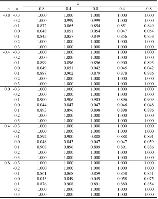
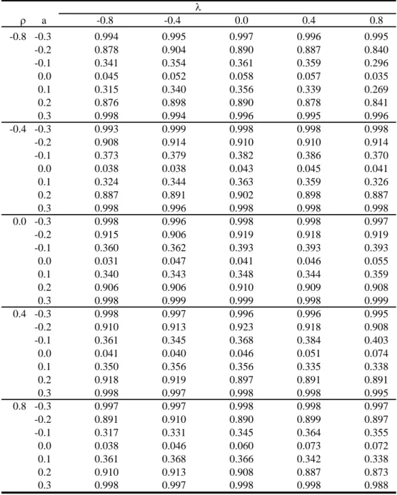
In each experiment we calculate the size of the Hausman test, which is given by the share of rejections at π = 0. The power of the spatial Hausman test is given by the share of rejections at π = 0.

===== Tables 1-4 =====

The baseline scenario is reported in Table 1 setting N = 144, T = 5 and φ = 0.5. The results show that the proposed spatial IVGLS estimators work well and that the spatial Hausman test exhibits good performance for almost all considered parameter configurations. In the experiments reported in this Table, the spatial Hausman test comes close to the nominal size of 0.05 in most of the cases. Exceptions are only observed for high values of λ, where the test is slightly oversized. For example, at λ = 0.8 and ρ = 0.8 the size of the spatial Hausman test is 0.09. At negative values of ρ, this phenomenon is not observed. The power of the test by and large remains unaffected by variations of ρ and λ, although it seems somewhat lower at high absolute values of ρ or high absolute values of λ.

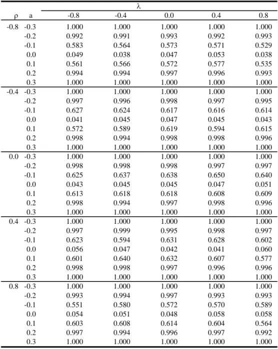
A larger cross-section (N = 324) improves both the size and the power of

the test as expected (see Table 2). The size distortion at high positive values

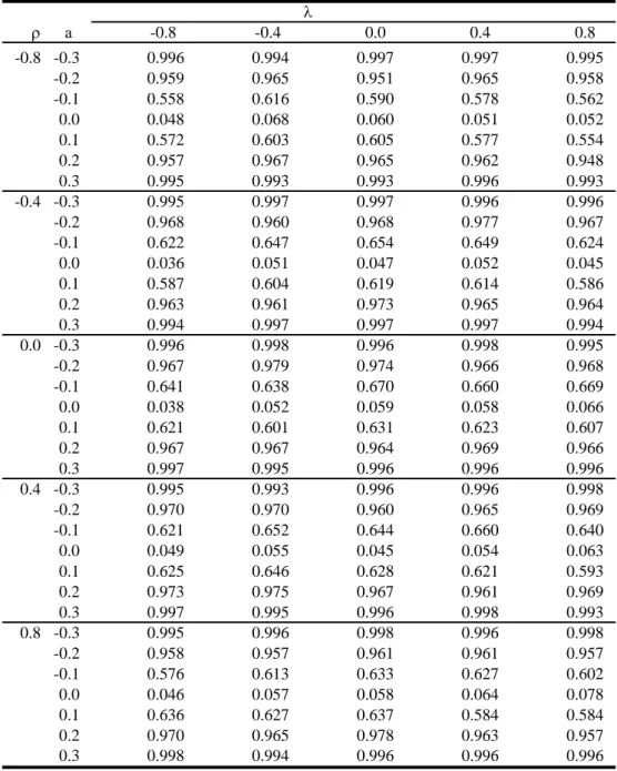
of λ is now reduced and the power of the spatial Hausman test is considerably higher. In Table 3 we extend the time series dimension and set T = 10. The size distortion at high values of λ becomes smaller as T increases and this effect seems more pronounced than in an extended cross-section as analyzed in Table 2. However, the improvement in power is much smaller as compared to extending the cross-section dimension.

In Table 4 we set N = 144 and φ = 0.8, so that σ

= 8 and σ

is 2.

With a larger weight of the variance of the unit specific effects, we observe a better performance of the spatial Hausman test in terms of its size. The size distortion observed in the baseline scenario now vanishes. Also, the power of the test is significantly higher.

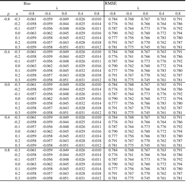
===== Tables 5-7 =====

Tables 5-7 report the root mean square error (RMSE) and the bias of the estimators of β, λ and ρ for the basic case with N = 144, T = 5 and θ = 0.5. Following Kapoor, Kelejian and Prucha (2007) we define the bias as the difference between the respective median of the parameter estimate and its true counterpart, while RMSE =

!

bias

+

. IQ is defined as the interquantile range, i.e. the difference between the 0.75 and 0.25 quantile of the simulated parameter distribution. Under a normal distribution the median and the mean coincide and

corresponds to the standard deviation (up to a rounding error).

The simulation exercises reveal a negligible bias for β and a somewhat

higher efficiency of the random effects estimator under H

. The gain in

efficiency is especially large at high positive values of λ and at high absolute

values of ρ. A similar pattern can be found for the RMSE of λ, although the

efficiency loss of the spatial within estimator is much higher as compared to

that for β. Under H

the random effects estimator is inconsistent leading to

large biases in both β and λ. The bias of the slope parameter β is hardly

affected by different degrees of spatial dependence as represented by the

parameters values of λ. However, the bias is negative at low and negative

values of ρ and turns to the positive if ρ gets high. With respect to the

estimates of λ, we find that the bias is negative if λ or ρ take on negative

values, but that it declines in λ and/or ρ. At λ = 0.8 or ρ = 0.8 the

bias nearly vanishes. The results in Table 7 indicate that the estimates of ρ

remain unaffected by deviations from H

as expected. These estimates are

based on the spatial within estimator which is consistent under both H

and H

.

We also assess the performance of the spatial Hausman test for non- normal disturbances.

In particular, we follow Kelejian and Prucha (1999) and assume lognormal remainder disturbances assuming ε

=

, where ξ

∼ i.i.d. N(0, 1). Alternatively, we maintain that the distribution of the remainder error exhibits fatter tails than the normal and ε

∼ i.i.d t(5). In both cases the performance of the spatial Hausman test is comparable to that under normal disturbances. However, under the t(5) error distribution the power of the test is smaller. Figures 1-3 summarize the Monte Carlo simulations in terms of normal probability plots pooling all experiments for the parameters of interest (β, λ and ρ) in one graph. We see considerable deviations of the simulated values from the normal both in the lower and upper tail, especially for the estimates of λ and ρ .

To summarize, the small Monte Carlo study shows that the proposed spatial Hausman test works well even in small panels. In this spatial setting, the test is able to detect deviations from the assumption that unobserved unit effects and the explanatory variables are uncorrelated, which is critical for the validity of spatial random effects models.

7 Conclusions

In this paper we study spatial random effects and spatial fixed effects mod- els. We note that in many non-spatial applications the critical assumption maintained under the random effects specification, namely that unit spe- cific effects and explanatorily variables are uncorrelated, does not hold. This seems also a possibility in a spatial setting and should be tested, since the estimates of spatial random effects are inconsistent if this assumption fails to hold.

Using a spatial Cliff and Ord type model as analyzed in Kapoor, Kelejian and Prucha (2007) but augmented by an endogenous spatial lag, we intro- duce (feasible) instrumental variables estimators for both the spatial random effects model and a spatial fixed effects model. We derive the asymptotic distributions of these estimators as well as those of their feasible counter- parts. In addition, we propose a spatial Hausman test to compare these two

4

The corresponding tables are available from the authors upon request.

models, accounting for spatial autocorrelation in the disturbances. A small

Monte Carlo study shows that this test works well even in small panels.

A Appendix

Proof of Theorem 1:

We denote the (T + 1) N × 1 vector of i.i.d.(0, 1) innovations as ζ

=

N σµ

,

and we write the stacked estimators as

δ

− δ

θ

− θ

= P

F

ζ

, (A.1)

where

P

=

P

0 0 P

, F

=

F

F

0 F

with

P

=

Z

H

H

H

H

Z

· (A.3)

Z

H

H

H

, P

=

Z

H

H

H

H

Z

· Z

H

H

H

, and

F

= σ

σ

H

Ω

(ι

⊗ I

) (A.4)

= σ

H

σν

σ1

Q

+ Q

(ι

⊗ I

) , F

= σ

H

Ω

= σ

H

σν

σ¹

Q

+ Q

, F

= σ

H

Q

.

By Assumptions (5) and (7) it follows that the sequence of the stochastic matrices (NT ) P

and (NT ) P

converge in probability, i.e.

(NT ) P

→

M

HRZ

M

RH_R

M

RZ

M

HRZ

M

RH_R

, (A.5) (NT ) P

→

M

M

QHQ

M

M

M

QHQ

.

5

We have used the properties of the Q

and Q

transformation matrices (see, e.g.

Baltagi, 2008 and Kapoor, Kelejian and Prucha, 2007, Remark A1). In particular we have

Ω

= σ

Q

+ σ

Q

.

Next we apply the central limit theorem for vectors of triangular arrays given in Theorem A1 in Mutl (2006) to (NT )

1

2

F

ζ

. By Assumptions 1 and 4, the vector of random variables ζ

satisfies the assumptions of the central limit theorem. Observe that the matrix F

is non-stochastic and that Assumptions 2, 3 and 5 imply that the row and column sums of F

are uniformly bounded in absolute value. Hence, it remains to be demonstrated that the matrix (NT )

F

F

has eigenvalues uniformly bounded away from zero.

One can show that

(F

F

)

(p+2q)×(p+2q)

= σ

H

H

H

H

H

H

H

H

(A.7)

= σ

H

0 0 H

I

I

I

I

H

0 0 H

and hence

(NT )

λ

(F

F

) ≥ min

(N T )

λ

H

H

, (NT )

λ

H

H

· λ

I

I

I

I

. (A.8)

Observe that (N T )

H

H

and (NT )

H

H

and

I

I

I

I

are symmetric. By Assumptions (3.11) and (7) the first two matrices have full rank p + q and q, respectively. Note that the third matrix has trivially full rank as well. Hence, (NT )

λ

(F

F

) is uniformly bounded away from zero. Therefore, by the central limit theorem it follows that

NT

F

ζ

→

N (0, lim

N→∞

1

NT

F

F

). (A.9)

6

Recall that the (N T × q) matrix of within transformed instruments H

= Q

G

has full column rank q and that Q

H

= H

. Furthermore, H

= [H

, H

], where H

= Q

G

with dimension (N T × p) and full column rank p. Since Q

Q

= 0 , it follows that

H

Q

H

= H

H

(A.6)

=

G

Q

G

Q

Q

H

=

0

H

H

.

7

Note that it can be demonstrated that lim

(N T)

F

F

exists.