Evolution of Mediterranean Sea water properties under climate change scenarios in the Med‑CORDEX ensemble

(1)

https://doi.org/10.1007/s00382-019-05105-4

Evolution of Mediterranean Sea water properties under climate change scenarios in the Med‑CORDEX ensemble

Javier Soto‑Navarro¹ · G. Jordá² · A. Amores¹ · W. Cabos³ · S. Somot⁴ · F. Sevault⁴ · D. Macías⁵ · V. Djurdjevic⁶ · G. Sannino⁷ · L. Li⁸ · D. Sein^9,10

Received: 14 July 2019 / Accepted: 23 December 2019

Abstract

Twenty-first century projections for the Mediterranean water properties have been analyzed using the largest ensemble of regional climate models (RCMs) available up to now, the Med-CORDEX ensemble. It is comprised by 25 simulations, 10 historical and 15 scenario projections, from which 11 are ocean–atmosphere coupled runs and 4 are ocean forced simulations.

Three different emissions scenarios are considered: RCP8.5, RCP4.5 and RCP2.6. All the simulations agree in projecting a warming across the entire Mediterranean basin by the end of the century as a result of the decrease of heat losses to the atmosphere through the sea surface and an increase in the net heat input through the Strait of Gibraltar. The warming will affect the whole water column with higher anomalies in the upper layer. The temperature change projected by the end of the century ranges between 0.81 and 3.71 °C in the upper layer (0–150 m), between 0.82 and 2.97 °C in the intermediate layer (150–600 m) and between 0.15 and 0.18 °C in the deep layer (600 m—bottom). The intensity of the warming is strongly dependent on the choice of emission scenario and, in second order, on the choice of Global Circulation Model (GCM) used to force the RCM. On the other hand, the local structures reproduced by each simulation are mainly determined by the regional model and not by the scenario or the global model. The salinity also increases in all the simulation due to the increase of the freshwater deficit (i.e. the excess of evaporation over precipitation and river runoff) and the related increase in the net salt transport at the Gibraltar Strait. However, in the upper layer this process can be damped or enhanced depending upon the characteristics of the inflowing waters from the Atlantic. This, in turn, depends on the evolution of salinity in the Northeast Atlantic projected by the GCM. Thus a clear zonal gradient is found in most simulations with large positive salinity anomalies in the eastern basin and a freshening of the upper layer of the western basin in most simulations. The salinity changes projected for the whole basin range between 0 and 0.34 psu in the upper layer, between 0.08 and 0.37 psu in the intermediate layer and between − 0.05 and 0.33 in the deep layer. These changes in the temperature and salinity modify in turn the characteristics of the main water masses as the new waters become saltier, warmer and less dense along the twenty-first century.

There is a model consensus that the intensity of the deep water formation in the Gulf of Lions is expected to decrease in the future. The rate of decrease remains however very uncertain depending on the scenario and model chosen. At the contrary, there is no model consensus concerning the change in the intensity of the deep water formation in the Adriatic Sea and in the Aegean Sea, although most models also point to a reduction.

1 Introduction

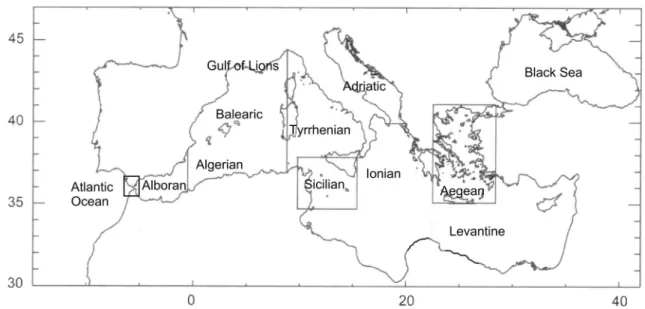
The Mediterranean Sea is a semi-enclosed basin confined between Southern Europe, the Middle East and Northern Africa, only connected to the global ocean by the narrow Strait of Gibraltar (Fig. 1). The excess of evaporation over precipitation generates a water deficit in the basin that is compensated by a net inflow of Atlantic Waters (AW) through the Strait (Bethoux and Gentili 1999; Mariotti et al. 2002). These relatively fresher and warmer waters are progressively transformed along their path through the

Electronic supplementary material The online version of this article (https ://doi.org/10.1007/s0038 2-019-05105 -4) contains supplementary material, which is available to authorized users.

* Javier Soto-Navarro jsoto@imedea.uib-csic.es

Extended author information available on the last page of the article

(2)

basin, becoming the Modified Atlantic Waters (MAW), and eventually sinking to intermediate and deep layers in convective processes triggered by winter cooling. The main core of the intermediate waters is produced in winter in the Levantine basin and hence is known as the Levantine Inter- mediate Water (LIW). The LIW recirculates westward at depths between 300 and 500 m towards the Strait of Sicily and finally towards the Strait of Gibraltar, constituting the main thermohaline cell of the basin (Robinson et al. 1991;

Demirov and Pinardi 2002; Waldman et al. 2018). Second- ary cells appear in the spots where the Mediterranean deep waters are produced. In the Eastern basin, these spots are the Adriatic and the Aegean Seas, where strong winter cooling increases the density of the LIW provoking its sinking to the deeper layer and generating the Eastern Mediterranean Deep Water (EMDW) (Roether and Schlitzer 1991; Roether et al.

1996). In the Western Mediterranean, the deep water formation takes place at the Gulf of Lions in winters when strong heat losses through the sea surface are combined with the preconditioning of the surface and intermediate waters, i.e., waters that have previously increase its salinity by different processes in their path along the basin towards the deep water formation area. This facilitates the convection process and the Western Mediterranean Deep Water (WMDW) is generated (Marshall and Schott 1999; Somot et al. 2018a).

This is a very simplified scheme of the so called Mediter- ranean Thermohaline Circulation (MTHC hereinafter), a feature that makes the Mediterranean basin unique, since it is the only mid-latitude marginal sea where deep convective processes typical for the open ocean and high latitudes take place. For this reason, combined with the fact that a rich mesoscale field is present in the basin including a complex current system and structures like filaments and eddies, the

Mediterranean has been described as a miniature laboratory for climate studies (Bethoux et al. 1999).

As a result of MTHC the average residence time of the basin water masses is around 100 years, way shorter than for the global ocean (Malanotte-Rizzoli et al. 2014). In addition, the Mediterranean is one of the most responsive regions to the climate change, and it has been defined as a primary

“hot spot” (Giorgi 2006). Climate change projections point to a warmer and dryer Mediterranean by the end of the twenty-first century, both using global simulations (Giorgi and Lionello 2008; Mariotti et al. 2008; IPCC 2013, 2018), and regional atmosphere simulations (Sanchez-Gomez et al.

2009; Dubois et al. 2012). Due to the complexity of the MTHC and the importance of the mesoscale activity in the basin, to assess how the sea would respond to changes in the atmospheric conditions high resolution ocean climate models are needed (Somot et al. 2008; Li et al. 2012) forced by high resolution atmospheric forcing (Herrmann and Somot 2008) and taking care of the river evolution (Skliris and Lascaratos 2004; Adloff et al. 2015).

In the last decades a strong effort has been carried out to develop and improve regional climatic circulation models for the Mediterranean (Zavatarelli and Mellor 1995; Pinardi and Masetti 2000; Demirov and Pinardi 2002; Fernández et al. 2005; Oddo et al. 2009; Sannino et al. 2009, 2015;

Beuvier et al. 2010, 2012; Escudier et al. 2016; Hamon et al. 2016; Waldman et al. 2017; Somot et al. 2018a). In the recent years, the skills of the models to reproduce complex processes as the basin mesoscale dynamics (Escudier et al.

2016), the Eastern Mediterranean Transient (EMT) (Beuvier et al. 2010), the deep water formation in the Gulf of Lions (Somot et al. 2018a) or the exchange through the Strait of Gibraltar (Soto-Navarro et al. 2015) have been satisfactorily

Fig. 1 Map of the Mediterranean Sea basin and sub-basins

(3)

tested. Indeed, the regional models have been proven as a very useful tool to reproduce and understand many aspects of the present Mediterranean climate that would have been impossible to study from an observational perspective or using global low resolution models.

However, up to now only a few works have dealt with the investigation of future climate projections at regional scale.

Thorpe and Bigg (2000) studied the future evolution of the Mediterranean waters outflowing to the Atlantic through the Strait of Gibraltar, finding a reduction in the deep water production of the basin. Somot et al. (2006) performed the first realistic scenario simulation (SRES-A2), projecting a general warming and salinity increase of the whole water column in the basin (+ 3.1 °C and + 0.48 psu for the surface and + 1.5 °C and + 0.23 psu for the deep layer), and a reduction of − 40% in the intensity of the MTHC. The future changes in the heat and freshwater budgets were addressed by Sanchez-Gomez et al. (2009) and Dubois et al.

(2012) using A1B scenario simulations for the first half of the twenty-first century. Both works agree in expecting an increase of the freshwater deficit and the heat content of the basin by the year 2050. Gualdi et al. (2013), using the same ensemble of coupled simulations, confirmed the previous results and estimated a sea surface warming between + 1.5 and + 2 °C by 2050 under the A1B scenario. A more recent work of Adloff et al. (2015), based on an ensemble of five simulations based on NEMOMED8 model run under three scenarios (A1B, A2 and B1) and using different boundary conditions, found a warming ranging between + 1.73 and + 2.97 °C and a change in the salinity between + 0.48 and + 0.89 psu by 2100. The authors conclude that the choice of scenario is the most important element conditioning the warming while the boundary conditions in the Atlantic are more decisive in the evolution of the salinity and the Medi- terranean water masses. Macias et al. (2015) studied the projected evolution of primary productivity in the Mediter- ranean using four simulations ran under RCP 4.5 and RCP 8.5 scenarios. Their results did not show significant net changes at basin scale but showed important variations in the spatial distribution of the productivity areas. The same ensemble of simulations was used by Macias et al. (2018) to study the biochemical response of the Mediterranean to the changes in the freshwater budget. The results showed a high sensitivity of the sea surface salinity to the evolution of the freshwater budget, which evolution is very dependent on the choice of scenario.

The previous works listed were based on a single simulation (Thorpe and Bigg 2000; Somot et al. 2006), an ensemble of 5 multi-model simulations using a single scenario and covering only the first half of the twenty-first century (Gualdi et al. 2013) or an ensemble of multi-scenario simulations using the same model (Adloff et al. 2015; Macias et al. 2015, 2018). Recently, and thanks to the efforts of

the different institutions contributing to the Med-COR- DEX initiative (https ://www.medco rdex.eu/; Ruti et al.

2015), coordinated multi-model and multi-scenario studies of the Mediterranean are possible. For example, very recently, Darmaraki et al. (2019) analyzed the evolution of sea surface temperature and marine heat waves (MHW) in the twenty-first century using an ensemble of 17 fully coupled atmosphere–ocean simulations. The ensemble projects stronger and more intense MHW in the future, as a result of the increase of the mean SST. The authors also concluded that the choice of emission scenario became more determin- ing for the MHW characteristics by the second half of the twenty-first century.

In this work we extend and complement previous studies using the Med-CORDEX ensemble to assess the future evolution of the Mediterranean water properties in the whole water column. For the first time, an ensemble of 25 simulations based on six different regional climate models and run under three different emission scenarios has been gathered and analyzed. Our objective is twofold: first, to evaluate the response of the water properties of the Mediterranean Sea under different scenarios of global warming and based on the largest simulation ensemble available until now. Second, to analyze the sensitivity of the projections to the different configurations of the simulations: emission scenario, regional climate model and global model used. The paper is organized as follows: in Sect. 2 the main characteristics of models and simulations are described and the results of the validation for the present climate are analyzed. In Sects. 3 and 4, the results for the temperature and heat budget and for the salinity and salt budget are presented, respectively.

In Sect. 5 we study the evolution the main Mediterranean water masses and the deep convection processes. Finally, the discussion of the results and the main conclusions are presented in Sects. 6 and 7.

2 Models and simulations

2.1 Description of models and simulations

Simulations from six different Regional Climate Models (RCM) provided by six research institutions member of the Med-CORDEX initiative have been analyzed in this study.

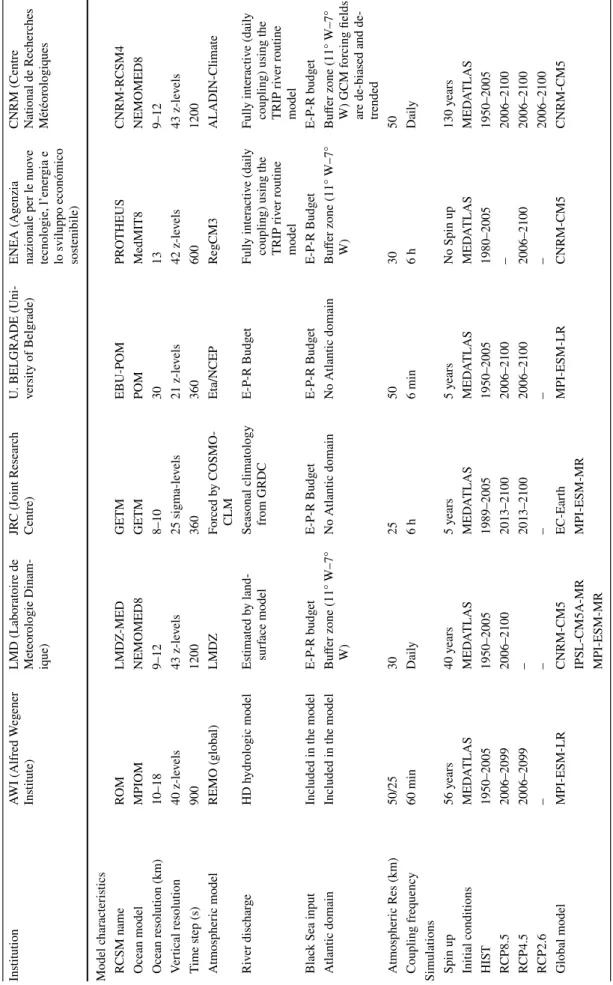
The main characteristics of models and simulations are summarized in Table 1 and described in detail in the supplementary material (SM), so here only the main aspects are presented. Five of the RCM are coupled ocean–atmosphere regional climate system models (RCSM) (ROM from AWI, LMDZ-MED from LMD, EBU-POM from UBEL, PRO- THEUS from ENEA and CNRM-RCSM4 from CNRM) and one is forced (GETM from JRC). Hereinafter each model will be identified by the name of the institution that provides

(4)

Table 1 Summary of the main characteristics of the Med-CORDEX ensemble used in this study InstitutionAWI (Alfred Wegener Institute)LMD (Laboratoire de Meteorologie Dinam- ique)

JRC (Joint Research Centre)U. BELGRADE (Uni- versity of Belgrade)ENEA (Agenzia nazionale per le nuove tecnologie, l’energia e

lo sviluppo económico sostenibile)

CNRM (Centre National de Recherches Météorologiques Model characteristics RCSM nameROMLMDZ-MEDGETMEBU-POMPROTHEUSCNRM-RCSM4 Ocean modelMPIOMNEMOMED8GETMPOMMedMIT8NEMOMED8 Ocean resolution (km)10–189–128–1030139–12 Vertical resolution40 z-levels43 z-levels25 sigma-levels21 z-levels42 z-levels43 z-levels Time step (s)90012003603606001200 Atmospheric modelREMO (global)LMDZForced by COSMO- CLMEta/NCEPRegCM3ALADIN-Climate River dischargeHD hydrologic modelEstimated by land- surface modelSeasonal climatology from GRDCE-P-R BudgetFully interactive (daily coupling) using the TRIP river routine model

Fully interactive (daily coupling) using the TRIP river routine model Black Sea inputIncluded in the modelE-P-R budgetE-P-R BudgetE-P-R BudgetE-P-R BudgetE-P-R budget Atlantic domainIncluded in the model

Buffer zone (11° W–7° W)

No Atlantic domainNo Atlantic domain

Buffer zone (11° W–7° W) Buffer zone (11° W–7° W) GCM f

orcing fields are de-biased and detrended Atmospheric Res (km)50/253025503050 Coupling frequency60 minDaily6 h6 min6 hDaily Simulations Spin up56 years40 years5 years5 yearsNo Spin up130 years Initial conditionsMEDATLASMEDATLASMEDATLASMEDATLASMEDATLASMEDATLAS HIST1950–20051950–20051989–20051950–20051980–20051950–2005 RCP8.52006–20992006–21002013–21002006–2100–2006–2100 RCP4.52006–2099–2013–21002006–21002006–21002006–2100 RCP2.6–––––2006–2100 Global modelMPI-ESM-LRCNRM-CM5EC-EarthMPI-ESM-LRCNRM-CM5CNRM-CM5 IPSL-CM5A-MRMPI-ESM-MR MPI-ESM-MR

(5)

it. The resolution of the ocean models ranges between 8 and 30 km (eddy-resolving), and between 25 and 50 km for the atmospheric models. The domains cover the Mediterranean region and a small part of the Atlantic close to the Strait of Gibraltar (except JRC, that don’t have Atlantic Domain and AWI that includes a large domain in the Atlantic). The contribution of rivers is explicitly modeled by a hydrologic component in all the models except JRC, which keeps river runoff constant. The Black Sea input is parameterized from the freshwater budget in the Black Sea with the exception of AWI which explicitly solves it.

The ensemble is comprised by a total of 25 simulations:

10 historical runs and 15 twenty-first century projections.

The lateral boundary conditions for the atmospheric and ocean components are provided by 5 different Global Cli- mate Models (GCMs). All the projections are run under the Radiative Concentration Pathway (RCP) socio – economic scenarios (Meinshausen et al. 2011). Among them, two main emission scenarios are considered: RCP 8.5 (9 simulations) and RCP 4.5 (5 simulations). Only one simulation has been run under the most optimistic RCP 2.6 scenario, the clos- est to the Paris agreement targets. Taking into account the large number of simulations that are being analyzed, it is important to clarify the criteria used for their identification along the text. Each simulation is noted by three elements:

RCM institution name, GCM name and RCP scenario.

Additionally, AWI simulations include the resolution of the atmospheric model in the institution name. Therefore, AWI50-MPI-8.5 is the simulation run by AWI, with 50 km atmospheric resolution, using the MPI GCM and under RCP8.5 scenario. When the results discussed concern a fam- ily of simulations (i.e., all the simulations run by the same institution) they will be noted using only the institution name (AWIs, LMDs, JRCs, or CNRMs). The specific details of each simulation are summarized in Table 1.

2.2 Present climate validation

Before starting the analysis of the projections and to cor- rectly understand their range of accuracy it is necessary to assess the ability of the models to reproduce the ocean climate statistics during the past decades. In particular we focus on the SST and SSS, as well as on the deeper thermohaline properties of the Mediterranean waters. Considering that, by construction, the simulations cannot be expected to follow the chronology of past atmospheric states (i.e.: no data assimilation is involved), we evaluate their mean state and the spatio-temporal characteristics of the variability. In particular we analyze the amplitude of the seasonal cycle, the magnitude of the interannual variability and the trends of temperature and salinity at the surface (0–150 m), intermediate (150–600 m) and deep (600 m—bottom) layers. The goal of this evaluation is to characterize the model behavior in

Table 1 (continued) InstitutionAWI (Alfred Wegener Institute)LMD (Laboratoire de Meteorologie Dinam- ique)

JRC (Joint Research Centre)U. BELGRADE (Uni- versity of Belgrade)ENEA (Agenzia nazionale per le nuove tecnologie, l’energia e

lo sviluppo económico sostenibile)

CNRM (Centre National de Recherches Météorologiques Short names: Institution + Atms. Res. (if needed) + GCM + RCP(HIST)

AWI50-MPI-HISTLMD-CNRM-HISTJRC-EC-HISTUBEL-MPI-HISTENEA-CNRM-HISTCNRM-CNRM-HIST AWI25-MPI-HISTLMD-IPSL-HISTJRC-MPI-HISTUBEL-MPI-8.5ENEA-CNRM-4.5CNRM-CNRM-8.5 AWI50-MPI-8.5LMD-ESM-HISTJRC-EC-8.5CNRM-CNRM-4.5 AWI50-MPI-4.5LMD-CNRM-8.5JRC-EC-4.5CNRM-CNRM-2.6 AWI25-MPI-8.5LMD-IPSL-8.5JRC-MPI-8.5 LMD-ESM-8.5JRC-MPI-4.5 ReferencesSein et al. (2015)L’Hévéder et al. (2013)Macías et al. (2018)Djordjevic and Raijko- vic (2010)Artale et al (2010)Sevault et al. (2014)

(6)

order to evaluate their accuracy in the representation of the future climate. In the case of the trend analysis, more than to evaluate climatic signals, the objective is to identify if there are any simulation showing anomalous drifts. The detailed explanation of the models drifts or bias is out of the scope of this study. More exhaustive validation of the different simulations can be found in the references cited in Table 1.

It is worth to point out that historical and control runs are only available after 1950 because the GCM files required to force the RCMs were not stored at the CMIP5 database.

For the evaluation, we use as reference two state-of-the- art reanalysis products: one based on dynamical interpolation from the Copernicus Marine Environment Monitor- ing Service (CMEMS; https ://www.marin e.coper nicus .eu) (Simoncelli et al. 2014) and another based on statistical interpolation (MEDHYMAP2.2) (Jordà et al. 2017). The historical runs have been compared with the reference products over their common periods (1987–2005). The average results of the whole basin are outlined in Tables 2 and 3.

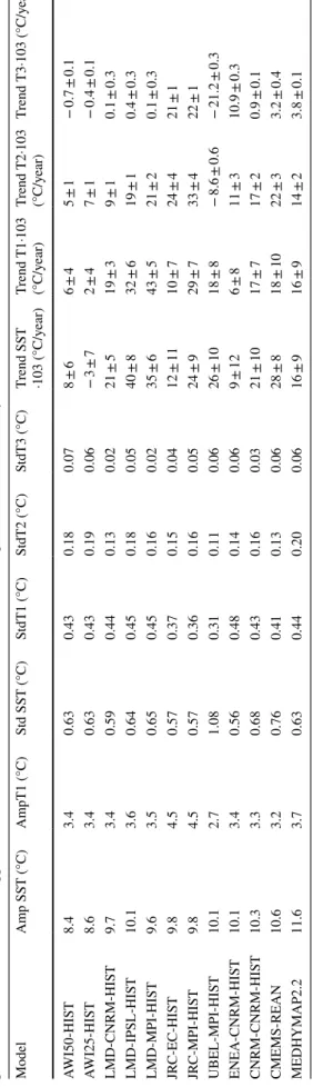
First we analyze the seasonal cycle, which is a good indica- tor of the skills of the models reproducing air-sea interac- tions (for the temperature), and the circulation patterns in the upper layer (for the salinity). For the amplitude of the seasonal cycle, only the surface and upper layers have been considered because no significant seasonality is observed in the deeper layers. The SST seasonal amplitudes of the reanalyses are 10.6 °C in CMEMS-REAN and 11.6 °C in MEDHYMAP2.2. All the simulations show smaller amplitudes, between 8.4 °C (AWI50-HIST) and 10.3 (CNRM- HIST) (Table 2). This bias is somehow corrected when the first 150 m are considered. In the upper layer most of the simulations show amplitudes ranging from 3.3 to 3.6 °C, very close to those of the reanalysis (3.7 °C for CMEMS- REAN and 3.2 °C for MEDHYMAP2.2), only JRCs simulations (4.5 °C) and UBEL-MPI-HIST (2.7 °C) are out from the observed range. For the SSS, the seasonal cycle amplitudes of the reanalyses are 0.51 psu for CMEMS-REAN and 0.42 psu for MEDHYMAP2.2 (Table 3). AWIs, UBEL-MPI- HIST and JRC-EC-HIST simulations show smaller amplitudes (0.22, 0.27 and 0.38 psu, respectively), while in LMDs and CNRM-CNRM-HIST simulations the amplitudes are higher (between 0.67 and 0.84 psu). Only JRC-MPI-HIST (0.41 psu) and ENEA-CNRM-HIST (0.45 psu) show SSS amplitudes similar to those of the reanalyses. As for the temperature, when the whole upper layer is considered the bias is reduced. All the simulations show an amplitude of the seasonal cycle within the range of the reanalyses (0.15–0.24 psu), with the exception of UBEL-MPI HIST which has an amplitude of 0.10 psu. The phase of the cycle agrees well in models and reanalyses, with maximum in September and July for T and S respectively and minimum in March for both variables in the surface and upper layers (not shown).

Table 2 Models validation. Basin mean seasonal cycle amplitude (Amp), standard deviation of the detrended annual time series (Std) (proxy to the interannual variability) and trends of the temperature (T) at the surface (SST), upper (1) (0–150 m), intermediate (2) (150–600 m) and deep (3) (600 m—bottom) layers The trends are computed for the last 25 years of the historical simulations and the error intervals are estimated at 95% confidence level

ModelAmp SST (°C)AmpT1 (°C)Std SST (°C)StdT1 (°C)StdT2 (°C)StdT3 (°C)Trend SST ·103 (°C/year)Trend T1·103 (°C/year)Trend T2·103 (°C/year)Trend T3·103 (°C/year) AWI50-HIST8.43.40.630.430.180.078 ± 66 ± 45 ± 1− 0.7 ± 0.1 AWI25-HIST8.63.40.630.430.190.06− 3 ± 72 ± 47 ± 1− 0.4 ± 0.1 LMD-CNRM-HIST9.73.40.590.440.130.0221 ± 519 ± 39 ± 10.1 ± 0.3 LMD-IPSL-HIST10.13.60.640.450.180.0540 ± 832 ± 619 ± 10.4 ± 0.3 LMD-MPI-HIST9.63.50.650.450.160.0235 ± 643 ± 521 ± 20.1 ± 0.3 JRC-EC-HIST9.84.50.570.370.150.0412 ± 1110 ± 724 ± 421 ± 1 JRC-MPI-HIST9.84.50.570.360.160.0524 ± 929 ± 733 ± 422 ± 1 UBEL-MPI-HIST10.12.71.080.310.110.0626 ± 1018 ± 8− 8.6 ± 0.6− 21.2 ± 0.3 ENEA-CNRM-HIST10.13.40.560.480.140.069 ± 126 ± 811 ± 310.9 ± 0.3 CNRM-CNRM-HIST10.33.30.680.430.160.0321 ± 1017 ± 717 ± 20.9 ± 0.1 CMEMS-REAN10.63.20.760.410.130.0628 ± 818 ± 1022 ± 33.2 ± 0.4 MEDHYMAP2.211.63.70.630.440.200.0616 ± 916 ± 914 ± 23.8 ± 0.1

(7)

The magnitude of the interannual variability has been quantified using the standard deviation of the detrended annual anomalies. The SST variability is slightly smaller than the reanalysis data (0.76 °C in CMEMS-REAM and 0.63 °C in MEDHYMAP2.2) in JRCs (0.57 °C), ENEA- CNRM-HIST (0.56 °C) and LMD-CNRM-HIST (0.59 °C) simulations (Table 2). For UBEL-MPI-HIST the variability is very high (1.08 °C), while the rest of the simulations are in the range of the reanalyses. In the upper and intermediate layers, simulation and reanalyses show similar values (Table 2). In the first 150 m most simulations show values close to the observations (0.41–0.44 °C). JRCs SST have slightly smaller variability (0.36–0.37 °C) and UBEL-MPI- HIST simulation is the one showing the largest discrepancy (0.31 °C). It is interesting to note that this simulation has a strong positive bias in the SST that is drastically reduced when the whole upper layer is considered. For the intermediate layer all the simulations fall in the reanalyses range (0.13–0.20 °C) except the UBEL-MPI-HIST run (0.11 °C). In the deeper layer, the reanalyses have the same value 0.06 °C, LMD-CNMR-HIST, LMD-MPI-HIST and CNRM-CNRM-HIST simulations show a smaller variability (0.02–0.03 °C) while for the rest the values are very close to both reanalyses.

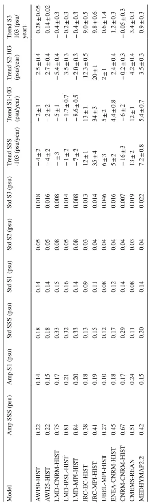
The standard deviation of the interannual variability of the SSS in the reanalyses is 0.11 psu for CMEMS-REAN and 0.20 for MEDHYMAP2.2. All the simulations have values within this range, except LMDs which show higher standard deviation values (0.32–0.33 °C) (Table 3). In the first two layers of the water column, the salinity interannual variability does not show very significant discrepancies between simulations and reanalyses. In the upper layer the variability ranges between 0.08 and 0.14 psu in the reanalyses while ranging between 0.08 and 0.16 psu in the models.

In the intermediate layer, all simulations oscillate between 0.03 and 0.05, in good agreement with the reanalyses, except for LMD-CNRM-HIST and LMD-MPI-HIST, both with values of 0.08 psu. Higher differences are found in the deepest layer, where the values for CMEMS and MEDHYMAP are 0.022 and 0.019 psu respectively while for some simulations (LMD-CNRM-HIST, LMD-MPI-HIST and CNRM-CNRM- HIST) standard deviation values are one order of magnitude lower (0.008 psu) and for UBEL-MPI-HIST is more than double (0.046 psu) the standard deviation of the reanalyses.

Finally, we assess the temperature and salinity trends. It has to be noted that decadal variations may affect the 25-year trend estimates. As the historical simulations are not con- straint to follow the observed chronology, we cannot expect a perfect match between reanalysed and modeled 25-year trends, especially in the upper layer where the decadal variations are more intense (Macias et al. 2013). Nevertheless, this diagnostic is useful to identify outliers. The basin averaged results are summarized in Tables 2 and 3, and some

Table 3 Same as Table 2 but for salinity (S) ModelAmp SSS (psu)Amp S1 (psu)Std SSS (psu)Std S1 (psu)Std S2 (psu)Std S3 (psu)Trend SSS ·103 (psu/year)Trend S1·103 (psu/year)Trend S2·103 (psu/year)Trend S3 103 (psu/ year)

AWI50-HIST0.220.140.180.140.050.018− 4 ± 2− 2 ± 12.5 ± 0.40.28 ± 0.05 AWI25-HIST0.220.150.180.140.050.016− 4 ± 2− 2 ± 22.7 ± 0.40.14 ± 0.02 LMD-CNRM-HIST0.750.170.330.150.080.008− ± 3− 5 ± 1− 5.4 ± 0.4− 0.4 ± 0.3 LMD-IPSL-HIST0.810.210.320.160.050.014− 1 ± 2− 1.7 ± 0.73.5 ± 0.3− 0.2 ± 0.3 LMD-MPI-HIST0.840.200.330.140.080.008− 7 ± 2− 8.6 ± 0.5− 2.0 ± 0.3− 0.4 ± 0.3 JRC-EC-HIST0.380.180.130.090.030.01312 ± 113 ± 112.3 ± 0.59.0 ± 0.5 JRC-MPI-HIST0.410.190.150.110.040.01435 ± 434 ± 320 ± 19.8 ± 0.6 UBEL-MPI-HIST0.270.100.120.080.040.0466 ± 35 ± 22 ± 10.6 ± 1.4 ENEA-CNRM-HIST0.450.180.170.120.040.0165 ± 24.4 ± 0.82.4 ± 0.41.2 ± 0.3 CNRM-CNRM-HIST0.670.170.290.140.040.007− 16 ± 3− 6 ± 2− 0.2 ± 0.3− 0.05 ± 0.3 CMEMS-REAN0.510.240.110.080.030.01913 ± 212 ± 14.2 ± 0.43.4 ± 0.3 MEDHYMAP2.20.420.150.200.140.040.0227.2 ± 0.85.4 ± 0.73.5 ± 0.30.9 ± 0.3

(8)

discrepancies are clear between simulations and reanalyses.

For the SST the range of trends in the reanalyses (including the uncertainty) is quite large with [7–36] × 10^–3 °C/

year. The only simulation out of this range is AWI25-MPI- HIST, which show a trend of −3 ± 7 × 10⁻³ °C/year. LMD- IPSL-HIST and LMD-MPI-HIST, with 40 ± 8 × 10^–3 °C/

year and 35 ± 6 × 10^–3 °C/year respectively, are in the upper limit of the reanalyses range (Table 2). For the temperature of the upper layer, LMD-CNRM-HIST, JRC-EC- HIST, UBEL-MPI-HIST and CNRM-CNRM-HIST are the only simulations in agreement with the observed range [7–28] × 10^–3 °C/year. The rest show very low (AWI50(25)- MPI-HIST, ENEA-CNRM-HIST simulations) or very high values (LMD-MPI-HIST, LMD-IPSL-HIST, JRC-MPI- HIST simulations) with respect to the observationally-based ones. In the intermediate layer the differences between simulations and reanalyses are not that pronounced, although still quite important for some simulations. In particular for UBEL-MPI-HIST, which is the only simulation with negative trend in this layer (− 8.6 × 10^–3 °C/year) and JRC-MPI- HIST which shows 33 ± 4 × 10^–3 °C/year, well outside the observational range [12–25] × 10^–3 °C/year. In the deep layer the largest discrepancies are found. All simulations show values that are very far from those obtained from the reanalyses [2.8–3.9] × 10^–3 °C/year. AWIs, LMDs and CNRM simulations show very low values, between

− 0.7 × 10^–3 and 0.9 × 10^–3 °C/year while higher trends are shown by ENEA-CNRM-HIST (10 × 10^–3 °C/year) and JRCs (20 × 10^–3 °C/year) simulations. As for the intermediate layer, UBEL-MPI-HIST is the only simulation that shows a highly negative trend (− 21 × 10^–3 °C/year).

The salinity trends show even stronger discrepancies between simulations and reanalyses. For the SSS only JRC-EC-HIST trend is inside the observational range [6.4–15] × 10^–3 psu/year (Table 3). JRC-MPI-HIST has a higher trend and the rest of the simulations show very low or negative values (reaching − 16 × 10^–3 psu/year in CNRM- HIST).In the upper layer both reanalyses product show positive values [4.7–13] × 10^–3 psu/year. AWIs, LMDs and CNRM simulations have negative mean trends ([− 8 to − 2] × 10⁻³psu/

year) while ENEA-CNRM-HIST, UBEL-MPI-HIST and JRCs simulations show positive values, the latter reaching 34 × 10⁻³psu/year. In the intermediate layer the two reanalyses are in better agreement [3.2–4.6] × 10^–3 psu/year. AWIs, LMD-IPSL-HIST, ENEA-CNRM-HIST, and UBEL-MPI- HIST simulations also show positive values of the same order ([2–3.5] × 10⁻³ psu/year). LMD-CNRM-HIST, LMD-MPI- HIST and CNRM-CNRM-HIST simulations have negative trends between − 5.4 × 10⁻³ psu/year and − 0.2 × 10⁻³ psu/

year. JRCs simulations once again show abnormally high trends in this layer reaching 20 × 10⁻³ psu/year. As in the case of the temperature, the largest discrepancies are found in the deepest layer where most models show values outside

the reanalyses range [0.6–3.7] × 10^–3 psu/year. AWIs, LMDs, and CNRM simulations show very low trends, between

− 0.4 × 10⁻³psu/year and 0.3 × 10⁻³psu/year, while in JRCs simulations the trends are once more very high in comparison with the rest of simulations and reanalyses (9–9.8 × 10⁻³psu/

year).

The comparison between models and reanalyses in terms of the spatial patterns of the seasonal cycle amplitude, interannual variability and trends of temperature and salinity is presented in the supplementary material (Figs S1–S14). The results are in the same line than for the basin average, with better agreement between reanalyses and simulations in the upper and intermediate layers, and larger discrepancies in the deep layer. In general, the spatial distribution over the basin of the areas with higher/lower values is satisfactorily reproduced by all the models. However, significant differences are observed for the T and S trends values in the intermediate layer and especially in the deep layer for JRCs, ENEA-CNRM-HIST and UBEL-MPI-HIST simulations.

In summary, in the surface and upper layers, the discrepancies between all the simulations and the reanalyses are in the same range of those obtained in previous works. They are mainly attributed to uncertainties in the surface heat and freshwater fluxes (Nabat et al. 2014; Harzallah et al. 2018; Llasses et al. 2018; Darmaraki et al. 2019). In the intermediate and deep layers, the difficulties of the ocean circulation models to reproduce the salinity and temperature trends have also been reported. Llasses et al. (2018) analyzed 14 hindcast simulations from state-of-the-art ocean models and established that present-day regional models can provide reasonable estimates in the surface and upper layers but below 150 m are less reli- able. In our case, the trends obtained for AWIs, LMDs, and CNRMs for the temperature and also for ENEA-CNRM-HIST for the salinity are in the range of variability of the state-of- the-art models for the Mediterranean. Therefore, the observed biases can be considered a consequence of the models limi- tations. On the contrary, for JRCs, UBEL-MPI-HIST and ENEA-MPI-HIST (only for temperature) the observed drifts are much higher and maintained during the projection. This makes us think that these runs did not reach a stable stationary state in the intermediate and deep layers. For this reason, they will be treated with caution in the analysis of the projections in those layers. They will be identified in figures and tables and excluded from the ensemble average computations.

3 Temperature evolution in the twenty‑first century

3.1 Sea surface temperature

The anomalies of the Sea Surface Temperature (SST), computed as the difference between the last 25 years of

(9)

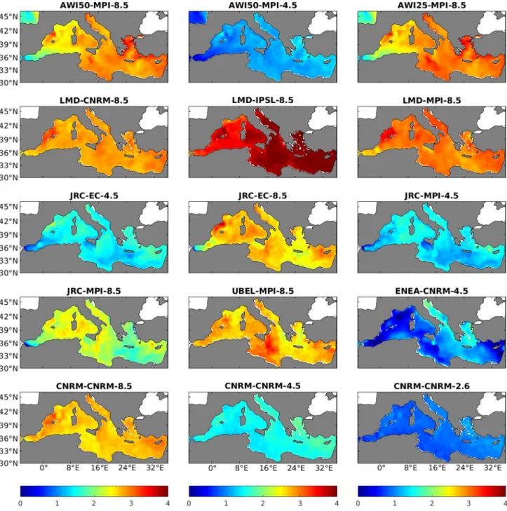
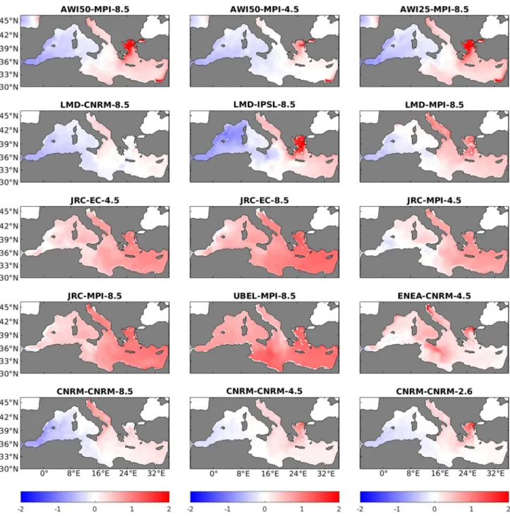
the historical runs (1980–2005) and the last 25 years of the projections (2075–2100), are represented in Fig. 2 and summarized in Table 4 (the periods are 15 years long for JRC). In all the simulations the SST increases by the end of the century but the magnitude and, to a lesser extent, the spatial distribution of this warming significantly varies depending on the simulation. The choice of emissions scenario appears to be the most relevant factor in the vari- ation of the SST by the end of the twenty-first century.

The simulations run under RCP 8.5 scenario show an average increase between 2 and 4 °C, while the simulations run under RCP 4.5 and RCP 2.6 scenarios show lower warming (between 0 and 2 °C). Moreover, if we focus on model configurations that are run under both RCP4.5 and RCP8.5, we find an average increase of 1.30 and 2.43 °C, respectively. The representation of the spatial Root Mean Square Difference (RMSD) between pairs of simulations

Fig. 2 SST anomaly fields (°C) estimated as the difference between the average of the future (2075–2100) and present (1980–2005) conditions.

The corresponding simulation is noted in the title of each panel

(10)

Table 4 3d Temperature anomalies in degrees Celsius (°C) for all the simulations at the surface (SST), upper layer (0–150 m), intermediate layer (150–600 m) and deep layer (600 m–bottom) in the Western (WMED), Eastern (EMED) and whole (MED) basins The last four rows represent the average of the RCP8.5 runs, the average of the RCP4.5 runs and the average of the sub-ensembles of RCP8.5 and RCP4.5 runs performed by the same models (hence suitable for a robust comparison). The outlier simulations in the intermediate and deep layers (see text) are not considered in the computation of the average in the sub-ensembles (UBEL- MPI-8.5 in the intermediate layer; JRCs, UBEL-MPI-8.5 and ENEA-CNRM-4.5 in the deep layer). These simulations are noted with italic fonts. The ensemble and sub-ensemble spreads (± standard deviation) are also included. The anomalies are estimated as the difference between the average of the last 25 years of the twenty-first century (1975–2100) and the last 25 year of the historical run (1980–2005)

ModelSSTUpper layerIntermediate layerDeep layer WMEDEMEDMEDWMEDEMEDMEDWMEDEMEDMED AWI50-MPI-8.52.292.332.802.561.991.991.990.190.160.18 AWI50-MPI-4.50.860.921.091.001.060.931.000.120.130.13 AWI25-MPI-8.52.352.392.882.632.001.981.990.180.150.17 LMD-CNRM-8.52.822.652.772.731.911.741.810.050.020.03 LMD-IPSL-8.53.733.223.973.713.212.832.970.240.090.14 LMD-MPI-8.52.972.682.892.822.362.022.140.080.030.05 JRC-EC-4.51.471.251.511.421.471.791.671.401.731.61 JRC-EC-8.52.642.092.422.302.072.462.321.672.111.95 JRC-MPI-4.51.361.021.151.111.301.691.541.381.761.63 JRC-MPI-8.52.162.052.372.262.022.522.331.451.931.76 UBEL-MPI-8.52.751.802.222.07−0.240.270.07−0.89−0.82−0.84 ENEA-CNRM-4.50.931.211.471.381.341.621.521.391.661.56 CNRM-CNRM-8.52.692.482.542.522.291.781.970.250.140.18 CNRM-CNRM-4.51.521.401.511.471.431.221.300.200.130.15 CNRM-CNRM-2.60.860.750.840.810.860.800.820.180.130.15 Ensemble RCP852.71 ± 0.472.41 ± 0.422.76 ± 0.512.62 ± 0.472.23 ± 0.422.16 ± 0.392.19 ± 0.360.17 ± 0.080.10 ± 0.060.12 ± 0.07 Ensemble RCP451.23 ± 0.311.16 ± 0.191.35 ± 0.211.28 ± 0.211.32 ± 0.161.45 ± 0.361.41 ± 0.270.16 ± 0.050.13 ± 0.010.14 ± 0.02 Sub-Ensemble RCP8.52.42 ± 0.232.24 ± 0.192.53 ± 0.232.41 ± 0.162.09 ± 0.122.19 ± 0.332.15 ± 0.190.21 ± 0.040.15 ± 0.010.18 ± 0.01 Sub-Ensemble RCP4.51.30 ± 0.301.15 ± 0.221.32 ± 0.231.25 ± 0.231.32 ± 0.191.41 ± 0.401.38 ± 0.300.16 ± 0.050.13 ± 0.010.14 ± 0.01

(11)

(Figure S15) allows an easy visualization of the simulations average differences (see SI for details).

The second important element of the simulations setup that determines the average SST evolution is the choice of global model in which the climate model is nested.

For instance, if we focus our attention on the three LMDs simulations, which only differ in the global model they use (Table 1), clear differences can be observed (Fig. 2, Table 4).

The spatial distribution of the warmer and colder areas is similar but the averaged increase of SST in the whole basin is around 3.73 °C in the simulation nested into IPSL-CM5A- MR, a 25% higher than for the one nested to CNRM-CM5 (Fig. S15; Table 4). This effect is also present between the two RCP 8.5 simulations of the JRC: the anomalies in the simulation nested into EC-Earth are 2.64 °C, a ~ 20%

higher than those in the simulation nested into MPI-ESM- LR. Under the RCP 4.5 scenario the differences between the two JRC simulations are smaller (~ 10%), the one using EC- Earth being slightly warmer (Fig. S15, Table 4). The choice of the regional model has also an impact on the averaged warming. Different simulations forced by the same global model MPI under the RCP8.5 shows a warming of 2.16 °C, 2.35 °C and 2.97 °C (for JRC-MPI-8.5, AWI25-MPI-8.5 and LMD-MPI-8.5).

Concerning the spatial structures of the SST anomalies, in general, all simulations show similar features. First, all of them show a rather homogeneous warming across the basin.

Overimposed, there is a longitudinal gradient with higher anomalies towards the Eastern basin. There is also coin- cidence in the location of the regions where the anomalies are especially high, such as the Levantine Basin (concretely in the area surrounding Cyprus), North of the Aegean and Adriatic Seas and the Balearic Sea. However, the specific location, extension and intensity of these warmer areas are not the same for all the simulations. Interestingly, if we check the spatial correlation of SST anomalies among models (see Fig. S16) we find that the simulations based on the same RCM are highly correlated among them. On the other hand, the correlation between runs from different models significantly varies, from very low or even negative values to values higher than 0.6. The choice of the GCM does not have such a noticeable impact in the spatial distribution of the SST. Finally, it is also worth pointing out the very small difference introduced by the increase of resolution in the atmospheric component of the AWIs simulations. AWI25- MPI-8.5 and AWI50-MPI-8.5, with 25 km and 50 km atmospheric resolution respectively, show the same SST spatial patterns, with only a small increase in the anomalies in the former (~ 0.06 °C, Table 1, Fig. 1).

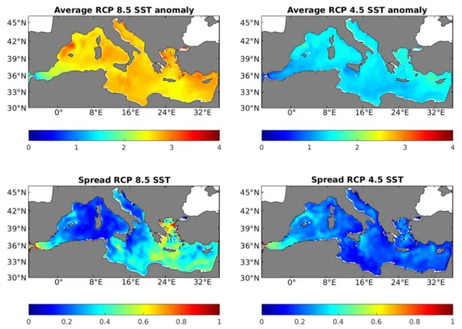
In order to make the comparison of the scenarios more meaningful, we have selected the sub-ensembles of simulations that are run under both RCP8.5 and RCP4.5 scenarios. The results of the averaged SST anomaly for both

sub-ensembles are summarized in Fig. 3. The ensemble of RCP8.5 runs show an increase between 1.5 and 2 °C, higher than the ensemble of RCP4.5 runs. These differences are quite homogeneous over the basin. They are slightly lower in the Adriatic and the Aegean Seas (~ 1.5 °C), and slightly higher in the Northwestern Mediterranean, the Ion- ian Sea and the Levantine basin (~ 2 °C). The regional differences among models described before are reflected into the ensemble spread (standard deviation). For the RCP8.5 runs the higher discrepancies among models (0.6–0.9 °C) are found in the Strait of Gibraltar area, and wide areas in the Levantine basin, the Aegean and the Ionia Seas. In the RCP4.5 ensemble the spread is generally lower, with higher values (~ 0.6 °C) in the Alboran Sea and the Northwestern Mediterranean.

3.2 3D temperature

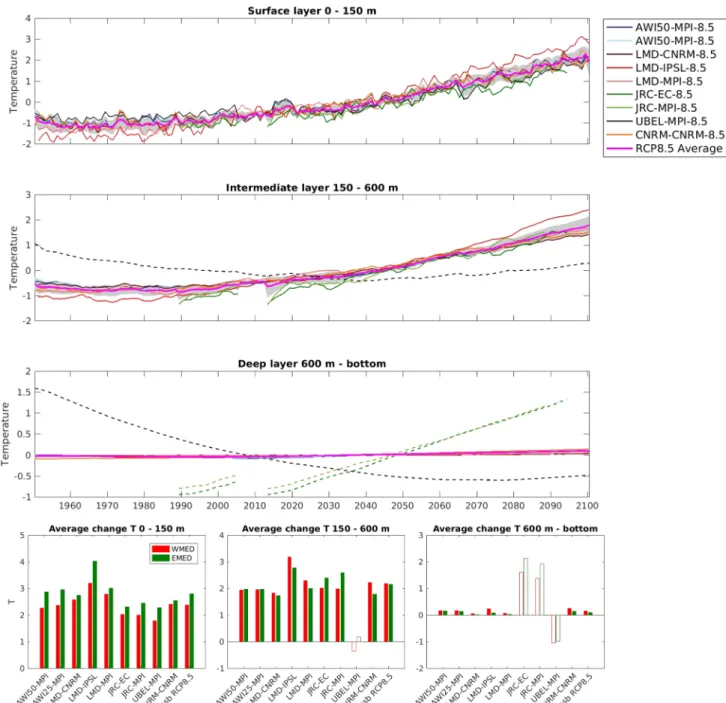
The time series of anomalies of temperature for the surface, intermediate and deep layers are represented in Fig. 4 (for clarity only the RCP 8.5 simulations are included in the figure). Table 4 summarizes the temperature anomalies for all simulations distributed by layers and basins.

The dashed lines and discolored bars in Fig. 4 indicate the simulations that showed anomalous drifts in the intermediate and deep layers in the historical runs. These runs have not been included in the computation of the ensemble anomalies of Table 4 (noted with italic fonts) (UBEL- MPI-8.5 in the intermediate layer; JRCs, UBEL-MPI-8.5 and ENEA-CNRM-4.5 in the deep layer). In the upper layer, all the simulations show an increase of temperature in both sub-basins but higher in the Eastern one in all cases. This increase (for the whole basin) among the RCP8.5 scenario runs ranges between 3.7 °C for LMD-CNRM-8.5 simulation and 2.0 °C for UBEL-MPI-8.5. For the RCP4.5 runs the maximum warming is 1.4 °C for CNRM-CNRM-4.5 simulation and the minimum 1 °C for AWI50-MPI-4.5. Under the RCP2.6 scenario only one simulation is available (CNRM- CNRM-2.6) which shows an averaged warming of 0.84 °C at the end of the century (Table 4). The results are in good agreement with the results presented above for the SST. The simulations that showed higher SST anomalies are the ones projecting higher warming in the surface layer, with strong dependence on the scenario and the global models they use.

In the intermediate layer a substantial temperature increase is also projected by most simulations ranging from 1.1 to 2.9 °C. Larger/smaller changes are projected by those models which also project larger/smaller changes in the upper layer (Fig. 4). In this layer the warming of the West- ern and Eastern basins is very similar in most models and consequently in the ensemble mean. The outlier is UBEL- MPI-8.5, which shows a slightly warming in the Eastern basin (0.2 °C) and even a slightly cooling in the WMED

(12)

(− 0.2 °C), as a consequence of the above mentioned drift.

For the entire basin, the ensemble average shows a warming in the intermediate layer of 2.16 °C under the RCP8.5 scenario. When only the sub-ensemble run under both scenarios is considered the warming is 2.15 °C for the RCP8.5 scenario and 1.38 °C for the RCP4.5 scenario.

In the deep layer the runs with strong temperature drifts in the historical period introduce a very significant bias in the ensemble-mean statistics. UBEL-MPI-8.5 has strong negative anomalies, while JRCs and ENEA-CNRM-4.5 have very high positive anomalies (Table 4). The projected change in these simulations is one order of magnitude larger than for some of the runs of the rest of the ensemble. The drift is very clear in the time series representation of Fig. 4 (dashed lines for JRCs, and UBEL-MPI-8.5; note that the y-axis scale in the panel has been widen to highlight the strong differences between drifting and non-drifting simulations). When excluding them from the ensemble average computation, the projected change of temperature for the whole basin in the deepest layer is 0.12 °C under the RCP8.5 scenario, and 0.14 °C under RCP4.5.

3.3 Heat budget evolution

In order to understand the mechanisms responsible of the warming described in the previous section the heat budget has been analyzed, separating the contributions of the surface heat flux and the heat exchange through the Strait of Gibraltar.

The temporal evolution of the basin heat content is approximated by the equations:

The left hand side of Eq. 1 is the temporal derivative of the basin heat content (HC) that is equal to the sum of the heat flux at the sea surface (Q_Surf) and the heat exchanged through Gibraltar (QGib). In Eq. 2, developing the term on the left hand side of Eq. 1, we have the water specific heat, C_p, the basin volume, V, the water density, ρ, and the time derivative of the basin temperature, dT/dt. On the second term of the right hand side we have simplified the Gibraltar dHC_Med (1)

dt =Q_Surf +Q_Gib

(2) CpV𝜌dT

dt =Q_Surf+Cp𝜌(G_inT_Gin−G_outT_Gout)

Fig. 3 Average SST anomalies (°C) for the RCP 8.5 runs (top left) and RCP 4.5 runs (top right). The bottom left and right panels are the spread of the RCP 8.5 and RCP 4.5 sub-ensembles, respectively

(13)

exchange as a two layer exchange (Soto-Navarro et al. 2010), so G_in(out) and T_in(out) are the volume transport of the inflow (outflow) and the inflow (outflow) temperature respectively.

It is worth mentioning that the inflow is composed by Atlan- tic waters while the outflow is mainly composed by Mediter- ranean intermediate waters.

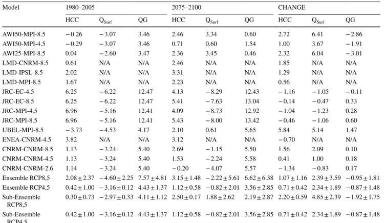
The averaged values for the end of the historical runs (1980–2005) and for the end of the twenty-first century projections (2075–2100) of the heat content change (HCC), the surface heat flux (Q_Surf) and the heat flux through the Strait of Gibraltar (QG) are summarized in Table 5. It is important to point out that the closure of the heat budget is not always achieved due to the use of monthly data in the computation.

Fig. 4 Time series of the basin 3d averaged temperature (°C) at the upper (0–150 m, top panel), intermediate (150–600 m, middle panel) and deep (600 m–bottom, bottom panel) layers for the RCP 8.5 simulations. The magenta thick line is the ensemble mean and the shaded area represents the ensemble standard deviation. The bars in the bottom row represent the average temperature anomalies between the

future (2075–2100) and the present (1980–2005) at each layer for the Western (red) and Eastern (green) basins for each model. Note the different vertical axis. The dashed lines and discolored bars indicate the simulations with anomalous drifts (see text). These simulations are not considered in the computation of the ensemble average