CHEMICAL SPECIATION OF ENVIRONMENTALLYSIGNIFICANT HEAVY METALS WITH INORGANICLIGANDSPART 1:THE Hg

DOI: 10.1351/pac200577040739

© 2005 IUPAC

INTERNATIONAL UNION OF PURE AND APPLIED CHEMISTRY ANALYTICAL CHEMISTRY DIVISION*

CHEMICAL SPECIATION OF ENVIRONMENTALLY SIGNIFICANT HEAVY METALS WITH INORGANIC

LIGANDS

PART 1: THE Hg ²⁺ – Cl ^– , OH ^– , CO ₃ ^2– , SO ₄ ^2– , AND PO ₄ ^3– AQUEOUS SYSTEMS

(IUPAC Technical Report)

Prepared for publication by

KIPTON J. POWELL^1,‡, PAUL L. BROWN², ROBERT H. BYRNE³, TAMÁS GAJDA⁴, GLENN HEFTER⁵, STAFFAN SJÖBERG⁶, AND HANS WANNER⁷

1Department of Chemistry, University of Canterbury, Christchurch, New Zealand; ²Australian Sustainable Industry Research Centre, Building 4W, Monash University, Gippsland Campus, Churchill VIC 3842, Australia; ³College of Marine Science, University of South Florida, 140 Seventh

Avenue South, St. Petersburg, FL 33701-5016, USA; ⁴Department of Inorganic and Analytical Chemistry, University of Szeged, P.O. Box 440, Szeged 6701, Hungary; ⁵School of Mathematical and

Physical Sciences, Murdoch University, Murdoch, WA 6150, Australia; ⁶Department of Inorganic Chemistry, Umeå University, S-901 87 Umeå, Sweden; ⁷Swiss Federal Nuclear Safety Inspectorate,

CH-5232 Villigen, Switzerland

*Membership of the Analytical Chemistry Division during the final preparation of this report:

President: K. J. Powell (New Zealand); Titular Members: D. Moore (USA); R. Lobinski (France); R. M. Smith (UK); M. Bonardi (Italy); A. Fajgelj (Slovenia); B. Hibbert (Australia); J.-Å. Jönsson (Sweden); K. Matsumoto (Japan); E. A. G. Zagatto (Brazil); Associate Members: Z. Chai (China); H. Gamsjäger (Austria); D. W. Kutner (Poland); K. Murray (USA); Y. Umezawa (Japan); Y. Vlasov (Russia); National Representatives: J. Arunachalam (India); C. Balarew (Bulgaria); D. A. Batistoni (Argentina); K. Danzer (Germany); W. Lund (Norway); Z. Mester (Canada); Provisional Member: N. Torto (Botswana).

‡Corresponding author

Republication or reproduction of this report or its storage and/or dissemination by electronic means is permitted without the need for formal IUPAC permission on condition that an acknowledgment, with full reference to the source, along with use of the copyright symbol ©, the name IUPAC, and the year of publication, are prominently visible. Publication of a translation into another language is subject to the additional condition of prior approval from the relevant IUPAC National Adhering Organization.

Chemical speciation of environmentally significant heavy metals with inorganic ligands. Part 1: The Hg ²⁺ – Cl ^– , OH ^– , CO ₃ ^2– , SO ₄ ^2– , and PO ₄ ^3– aqueous systems

(IUPAC Technical Report)

Abstract: This document presents a critical evaluation of the equilibrium constants and reaction enthalpies for the complex formation reactions between aqueous Hg(II) and the common environmental inorganic ligands Cl^–, OH^–, CO₃^2–, SO₄^2–, and PO₄^3–. The analysis used data from the IUPAC Stability Constants database, SC-Database, focusing particularly on values for 25 °C and perchlorate media.

Specific ion interaction theory (SIT) was applied to reliable data available for the ionic strength range I_c≤3.0 mol dm^–3.

Recommended values of log₁₀β_p,q,r° and the associated reaction enthalpies,

∆_rH_m°, valid at I_m= 0 mol kg^–1and 25 °C, were obtained by weighted linear re- gression using the SIT equations. Also reported are the equations and specific ion interaction coefficients required to calculate log₁₀ β_p,q,r values at higher ionic strengths and other temperatures. A similar analysis is reported for the reactions of H⁺with CO₃^2–and PO₄^3–.

Diagrams are presented to show the calculated distribution of Hg(II) amongst these inorganic ligands in model natural waters. Under typical environ- mental conditions, Hg(II) speciation is dominated by the formation of HgCl₂(aq), Hg(OH)Cl(aq), and Hg(OH)₂(aq).

Keywords: chemical speciation; heavy metals; environmental; ligands; stability constants; Division V.

CONTENTS

1. INTRODUCTION 2. OBJECTIVES

3. SUMMARY OF RECOMMENDED VALUES

4. Hg(II) SOLUTION CHEMISTRY 5. DATA EVALUATION METHODS

5.1 Data evaluation criteria

5.2 Methods for numerical extrapolation of data to I_m= 0 mol kg^–1 5.3 Criteria for the assignments: “Recommended” and “Provisional”

6. EVALUATION OF EQUILIBRIUM CONSTANTS (HOMOGENEOUS REACTIONS) 6.1 The Hg²⁺– OH^–system

6.1.1 Formation of HgOH⁺ 6.1.2 Formation of Hg(OH)₂(aq)

6.1.3 Formation of Hg(OH)₃^–, Hg₂OH³⁺, and Hg₂(OH)₂²⁺

6.2 The Hg²⁺– Cl^–system 6.2.1 Formation of HgCl⁺ 6.2.2 Formation of HgCl₂(aq)

6.2.3 Formation of HgCl₃^–and HgCl₄^2–

6.2.4 Other binary Hg(II) chloro complexes

6.3 The Hg²⁺– OH^–– Cl^–system: Formation of HgOHCl(aq) 6.4 The Hg²⁺– CO₃^2–system

6.5 The Hg²⁺– PO₄^3–system 6.6 The Hg²⁺– SO₄^2–system

7. SPECIATION IN 2-COMPONENT SYSTEM: H⁺– L 7.1 The H⁺– CO₃^2–system

7.2 The H⁺– PO₄^3–system

8. EVALUATION OF EQUILIBRIUM CONSTANTS FOR HETEROGENEOUS REACTIONS 8.1 The Hg²⁺– OH^–system: Solubility of HgO(s)

8.2 The Hg²⁺– Cl^–system: Solubility of HgCl₂(s)

8.3 The Hg²⁺– CO₃^2–system: Solubility of HgCO₃2HgO(s) 8.4 The Hg²⁺– PO₄^3–system

9. EVALUATION OF ENTHALPY DATA (HOMOGENEOUS AND HETEROGENEOUS RE- ACTIONS)

9.1 The Hg²⁺– OH^–system 9.2 The Hg²⁺– Cl^–system

10. SPECIATION IN MULTICOMPONENT SYSTEMS: Hg²⁺– H⁺– Cl^–– CO₃^2–– PO₄^3–– SO₄^2–

10.1 Freshwater in equilibrium with CO₂(g)

10.2 Freshwater with varying chloride concentrations 10.3 Summary

REFERENCES APPENDIX 1A

Stability constants and equilibrium constants Nomenclature for stability constants

APPENDIX 1B

Complex formation by polyvalent anions (SO₄^2–, PO₄^3–, CO₃^2–) APPENDIX 2

Selected equilibrium constants APPENDIX 3

SIT plots for Hg²⁺– L systems APPENDIX 4

Equilibrium data for the systems H⁺– CO₃^2–and H⁺– PO₄^3–

1. INTRODUCTION

This review is the first in a series relevant to speciation of heavy metal ions in environmental systems of low ionic strength. The series will provide access to the best possible equilibrium data for chemical speciation modeling of reactions of heavy metal ions with the major inorganic ligands. The metal ions and ligands selected for review are: Hg²⁺, Cd²⁺, Cu²⁺, Pb²⁺, Zn²⁺and Cl^–, OH^–, CO₃^2–, SO₄^2–and PO₄^3–, respectively. To enable speciation calculations on these systems, recommended values for the H⁺– CO₃^2–and –PO₄^3–systems are also reported.

Chemical speciation modeling for labile systems is based on the assumption that all component and derived species are in equilibrium and that reliable stability constants are available at the applica- ble ionic strength and temperature. The validity of these assumptions is often uncertain. Further, full de- tails of component (stoichiometric) concentrations are required. Despite these factors, modeling has definite value in interpretation or simulation of environmental processes. It is often the only option as the necessary sensitive, selective, and noninvasive analytical techniques for measuring metal ion and metal complex concentrations are still, to a great extent, unavailable.

Detailed knowledge of chemical speciation is essential to a full understanding of bioavailability and toxicity of heavy metal ions, and to their adsorption, sedimentation, and transport phenomena in soils, rivers, and aquifers. The optimization of many industrial chemical processes, as in hydrometal- lurgy and pulp and paper processing, relies on a detailed understanding of speciation in often-compli- cated multicomponent, multiphase systems.

2. OBJECTIVES

This review is concerned with the Hg²⁺– Cl^–, OH^–, CO₃^2–, SO₄^2–, and PO₄^3–systems. Each review in this series will provide critically evaluated equilibrium data applicable to environmental waters at low ionic strength. Such values are derived from data reported in the IUPAC Stability Constants database, SC-Database [2003PET], and extrapolated to zero ionic strength (I_m= 0 mol kg^–1) using appropriate specific ion interaction theory (SIT) functions [97GRE]. A consequence of this SIT approach, which typically utilized published constants measured at I_c= 0.5–3.0 mol dm^–3, is the generation of empiri- cal functions that permit the calculation of log₁₀K_nvalues at intermediate values of I_mas may be rele- vant in industrial or environmental situations.

For each metal–ligand combination, the review will

• identify the most reliable publications and stability constants;

• identify (and reject) unreliable stability constants;

• establish correlations between the selected data on the basis of ionic strength dependence, using the SIT functions;

• establish recommended values of β_p,q,r° and K_s0at 25 °C (298.15 K) and I_m= 0 mol kg^–1;

• identify the most reliable value of the reaction enthalpy∆_rH_mfor each equilibrium reaction and establish recommended values at 25 °C and I_m= 0 mol kg^–1;

• provide the user with the numerical relationships required to interpolate values of β_p,q,rand ∆_rH_m at I_m>0 mol kg^–1; and

• provide examples of SIT plots for β_p,q,rand ∆_rH_mextrapolations, and examples of distribution di- agrams for binary and multicomponent systems.

Literature values for metal–ligand “stability constants” [2003PET], or “formation constants”

[97INC], are typically determined in ionic media of nominally fixed and (comparatively) high ionic strength. The reported constants, designated by β_p,q,ror K_n, are valid at a single ionic strength. Most frequently, they are reported on the amount concentration (molarity) scale as “equilibrium concentra- tion products” in which [species i] refers to the (amount) concentration, c, of species i in a system at equilibrium (see Appendix 1A). These concentration products are related to the standard (state) equi- librium constants, β_p,q,r° and K_n°, the “equilibrium activity products”, by β_p,q,r° = β_p,q,r(lim I_c→ 0 mol dm^–3) and K_n° = K_n(lim I_c→0 mol dm^–3). This is a consequence of the usual thermodynamic standard state convention for solutions: that activity coefficients of solute species approach 1 as the ionic strength (or concentration) approaches zero. As noted in the “Orange Book” [97INC], stability constants are as well defined thermodynamically as those referring to pure water (the equilibrium activity products);

they simply refer to a different relative activity scale (standard state).

In this document, to facilitate the use of the SIT functions, reported values of stability constants β_p,q,r and K_n were initially converted to the molality scale. The limiting values at I_m = 0 mol kg^–1 (β_p,q,r° and K_n°) were then obtained by weighted linear regression against I_musing the SIT equations to describe the ionic strength dependence of ion activity coefficients. The weighting (uncertainty) as- signed to each value followed the guidelines in [92GRE, Appendix C].

Consistent with common practice, the quotients β_p,q,rand K_n are referred to as “stability con- stants” (whether defined on the molarity or molality scale), while the “equilibrium activity products”, β_p,q,r° and K_n°, are referred to as the “standard (state) equilibrium constants”; see Appendix 1A.

All reactions described in this document refer to aqueous solution, e.g.,

Hg²⁺(aq) + Cl^–(aq) + H₂OHgOHCl(aq) + H⁺(aq)

For simplicity, the suffix (aq) is not used in equations or when referring to specific species unless that species has zero net charge, in which case the phase is specified, e.g., HgOHCl(aq) and HgO(s). Further, throughout this document “amount concentration” is abbreviated to “concentration”, the units being mol dm^–3(≈mol l^–1, or M).

3. SUMMARY OF RECOMMENDED VALUES

Tables 1–5 provide a summary of the standard equilibrium constants, reaction enthalpies, and reaction ion interaction coefficients, ∆ε, for the formation of Hg²⁺complexes with inorganic anions. These were derived from the critical evaluation of available literature data [2003PET] and application of SIT func- tions. See Section 5.3 for definition of the terms “Recommended” (R) and “Provisional” (P) used in the tables and Section 5.1 for a description of the selection and evaluation process. The log β_p,q,r°, log K_n°, and log *β_p,q,r° values, and the reaction enthalpies, ∆_rH_m°, are for 298.15 K, 1 bar (10⁵Pa) and infinite dilution (I_m = 0 mol kg^–1). Note that none of the values for the Hg²⁺– PO₄^3– system are assigned Recommended or Provisional status, and neither of the values for the Hg²⁺– SO₄^2– system is Recommended, nor applies at I_m= 0 mol kg^–1. See Appendix 1A for definitions of the symbols used for stability constants.

Table 1 Recommended values for the Hg²⁺– OH^–system at 298.15 K, 1 bar, and I_m= 0 mol kg^–1. R = Recommended; P = Provisional. ∆εvalues for ClO₄^–medium.

Reaction

Hg²⁺+ H₂O HgOH⁺+ H⁺ log₁₀*K₁° = –3.40 ± 0.08 R

∆ε = –(0.14 ± 0.03) kg mol^–1 Hg²⁺+ 2H₂O Hg(OH)₂(aq) + 2H⁺ log₁₀*β₂° = –5.98 ± 0.06 R

∆ε = – (0.14 ± 0.02) kg mol^–1

∆_rH_m° = (51.5 ± 1.8) kJ mol^–1 R Hg²⁺+ 3H₂O Hg(OH)₃^–+ 3H⁺ log₁₀*β₃° = –21.1 ± 0.3 P HgO(s) + H₂O Hg(OH)₂(aq) ∆_rH_m° = (26.2 ± 1.8) kJ mol^–1 R HgO(s) + 2H⁺Hg²⁺+ H₂O log₁₀*K_s0° = 2.37 ± 0.08 R

∆_rH_m° = –(25.3 ± 0.2) kJ mol^–1 R

Table 2 Recommended values for the Hg²⁺– Cl^–system at 298.15 K, 1 bar, and I = 0 mol kg^–1. R = Recommended; P = Provisional. ∆εvalues for NaClO₄medium.

Reaction

Hg²⁺+ Cl^–HgCl⁺ log₁₀K₁° = 7.31 ± 0.04 R

∆ε = –(0.22 ± 0.04) kg mol^–1

∆_rH_m° = –(21.3 ± 0.7) kJ mol^–1 R Hg²⁺+ HgCl₂(aq) 2HgCl⁺ log₁₀K° = 0.61 ± 0.03 R

∆ε = –(0.02 ± 0.02) kg mol^–1

∆_rH_m° = (6.5 ± 1.7) kJ mol^–1 R Hg²⁺+ 2Cl^–HgCl₂(aq) log₁₀β₂° = 14.00 ± 0.07 R

∆ε = –(0.39 ± 0.03) kg mol^–1

∆_rH_m° = –(49.1 ± 1.0) kJ mol^–1 R

(continues on next page)

HgCl₂(aq) + Cl^–HgCl₃^– log₁₀K₃° = 0.925 ± 0.09 R

∆ε = (0.01 ± 0.05) kg mol^–1

∆_rH_m° = (0.5 ± 2.5) kJ mol^–1 P HgCl₃^–+ Cl^–HgCl₄^2– log₁₀K₄° = 0.61 ± 0.12 R

∆ε = (0.003 ± 0.06) kg mol^–1

∆_rH_m° = –(10.5 ± 2.5) kJ mol^–1 P Hg²⁺+ Cl^–+ H₂O HgOHCl(aq) + H⁺ log₁₀β° = 4.27 ± 0.35 P

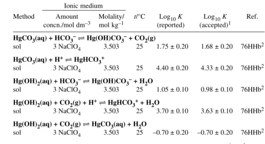
Table 3 Recommended values¹for the Hg²⁺– CO₃^2–system at 298.15 K, 1 bar, and I_m= 0 mol kg^–1. R = Recommended; P = Provisional.

Reaction

Hg(OH)₂(aq) + CO₂(g) HgCO₃(aq) + H₂O log₁₀K° = –0.70 ± 0.20 R Hg(OH)₂(aq) + HCO₃^–Hg(OH)CO₃^–+ H₂O log₁₀K° = 0.98 ± 0.10 R Hg(OH)₂(aq) + CO₂(g) + H⁺HgHCO₃⁺+ H₂O log₁₀K° = 3.63 ± 0.10 R HgCO₃.2HgO(s)+3H₂O 3Hg(OH)₂(aq) +CO₂(g) log₁₀K_s = –11.27 ± 0.35 P

1The value for log₁₀K_srefers to I_c= 3.0 mol dm^–3(NaClO₄).

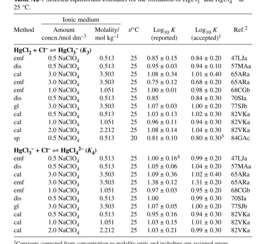
Table 4 Selected values for the Hg²⁺– PO₄^3–system at 298.15 K, 1 bar, and I_c= 3 mol dm^–3 NaClO₄.

Reaction

Hg²⁺+ HPO₄^2–HgHPO₄(aq) log₁₀K = 8.8 ± 0.2 Hg²⁺+ HPO₄^2–HgPO₄^–+ H⁺ log₁₀K = 3.25 ± 0.2 Hg₃(PO₄)₂(s) + 2H⁺3Hg²⁺+ 2HPO₄^2– log₁₀*K_s= –24.6 ± 0.6 (HgOH)₃PO₄(s) + 4H⁺3Hg²⁺+ HPO₄^2–+ 3H₂O log₁₀*K_s= –9.4 ± 0.8 HgHPO₄(s) Hg²⁺+ HPO₄^2– log₁₀K_s = –13.1 ± 0.1

Table 5 Selected stability constants for the Hg²⁺– SO₄^2–

system at 298.15 K, 1 bar, and I_c= 0.50 mol dm^–3NaClO₄. Reaction

Hg²⁺+ SO₄^2–HgSO₄(aq) log₁₀K₁= 1.4 ± 0.1 P Hg²⁺+ 2SO₄^2–Hg(SO₄)₂^2– log₁₀β₂= 2.4 ^a

a= of doubtful value, unknown uncertainty.

Tables 6 and 7 report Recommended values for the protonation constants for CO₃^2–and PO₄^3–. These are supplementary data that are required to complete speciation calculations on the related Hg²⁺

systems. These data, and the reaction ion interaction coefficients, ∆ε, are also derived from the critical evaluation of published stability constants [2003PET] and application of SIT functions. However, the reader is alerted to the fact that NaCl medium and different activity coefficient relationships are used for these two systems (see Sections 7.1 and 7.2).

Table 2 (Continued).

Reaction

Table 6 Recommended values for the H⁺– CO₃^2–system at 298.15 K, 1 bar, and I_m= 0 mol kg^–1. R = Recommended; P = Provisional. ∆εvalues for NaCl medium.

Reaction

H⁺+ CO₃^2–HCO₃^– log₁₀K₁° = 10.336 ± 0.005 R

∆ε¹ = –(0.116 ± 0.002) kg mol^–1 H⁺+ HCO₃^–H₂CO₃*³ log₁₀K₂° = 6.355 ± 0.003 R

∆ε² = –(0.092 ± 0.002) kg mol^–1

1Based on regression analysis yielding a_jB = 1.117 ± 0.015. With a_jB = 1.50, log₁₀ K₁° = 10.248 ± 0.002, and ∆ε = –(0.078 ± 0.001) kg mol^–1. See Section 7.1.

2Based on regression analysis yielding a_jB = 1.136 ± 0.022. With a_jB = 1.50, log₁₀ K₂° = 6.317 ± 0.001, and ∆ε = –(0.072 ± 0.001) kg mol^–1.

3[H₂CO₃*] = [CO₂(aq)] + [H₂CO₃].

Table 7 Recommended values for the H⁺– PO₄^3–system at 298.15 K, 1 bar, and I_m= 0 mol kg^–1. R = Recommended; P = Provisional. ∆εvalues for NaCl medium.

Reaction

H⁺+ PO₄^3–HPO₄^2– log₁₀K₁° = 12.338 ± 0.028 R

∆ε¹ = –(0.078 ± 0.019) kg mol^–1 H⁺+ HPO₄^2–H₂PO₄^– log₁₀K₂° = 7.200 ± 0.008 R

∆ε² = –(0.061 ± 0.016) kg mol^–1 H⁺+ H₂PO₄^–H₃PO₄ log₁₀K₃° = 2.141 ± 0.010 R

∆ε³ = –(0.043 ± 0.017) kg mol^–1

1Based on regression analysis yielding a_jB = 1.204 ± 0.090. With a_jB = 1.50, log₁₀ K₁° = 12.277 ± 0.019, and ∆ε = –(0.029 ± 0.008) kg mol^–1. See Section 7.2.

2Based on regression analysis yielding a_jB = 1.160 ± 0.083. With a_jB = 1.50, log₁₀ K₂° = 7.191 ± 0.008, and ∆ε = –(0.011 ± 0.007) kg mol^–1.

3Based on regression analysis yielding a_jB = 1.352 ± 0.235. With a_jB = 1.50, log₁₀ K₂° = 2.138 ± 0.009, and ∆ε = –(0.033 ± 0.006) kg mol^–1.

The abbreviations used to describe the experimental methods are as follows.

emf emf measurements using electrodes utilizing redox equilibria sol solubility determination

gl pH measurement by glass electrode con conductivity

dis distribution between immiscible solvents

ise emf measurements using an ion selective electrode cal calorimetry

sp spectrophotometry

4. Hg(II) SOLUTION CHEMISTRY

Mercury has two common cations in aqueous solution, a di-ion, Hg₂²⁺, composed of two singly charged ions, and a doubly charged Hg²⁺. Of these, Hg(II) is the dominant form in most aqueous solutions.

Diagrams of pH-potential boundaries indicate that Hg(I) is stable only within a narrow band of E_Hval- ues in acid solutions [66ZOU]. The hydrolysis reactions of Hg(II) are significant at pH > 1 [86BAE], and these reactions must be taken into account in all equilibrium studies of Hg²⁺-ligand systems. At low

aqueous mercury concentrations (≤0.01 mmol dm^–3), the dominant hydrolysis species formed are monomers HgOH⁺and Hg(OH)₂(aq), while Hg(OH)₃^–forms at pH > 13. At higher mercury concen- trations, evidence for the formation of the dimer, Hg₂(OH)₂²⁺, has been reported [62AHa, 77SJb].

5. DATA EVALUATION METHODS 5.1 Data evaluation criteria

The majority of anion complexation studies of Hg(II) have utilized the potentiometric technique and have been carried out using sodium perchlorate as the ionic medium. A few have used [Ca,Mg](ClO₄)₂ or [Na,K]NO₃, but the propensity of Hg²⁺to form stable chloro complexes precludes use of chloride media.

In this review, stability constant and reaction enthalpy data published for 25 °C and a wide range of ionic strengths (I_cor I_m) have been used in weighted linear regression analyses to determine values valid at 298.15 K and I_m= 0 mol kg^–1. Literature data have been accepted as “reliable” (designated “re- ported” in relevant tables), and thus included in the regression analysis, when all, or in some cases most, of the following requirements have been met:

i. full experimental details are reported (solution stoichiometry, electrode calibration method, tem- perature, ionic strength, error analysis);

ii. the equilibrium model is considered to be complete (including hydrolysis reactions);

iii. data are for an essentially noncomplexing medium; and

iv. the experimental method and numerical analysis are considered to have minimal systematic er- rors.

These are not the usual IUPAC criteria for selection of published data that are used in the calcu- lation of “Recommended” and “Provisional” values at a single ionic strength [2001PRa], but they per- mit utilization of a larger data set for the adopted ionic strength correlations.

Most of the uncertainties reported in the literature reflect analytical and numerical precision, but do not include systematic errors. We assign an additional uncertainty to each selected value that reflects our estimation of accuracy and reliability of the experimental methods. The data selected for use in the SIT analyses for Hg²⁺complexes are recorded in Tables A2-1 through A2-15 in Appendix 2. The ta- bles record only those data that have met our selection criteria. The column headed log₁₀K (reported) contains the “accepted” stability constant data, on the molar scale, as published. The column headed log₁₀K (accepted) contains the same data converted to the molal scale (to facilitate SIT analysis). It in- dicates our assigned uncertainties, which are based on the reliability and systematic uncertainties of the data. In the SIT regression analysis, the constants are weighted according to these assigned uncertain- ties. References that contain data rejected from our analysis are recorded in the footnotes to relevant ta- bles. Each reference carries superscript(s) that refer to the reasons for rejection of the data according to the alphabetic list below.

Reasons for rejection of specific references include:

a. data are for temperature(s) other than 25 °C, data cannot be corrected to 25 °C, or the tempera- ture is not defined;

b. data for Hg²⁺complexation are for a medium other than (Na)ClO₄; c. the ionic strength has not been held constant;

d. experimental details are incomplete;

e. the equilibrium model is incomplete;

f. electrode calibration details are missing;

g. incomplete experimental data;

h. the description of the numerical analysis of measurement data is incomplete;

i. the correction for competing equilibria [e.g., formation of Hg(OH)₂(aq)] is inadequate; and j. value(s) appear to be in error when compared with results from more than one other reliable lab-

oratory.

Of this list, a and b do not necessarily question the quality of the data, but merely indicate that the data has not been used in the present review. The remaining reasons, however, place doubt in rela- tion to the validity of the data in question.

5.2 Methods for numerical extrapolation of data to I_m= 0 mol kg^–1

For many reactions, equilibrium measurements cannot be made accurately, or at all, in dilute solutions (which would permit calculation of standard state values by application of simple activity coefficient relationships). Such is the case for reactions involving formation of weak complexes or ions of high charge. For these systems, precise equilibrium data can only be obtained in the presence of an inert elec- trolyte of sufficiently high concentration to ensure that reactant activity coefficients are reasonably con- stant. The associated short-range, weak, noncoulombic interactions between the reactant species and electrolyte anions or cations must be considered. They may be described in terms of ion pair formation (as required when the Debye–Hückel theory or the empirical Davies equation is used for activity co- efficients). Alternatively, they can be quantified by inclusion of empirical specific ion interaction coef- ficients, ε(i,k), within the activity coefficient expression, as in the Brønsted–Guggenheim–Scatchard (SIT) model [97PUI], which is adopted in this review:

log₁₀γ_m,i= – z_i²A√I_m(1 + a_jB√I_m)^–1+ Σ_kε(i,k) m_k

= – z_i²D + Σ_kε(i,k) m_k (1)

In this model, the ionic strength is expressed on the molality scale, I_m. The advantage of SIT is that the activity coefficient expressions are valid over a very wide range of concentrations. In contrast, the Debye–Hückel and Davies equations are limited to I_m0.03 mol kg^–1and < 0.1 mol kg^–1, respectively.

The ionic strength dependence of stability constants discussed in this report does not require empirical relationships more complex than eq. 1. Use of Pitzer equations would require adoption of data that have not undergone critical review. The present critical assessment of data could, however, be used to refine the Pitzer model for its application to complex, multicomponent systems.

The following general reaction is assumed (omitting most charges for simplicity):

pM + qL + rH₂O M_pL_q(OH)_r+ rH⁺

If the stability constant β_p,q,ris determined in an ionic medium (containing the 1:1 electrolyte NX of ionic strength I_mmol kg^–1) and expressed in units of relative molality [m(species i)/m°, where the stan- dard molality m° = 1 mol kg^–1] it is related to the corresponding value at zero ionic strength, β_p,q,r°:

log₁₀β_p,q,r= log₁₀β_p,q,r° + plog₁₀γ_m(M) + qlog₁₀γ_m(L) + rlog₁₀a(H₂O)

– log₁₀γ_m(p,q,r) – rlog₁₀γ_m(H⁺) (2)

where γ_m(p,q,r) refers to the species M_pL_q(OH)_r.

Substitution of eq. 1 into 2, and the assumption that the concentration of NX is much greater than that of each reactant (such that I_m= m_k), gives

log₁₀β_p,q,r– ∆z²D – rlog₁₀a(H₂O) = log₁₀β_p,q,r° – ∆εI_m (3) where

∆z²= (pz_M+ qz_L– r)²+ r – p(z_M)²– q(z_L)² and

∆ε= ε(complex, N⁺or X^–) + rε(H⁺, X^–) – pε(M⁺, X^–) – qε(L^–, N⁺)

In this review, the term a_jB is set at 1.5 kg^1/2mol^–1/2, except for the systems H⁺– CO₃^2–and H⁺– PO₄^3–, in which it is treated as a variable in the regression analysis using eq. 3. The term log₁₀a(H₂O) is near constant for most studies of equilibrium in dilute aqueous solutions where the ionic medium is in large excess; also, log₁₀a(H₂O)→0 as I_m→0 mol kg^–1. For a 1:1 electrolyte (NX), this term can be calculated from the solution osmotic coefficient, Φ_m, if the minor electrolyte species (the reacting ions) are neglected, whence I_m≈m(NX):

log₁₀a(H₂O) = –2m(NX)Φ_m/M_W(ln 10)

Values for the osmotic coefficient of NaClO₄media are available in [59ROB]; these provide the relationship log₁₀a(H₂O) = –(0.01378 ± 0.00003)(I_m/mol kg^–1) for NaClO₄media at 25 °C (298.15 K), I_m= 0 to 3.5 mol kg^–1.

The application of SIT to the selected literature stability constants involves graphical extrapola- tion of log₁₀β_p,q,r– ∆z²D – rlog₁₀a(H₂O) to m_k= 0 (or I_m= 0 mol kg^–1for a system with a large ex- cess of 1:1 electrolyte), using eq. 3. The intercept at I_m= 0 mol kg^–1gives the standard equilibrium con- stant log₁₀ β_p,q,r°, and the slope provides the reaction ion interaction coefficient (slope = –∆ε) as defined in eq. 3. If the regression line slope is negative, then ∆εis positive. Conversely, the value of the stability constantβ_p,q,rat a specific ionic strength, I_m, can be calculated from β_p,q,r° if the value of the empirical parameter ∆εis known. Thus, this review reports values for both log₁₀β_p,q,r° and ∆ε. [It is noted that in eq. 3, D is a function of I_m, whereas the ion interaction term (i.e., Σ_kε(i,k) m_k; eq. 1) is a function of m_k; however, m_k≈I_mfor a medium containing excess 1:1 electrolyte.]

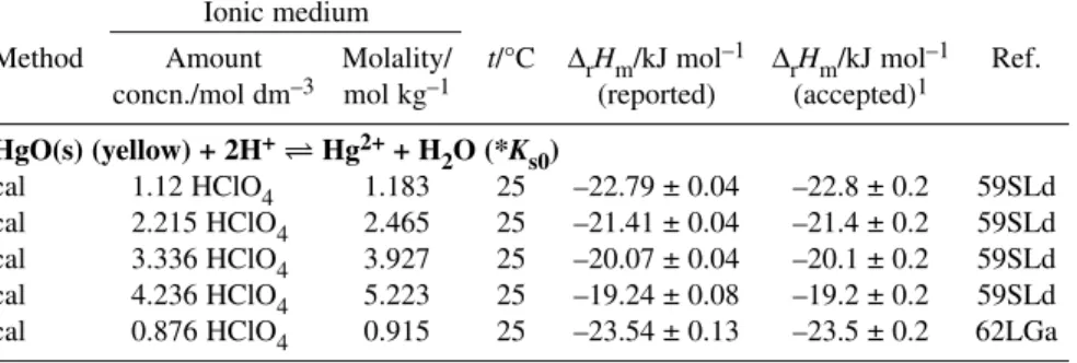
The weighted linear regression analyses using SIT are represented graphically and are recorded in Appendix 3 (e.g., Fig. A3-1). The SIT regressions used values that resulted from independent analy- ses of experimental datum points (population values). Some values have very strong experimental bases, other have weaker grounds, some are based on a few, others on a large number of datum points, and the experimental methods also may differ. These differences were taken into account in the regres- sion analyses by assigning appropriate weights to each value, according to [92GRE, Appendix C]. A specific regression analysis could only include values that belong to the same “parent distribution”, which means they must be “consistent” with each other. In this document, “consistency” was estab- lished by propagating the uncertainties of the regression results (at I_m= 0 mol kg^–1) back to high ionic strengths, viz. the dotted lines in Fig. A3-1. If the initial SIT analysis revealed values for which the un- certainty ranges did not overlap with the area between the dotted lines, they were considered to be in- consistent with the population; thus, they were removed (as outliers) or, if justified, their uncertainties were increased accordingly. For the figures in Appendix 3, the error propagation calculation that deter- mined the confidence limits that are shown used the errors on log₁₀β_p,q,r°, and on ∆εobtained in the final SIT regression.

5.3 Criteria for the assignments: “Recommended” and “Provisional”

Criteria for assigning equilibrium data as “Recommended” or “Provisional” (previously “Tentative”) were based on those used in more recent IUPAC critical reviews [97SJa, 97LPa, 2001PRa]. In most ex- amples in this work, an equilibrium constant log₁₀β_p,q,r° was classified as “Recommended” if the stan- dard deviation, σ, (obtained from the SIT regression) was ≤0.2, and as “Provisional” if 0.2 ≤σ ≤0.4.

Values for ∆_rH_m° obtained from the SIT regression were assigned as “Recommended” if σ ≤ 2.0 kJ mol^–1, and as “Provisional” if 2.0 ≤σ ≤5.0 kJ mol^–1. In some cases, the assignment “Provisional” was necessary because there were too few “accepted” data to allow a reliable regression analysis. However, in others more subjective judgement was used when, for example, further experimental confirmation was needed or the result is, despite good coincidence of experimental data, an unexpected one.

6. EVALUATION OF EQUILIBRIUM CONSTANTS (HOMOGENEOUS REACTIONS) 6.1 The Hg²⁺– OH^–system

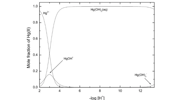
The speciation diagram for the Hg²⁺– OH^–system, based on the Recommended values recorded in Table 1 for stability constants at I_m= 0 mol kg^–1, is shown in Fig. 1. Results outside the pH range 2 to 12 should be viewed with caution as activity coefficients may deviate significantly from 1.0.

6.1.1 Formation of HgOH⁺

Formation of the first mononuclear hydrolysis species is described by eq. 4,

Hg²⁺+ H₂OHgOH⁺+ H⁺ (4)

Data selected for the SIT analysis, to determine the stability constant at zero ionic strength (the stan- dard equilibrium constant) and the reaction interaction coefficient ∆ε(4), are listed in Table A2-1, along with references and our assigned uncertainties. The selected data refer to perchlorate media and 25 °C.

References for rejected data are shown in the footnote, along with the reasons for rejection, designated by the superscript letters specified in Section 5.1. The uncertainties assigned to the selected data are used to determine the weight for each respective value. The weighted linear regression (Fig. A3-1) in- volves the expression

log₁₀*K₁+ 2D – log₁₀a(H₂O) = log₁₀*K₁° – ∆εI_m

that is derived from eqs. 3 and 4 (∆z²= –2) and which yields log₁₀*K₁° from the intercept and –∆ε from the slope. It indicates reasonable consistency among the data and provides the Recommended value

log₁₀*K₁° (eq. 4, 298.15 K) = –3.40 ± 0.08

Fig. 1 Speciation diagram for the binary Hg(II) hydroxide system as obtained from the Recommended stability constants at I_m= 0 mol kg^–1(Table 1). This diagram is applicable for Hg(II) concentrations ≤0.01 mmol dm^–3. Results outside the –log [H⁺] range of 2 to 12 should be viewed with caution as activity coefficients deviate from 1.0.

This value is identical to that selected by Baes and Mesmer [86BAE] in their review of the hydrolysis of metal ions; their value was based on a smaller and older set of stability constants. The value for ∆ε(4) is –(0.14 ± 0.03) kg mol^–1. The values for ε(Hg²⁺,ClO₄^–) = (0.34 ± 0.03) kg mol^–1and ε(H⁺,ClO₄^–) = (0.14 ± 0.02) kg mol^–1[97GRE] lead to ε(HgOH⁺,ClO₄^–) = (0.06 ± 0.05) kg mol^–1.

6.1.2 Formation of Hg(OH)₂(aq)

Formation of the second mononuclear hydrolysis species is described by eq. 5,

Hg²⁺+ 2H₂OHg(OH)₂(aq) + 2H⁺ (5)

Data selected for the SIT analysis, and our estimated uncertainties, are listed in Table A2-2. References for rejected data are shown in the footnote. The selected stability constants were determined at 25 °C in sodium or calcium perchlorate media of constant ionic strength. Figure A3-2 illustrates that there is a relatively large scatter of data at high ionic strength. It appears that the data obtained from calcium perchlorate media [62AHa] and from solubility experiments [61DTa] may be less reliable than the other data obtained at I_c= 3.0 mol dm^–3. The experimental methodology used by [62AHa] resulted in some changes in the ionic strength, whereas the work of [61DTa] potentially suffers from lack of character- ization of the solid phase. The Recommended constant at zero ionic strength, derived from the weighted linear regression, is

log₁₀*β₂° (eq. 5, 298.15 K) = –5.98 ± 0.06

The reaction ion interaction coefficient ∆ε(5) = –(0.14 ± 0.02) kg mol^–1. The values for ε(Hg²⁺,ClO₄^–)

= (0.34 ± 0.03) kg mol^–1 and ε(H⁺,ClO₄^–) = (0.14 ± 0.02) kg mol^–1 [97GRE] lead to ε(Hg(OH)₂,Na⁺,ClO₄^–) = –(0.08 ± 0.05) kg mol^–1. This value is consistent with that reported by [90CIA], –(0.06 ± 0.05) kg mol^–1. The standard equilibrium constant recommended in this review is somewhat more positive than that evaluated by Baes and Mesmer [86BAE] (log₁₀*β₂° = –6.17), but in good agreement with the value proposed by Ciavatta [90CIA] (log₁₀*β₂° = –6.01).

6.1.3 Formation of Hg(OH)₃^–, Hg₂OH³⁺, and Hg₂(OH)₂²⁺

Reliable stability constant data have been reported for the formation of Hg(OH)₃^–, Hg₂OH³⁺, and Hg₂(OH)₂²⁺(Table A2-3). However, there are insufficient data for a SIT analysis. From the stability constant for Hg(OH)₃^–determined at I_m= 0 mol kg^–1[38GHa] and the stability constant for Hg(OH)₂ (log₁₀*β₂° = –5.98), the stepwise stability constant log₁₀*K₃° = –15.13 is calculated. This species will form only in highly alkaline solutions; it is unlikely to be environmentally important. The species Hg₂OH³⁺and Hg₂(OH)₂²⁺will form only at relatively high Hg(II) concentrations (ca. 0.005 mol dm^–3);

they also are unlikely to be environmentally important.

There has been some conjecture in relation to the stoichiometry of the Hg_n(OH)_nⁿ⁺ species.

Sjöberg [77SJb] found evidence for Hg₂(OH)₂²⁺, consistent with the above. In contrast, Baes and Mesmer [86BAE], in recalculating the data of Ahlberg [62AHa], concluded that the polymeric species is Hg₃(OH)₃³⁺. Regardless of the stoichiometry, evidence for this polymer has only been found in 3 mol dm^–3perchlorate media and, as such, it is not possible to determine a stability constant at zero ionic strength. The polymeric species Hg₄(OH)₃⁵⁺, also postulated [62AHa], has not been identified in any other study; as such, its existence is not accepted by this review.

6.2 The Hg²⁺– Cl^–system

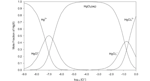
The speciation diagram for the Hg²⁺– Cl^–system, based on the Recommended values for stability con- stants at I_m= 0 mol kg^–1(Table 2), is shown in Fig. 2, which represents the situation in which hydrol- ysis is suppressed (pH < 2). Results for values of log₁₀[Cl^–] > –2.0 should be viewed with caution as activity coefficients may deviate significantly from 1.0. Formation of the chloro complexes in aqueous solution is described by eqs. 6–9

Hg²⁺+ Cl^–HgCl⁺ (6)

Hg²⁺+ 2Cl^–HgCl₂(aq) (7)

HgCl₂(aq) + Cl^–HgCl₃^– (8)

HgCl₃^–+ Cl^–HgCl₄^2– (9)

The 1:1 and 1:2 chloro complexes of Hg(II) are among the most stable of metal-chloro complexes formed.

Many of the early stability constant data are not reliable because the constant ionic strength pro- tocol was not employed. Furthermore, the simultaneous presence of HgCl₂, HgCl₃^–, and HgCl₄^2–was not recognized, which led to erroneous evaluations. A comprehensive investigation of the Hg(I) and Hg(II) chloride system was undertaken by Sillén in the 1940s. Since [Hg²⁺] cannot be measured directly with a Hg electrode, due to formation of Hg(I), Sillén developed an indirect but very precise emf method based on measurement of the redox potential for Hg(II)/Hg(I) in the presence of Hg₂Cl₂(s).

These experiments, performed at 25.0 °C, I_c= 0.5 mol dm^–3(NaClO₄) and pH = 2 (to avoid hydroly- sis), are described in detail in [46SIL].

6.2.1 Formation of HgCl⁺

Data selected for the SIT analysis, to determine the stability constant at zero ionic strength (the stan- dard equilibrium constant) and the ion interaction coefficient ∆εfor reaction 6, are listed in Table A2-4, along with our assigned uncertainties. The selected data all refer to NaClO₄media and 25 °C. The weighted linear regression (Fig. A3-3) shows that there is reasonable consistency between the data and results in the Recommended standard constant

log₁₀K₁° (eq. 6, 298.15 K) = 7.30 ± 0.05

Fig. 2 Speciation diagram of the binary Hg(II) chloride system as obtained from the Recommended stability constants at I_m= 0 mol kg^–1, Table 2. Hydrolysis is suppressed (pH < 2 is assumed). Results for –log [Cl^–] > –2.0 should be viewed with caution as activity coefficients deviate from 1.0.

The reaction ion interaction coefficient based on this regression is ∆ε(6) = –(0.22 ± 0.04) kg mol^–1, which is in excellent agreement with that calculated from tabulated ε values [97GRE] for the re- actant and product species, ∆ε(6) = –(0.18 ± 0.06) kg mol^–1.

Formation of HgCl⁺is also expressed by reaction 10

Hg²⁺+ HgCl₂(aq)2HgCl⁺ (10)

The emf method elaborated by Sillén [46SIL, 47SIL] yields a redox titration curve that goes through a maximum of dE/dc (where c is the concentration of titrant) when the concentration of HgCl⁺ is at a maximum, because the measured emf is a function of [HgCl⁺] alone. This results in precise log K values for equilibrium 10. The selected values for 25 °C and (Na,H)ClO₄media are listed in Table A2-5. With the exception of one solvent extraction (distribution) study [57MAa], all values result from application of Sillén’s emf method. The weighted linear regression (Fig. A3-4) results in the recom- mended value of:

log₁₀K° (eq. 10, 298.15 K) = 0.61 ± 0.03

The reaction ion interaction coefficient is ∆ε(10) = –(0.02 ± 0.02) kg mol^–1. 6.2.2 Formation of HgCl₂(aq)

Data selected for the SIT analysis of reaction 7 are listed in Table A2-6. The weighted linear regression (Fig. A3-5) shows that there is reasonable consistency between the data and results in the Recommended standard constant

log₁₀β₂° (eq. 7, 298.15 K) = 14.00 ± 0.07

The resulting reaction ion interaction coefficient is ∆ε(7) = –(0.39 ± 0.03) kg mol^–1.

From the reported values ε(Hg²⁺,ClO₄^–) = (0.34 ± 0.03) kg mol^–1, ε(HgCl⁺,ClO₄^–) = (0.19 ± 0.02) kg mol^–1, and ε(Cl^–,Na⁺) = (0.03 ± 0.01) kg mol^–1[97GRE], ∆ε(10) gives ε(HgCl₂,Na⁺,ClO₄^–)

= (0.06 ± 0.05) kg mol^–1and ∆ε(7) gives ε(HgCl₂,Na⁺,ClO₄^–) = (0.01 ± 0.04) kg mol^–1. Both values are consistent with that reported by [90CIA], (0.06 ± 0.03) kg mol^–1.

The evaluated constants for reactions 6, 7, and 10 define an energy cycle that is consistent within experimental error. From the relationship 2log₁₀K₁°(6) = log₁₀K°(10) + log₁₀β₂°(7), we derive the Recommended standard constant

log₁₀K₁° (eq. 6, 298.15 K) = 7.31 ± 0.04

which is consistent with that derived from the SIT analysis (Section 6.2.1).

6.2.3 Formation of HgCl₃^–and HgCl₄^2–

The stepwise formation constants for the 1:3 and 1:4 Hg(II) chloro complexes are much smaller than those for the 1:1 and 1:2 complexes. Thus, comparatively large chloride concentrations are required for them to form (Fig. 2). Nevertheless, their stabilities are such that they always exist in aqueous so- lution simultaneously, in equilibrium with HgCl₂(aq). Data selected for the SIT analyses for reactions 8 and 9 are listed in Table A2-7. The weighted linear regression analyses (Figs. A3-6 and A3-7) indi- cate excellent consistency between the data. They result in the Recommended standard constants (I_m= 0 mol kg^–1):

log₁₀K₃° (eq. 8, 298.15 K) = 0.92₅± 0.09 log₁₀K₄° (eq. 9, 298.15 K) = 0.61 ± 0.12

The resulting reaction ion interaction coefficients are ∆ε(8) = (0.01 ± 0.05) kg mol^–1and ∆ε(9) = –(0.00₃± 0.05) kg mol^–1. From these, we derive new εvalues: ε(Na⁺, HgCl₃^–) = (0.05 ± 0.07) kg mol^–1 and ε(Na⁺, HgCl₄^2–) = (0.08 ± 0.09) kg mol^–1.