39 Johannes Siegfried Samir Najjar

(1)

D is se rt at io ns re ih e P hy si k - B an d 3 9 Johannes Kar ch

Nucleon structure from stochastic estimators Johannes Siegfried

Samir Najjar

39

9 783868 451092

ISBN 978-3-86845-109-2 ISBN 978-3-86845-109-2

from first principle through the computation of baryon three-point functions with lattice QCD. The numerical effort involved in such computations is sizable and thus an efficient algorithm that extracts most information at given cost is highly desirable.

In this work we demonstrate that stochastic estimation techniques can substantially increase the information/cost ratio. We examine the available results at N_f = 2 for the nucleon axial coupling g_A and iso-vector quark momentum fraction <x>_u-d from various collabora- tions and compare them to the experimental values. The tension between them is attributed to excited state contributions (ESCs).

We furthermore study the impact of ESCs in moments of GPDs through a model fit. This model also deals with the effects of the choice of parameters used in the computation, like the source-sink separation t_sink.

We demonstrate that the choice of t_sink by the Regensburg group in previous studies was reasonable and cannot account for discrepan- cies with the experiment.To reduce the excited state contributions in two-point functions, and consequently three-point functions, we suggest a non-Gaussian quark smearing. This is a linear combination of two Gaussian smearings with one free parameter, which can be tuned to an optimal choice with a fit.

(2)

Johannes Siegfried Samir Najjar

Nucleon structure from stochastic estimators

(3)

Herausgegeben vom Präsidium des Alumnivereins der Physikalischen Fakultät:

Klaus Richter, Andreas Schäfer, Werner Wegscheider

Dissertationsreihe der Fakultät für Physik der Universität Regensburg, Band 39

Dissertation zur Erlangung des Doktorgrades der Naturwissenschaften (Dr. rer. nat.) der naturwissenschaftlichen Fakultät II - Physik der Universität Regensburg vorgelegt von

Johannes Siegfried Samir Najjar aus Kelheim

im Jahr 2014

Die Arbeit wurde von Prof. Dr. G. Bali angeleitet.

Das Promotionsgesuch wurde am 18.11.2013 eingereicht.

Das Kolloquium fand am 06.05.2014 statt.

Prüfungsausschuss: Vorsitzender: Prof. Dr. C. Back 1. Gutachter: Prof. Dr. G. Bali 2. Gutachter: Prof. Dr. V. Braun weiterer Prüfer: Prof. Dr. J. Fabian

(4)

Johannes Siegfried Samir Najjar

Nucleon structure from

stochastic estimators

(5)

in der Deutschen Nationalbibliografie. Detailierte bibliografische Daten sind im Internet über http://dnb.ddb.de abrufbar.

1. Auflage 2014

Umschlagentwurf: Franz Stadler, Designcooperative Nittenau eG Layout: Johannes Siegfried Samir Najjar

Druck: Docupoint, Magdeburg ISBN: 978-3-86845-109-2

Weitere Informationen zum Verlagsprogramm erhalten Sie unter:

(6)

Introduction 1

1.1. Motivation

The Standard model of particle physics consists of the joint description of the electro- weak [11] forces and the strong interaction [22, 33, 44]. Although it has some shortcomings, like the absence of gravity in the theory, it is very successful in describing the spectrum of observed particles and their interactions. The recent discovery of the Higgs boson [55]

was long awaited and the search for it was the main goal of building theLarge Hadron Collider(LHC). Mathematically speaking the Standard model is a quantum field theory of the groupsSU(2)⊗U(1)⊗SU(3), where the strong interaction is described by the color groupSU(3). Thus it is calledquantum chromodynamics(QCD). Its gauge bosons are thegluonsand their self interaction makes the theory non-linear. This complicates analytical computations at low energies, but as QCD displaysasymptotic freedom[33] at higher energy scales perturbative expansions are possible.

For low energy properties of quark bound states,hadrons[66], non-perturbative methods are imperative. The approach chosen in this work is calledlattice QCD(LQCD). Here we introduce a discrete spacetime lattice and perform Monte Carlo simulations to evaluate the path integral. The finite lattice spacing serves as an ultraviolet cut-off and the finite volume as an infrared regularization. Thus there are no divergences in the theory. The limit of infinite lattice size and vanishing lattice spacing is well defined and regularized continuum QCD is recovered [77].

LQCD has produced many convincing results¹¹. A widely recognized achievement was the computation of the proton mass and the light hadron spectrum from first principles [88].

1There are many more results, also in different research areas like finite temperature LQCD, but we focus on hadron structure here.

(11)

1.2. Objectives

The objectives of this work lie in the improvement of the algorithms and parameter choices in the computation of nucleon masses and three-point functions²², which are needed, e.g., to compute (generalized) form factors.

The primary goal was to find a method which performs well at high momentum trans- fers and utilizes as many different lattice momenta as possible. A natural candidate for this is the stochastic estimation of the –otherwise sequentially computed– propagator between the current insertion and the baryon sink.

Within the computation of three-point functions the baryon source sink distance in Eu- clidean time (tsink) is fixed and this choice entails certain systematic effects. An estimation of these effects is necessary to enable judgment on how reliable the obtained data are.

The excited state contributions plague the extraction of ground state properties, and it is crucial to suppress these excitations as much as possible without compromising the signal-to-noise ratio. Therefore a new ansatz for quark smearing which fulfills these prerequisites is desirable.

1.3. Outline

This work focuses on technical aspects of the computation of nucleon properties. It contains several distinct topics and is structured in the following way. In Chapter 22 we will present an introduction to nucleon structure and the observables we use to parameterize it. The methods and techniques needed to compute these observables are presented in Chapter 33.

The lattice community has struggled to reach agreement on nucleon structure parameters with the experiment. With the progress in algorithms and computer power ever lighter pion masses and even some simulations at the physical point are possible. Still a tension between some lattice results and experimental observations persists, and one explanation for that is the presence of excited state contributions in the lattice data.

This is illustrated for the examples of the nucleon axial coupling and the iso-vector quark momentum fraction in the nucleon in Chapter 44.

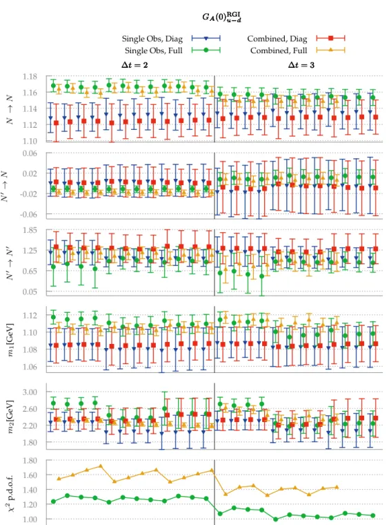
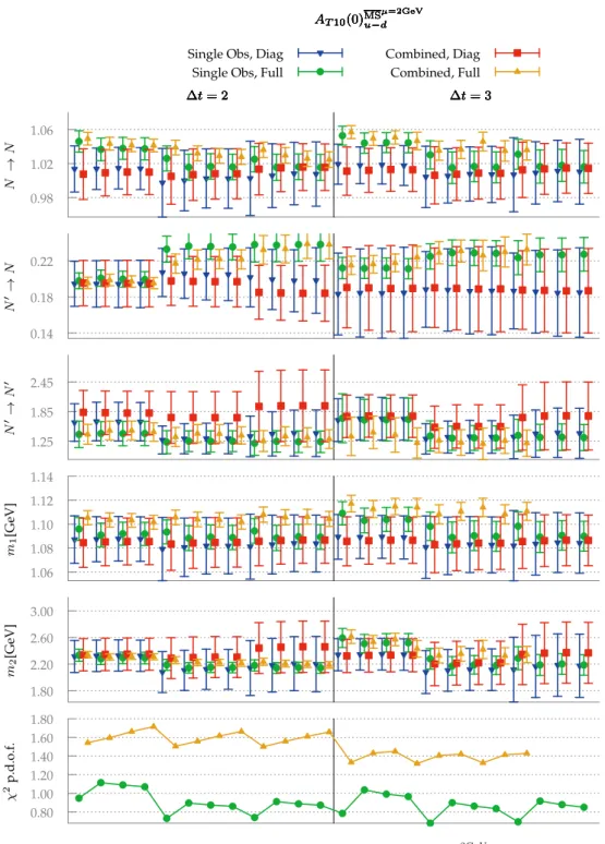
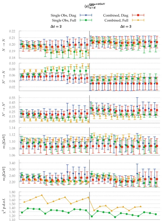
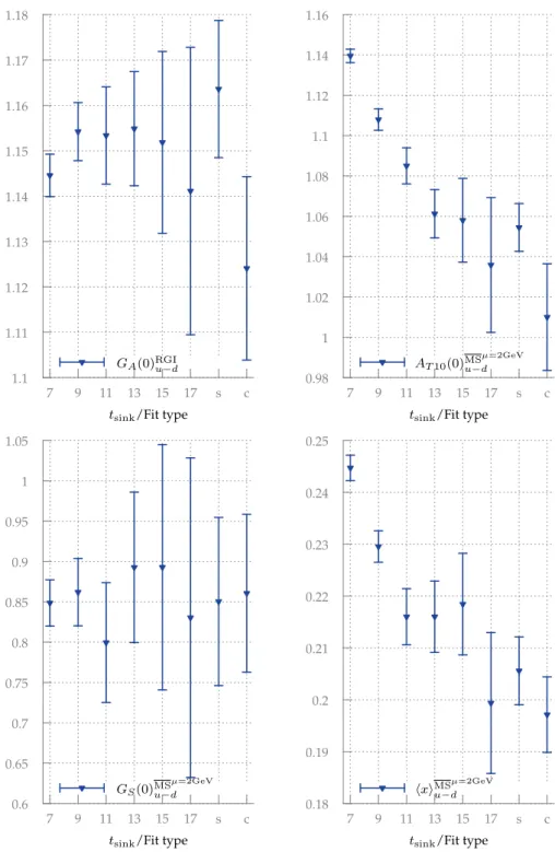
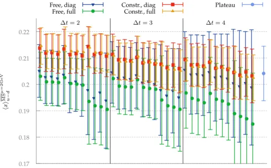
In Chapter 55 an excited state analysis is performed of data from one ensemble with multiple values fort_sink, and it is found that the choice made fort_sink on other ensem- bles is sufficient to suppress the excited state contributions when the quark smearing is sufficiently optimized.

2In lattice QCD one computes correlators between a hadron source at a spacetime point and a hadron sink. The energy of the hadron can then be extracted from this correlation function, and this is referred to as two-point function. The presence of a current insertion defines a third point and hence the name three-point function.

(12)

1.3. Outline The computation of three-point functions on the lattice is conventionally done with the use ofsequential sources. To compute such a sequential source one has to fix the sink momentum of the hadron. In Chapter 66a new algorithm to compute these three-point functions with the help of stochastic estimator techniques is explained, and the benefits of having multiple sink momenta are shown in an exemplary computation of nucleon (generalized) form factors.

The quark level smearing discussed earlier is an essential ingredient in suppressing excited state contributions sufficiently to extract reliable ground state properties. The quality of the employed smearing and possible ways to improve it with a non-Gaussian gauge covariant smearing method is outlined in Chapter 77.

A summary is provided in Chapter 88.

(13)

(14)

Hadron structure in continuum QCD 2

The road that lead to the development of QCD was rather complex, but it has always been driven by the results of collider experiments and the so found non-trivial inter- nal structure of hadrons. Some of the properties of the nucleon, like its charge radius, see Section 2.4.22.4.2, are not fully understood experimentally. For the charge radius a computation of it from first principles is highly desirable.

Another experiment with at the time surprising result was the measurement of the contribution of the quarks to the proton spin. In [99] the European Muon Collaboration (EMC) found that the quarks do not carry all the proton spin, contrary to naive ex- pectations. This lead to the proton spin puzzle or spin crisis, see Section 2.4.32.4.3for the individual hadron contrubutions to the proton spin.

In this section we classify the structure of the nucleon in a set of functions and show how they correspond to quantities which are accessible via lattice QCD computations.

2.1. Nucleon Structure

The parton model describes the nucleon at very high energy as a conglomeration of non-interacting quanta, i .e., its partons. A very extensive review about the structure of hadrons is given in [1010] and we follow the derivations therein. These partons require a quantum mechanical treatment and thus they cannot be simply described by a proba- bility to find one in a given state. Nevertheless it is possible to define analogs of Wigner distributions for them, and these are called generalized parton distributions (GPDs)¹¹. Experimentally GPDs are accessible in, e.g., deeply virtual Compton scattering (DVCS) or deeply virtual meson production.

Compton scattering is an elastic scattering of an electron off a nucleon producing a photon. They exchange a virtual photon and if the energy of that photon is high enough (deeply virtual) it is sensitive to the inner structure of the nucleon, see Fig. 2.12.1. There is a process with the same initial and final state particles, the Bethe-Heitler process displayed in Fig. 2.22.2.

1The GPDs are also called off-forward parton distributions (OFPD) in [1111].

(15)

e⁻ e⁻

q(x−ξ) q(x+ξ)

γ^∗

N(~p) N(~p⁰)

γ

e⁻ e⁻

q(x−ξ) q(x+ξ)

γ^∗

N(~p) N(~p⁰)

γ

Figure 2.1.: Deeply virtual compton scattering, this is also sometimes referred to as thehandbag diagram.

N(~p⁰) N(~p)

γ^∗ γ

e⁻ e⁻

N(~p⁰) N(~p)

γ^∗

γ e⁻ e⁻

Figure 2.2.: Bethe-Heitler scattering.

In the total cross section of photon production in elastic electron nucleon scattering both processes and their interference terms enter. Since only DVCS depends on GPDs the interference terms depend on linear combination of GPDs and thus they can be measured directly [1212].

To discuss the kinematical variables in this process we define the light-cone frame by two vectorsn^µ, n^∗^µ withn² = n^∗² = 0 andn^µn^∗_µ = 1. Now we can decompose any four-vector as

k^µ=k⁺n^µ+k⁻n^∗^µ+k_⊥^µ (2.1) into two components along the light cone axis and two components perpendicular (transverse) to it.

Let us choose a frame where the proton moves with “infinite” velocity in thez-direction, such that its constituents are non-interacting, and the vectors

n≡ 1

√2(1,0,0,−1), n^∗ ≡ 1

√2(1,0,0,1). (2.2) This is called the infinite momentum frame. When we additionally demand that the photon moves along the x−y plane (thus q has zero z-component) we are in the so called Bjorken frame.

(16)

2.2. Deep inelastic scattering

Then variables of such a process are often defined as follows in the literature

• The momentum of the proton prior/after the reaction : p^µ, p^0µ with respective energiesE,E⁰

• The momentum of the quark before the interactionk^µ

• The space-like momentum of the transfered virtual photonq, so thatQ² =−q² is positive

• The momentum transfer to the proton∆ =p⁰−p

• The quark momentum fractionx= ^k_p⁺+ = ^k⁰_2E^+k^z

• and the skewness parameterη = 2ξ= ^∆_p₊⁺.

Additionally we define the Bjorken parameter x_B = Q²/2p ·q and the average momentum 2P = p + p⁰. In the Bjorken frame the three-momentum of the quark is

~k = (k_⊥, xp^z), wherek_⊥has two components.

In quantum mechanics, due to the Heisenberg uncertainty principle one cannot measure the position and momentum of a particle precisely at the same time. Wigner distributions are phase-space distributions and thus give quasi probabilities (which can be negative) to find the particle with a certain momentum at a given point. This concept can be extended to a field theoretical framework and the Wigner distribution of a quark in a proton would beF^q(x,k_⊥;η,∆²_⊥). In DVCS it turns out it is sufficient to know the generalized parton distributions (GPDs) of the quark to describe the cross section

F^q(x, η,∆²_⊥) = Z

d²k_⊥F^q(x,k_⊥;η,∆²_⊥), (2.3) so that we cannot measure thek_⊥dependence in this process.

To explain the theoretical computation of GPDs it is educational to step back to consider the forward scattering case of Compton scattering, which is connected to deep inelastic scattering (DIS), see Fig. 2.32.3, through the optical theorem. The techniques employed in this case are the same that one would have to use for GPDs in the general DVCS, but can be described without the additional degree of freedom of momentum transfer∆.

2.2. Deep inelastic scattering

2.2.1. Definition

The scattering process involving a hadron with initial momentumpand massMand a lepton with initial momentumkis mediated by a photon with momentumq =k⁰ −k,

(17)

l(~k)

l⁰(~k⁰)

γ(~q)

H(~p)

X(P~X)

Figure 2.3.: Deep inelastic scattering.

wherek⁰ is the momentum of the outgoing lepton. We call this process deep inelastic scattering (DIS) in the limitQ² → ∞for fixedx_B.

DIS has been studied extensively and is the experiment that led to the discovery of quarks, for which the Nobel price 1990 was awarded to J. Friedman, H. W. Kendall and R. E. Taylor from the MIT-SLAC collaboration [1313]. For a detailed theoretical discussion see [1414]. We will only briefly state the most important formulae.

2.2.2. Decomposition of the cross section

The cross section can be split into a leptonic and a hadronic part:

dσ= e⁴ Q⁴

Z d³k⁰ (2π)³2E(k⁰)

4πl_µνW^µν

2E(k)2M |v_rel|, (2.4) wherev_relis the velocity of the target relative to the beam.

The tensors contain products of electromagnetic currents, where we do not include the couplingein their definitions. The leptonic tensor is

l^µν = X

final spin

hk⁰ |j^ν_l(0)|k, s_lihk, s_l|j_l^µ(0)|k⁰i. (2.5) The hadronic tensor in DIS can be expressed as the forward scattering amplitude in

(18)

2.2. Deep inelastic scattering

e⁻

q(x)

q γ

N(~p)

X(P~X)

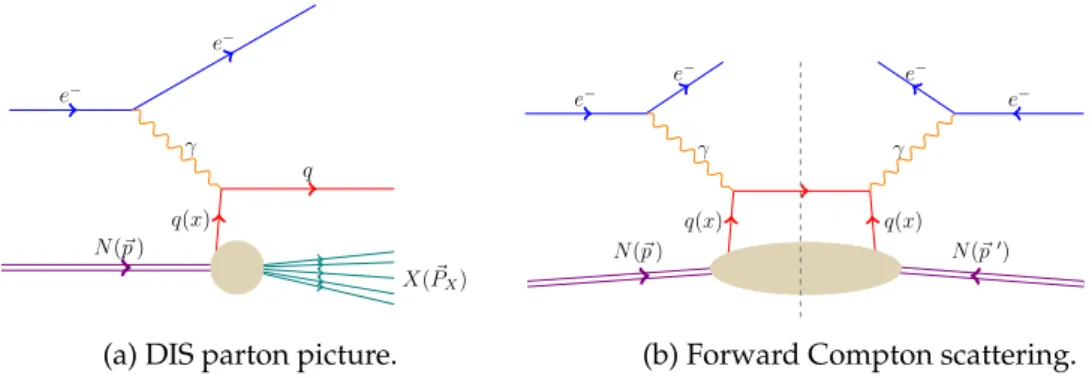
(a) DIS parton picture.

e⁻ e⁻

q(x) q(x)

γ

N(~p) N(~p⁰)

γ

e⁻ e⁻

(b) Forward Compton scattering.

Figure 2.4.: Deep inelastic scattering in the parton picture to emphasize the similarity to DVCS.

The left hand side squared after summing over all final statesX corresponds to the right hand side. The dashed line means that particles are on-shell.

deeply virtual Compton scattering by means of the optical theorem:

W^µν = 1

2πImT^µν where T^µν = i Z

d⁴ze^iq^·^zhH, λ⁰ | T {J^µ(z)J^ν(0)} |H, λi (2.6) and

W^µν = 1 4π

Z

d⁴ze^iq·zhH(p), λ⁰| J^µ(z)J^ν(0)|H(p), λi (2.7) where the polarizations of the in and out going hadrons are given byλandλ⁰ respectively and T signifies a time ordered product. Note that we have summed over all possible reaction productsXin this expression.

The leptonic tensor is known exactly, as the leptons are point-like fermions, and has a few noteworthy properties. First of all it is conserved so that

q_µl^µν =q_νl^µν = 0, (2.8)

and under µ ↔ ν the spin dependent part ofl_µν is antisymmetric, whereas the spin independent part is symmetric.

The general form of the spin ¹₂ hadronic tensor can be deduced by demanding time reversal and parity invariance and conserved currents, so that contractions withq_µand

(19)

q_ν are zero²². We find W_µν =−

g^µν−q^µq^ν q²

F₁(x_B, Q²) +F₂(x_B, Q²) p·q

p^µ−p·q

q² q^µ p^ν−p·q q² q^ν

−ig₁(x_B, Q²)

p·q ε^µνλσq_λs_h,σ− ig₂(x_B, Q²)

(p·q)² ε^µνλσq_λ(p·qs_h,σ−s_h·qp_σ) (2.9) where we denote the four-vector spin of the hadron ass_h. Now we have introduced the unpolarized structure functionsF₁andF₂and the polarized structure functionsg₁ andg2.

Underµ ↔ ν the antisymmetric part of W_µν is spin dependent and the symmetric part is spin independent, in complete analogy tol_µν. Thus to measureF₁ andF₂ it is sufficient to use an unpolarized lepton beam and an unpolarized hadron target, and to also measureg₁andg₂ both have to be polarized.

2.2.3. Operator product expansion and moments of structure functions The product of currents in Eq. (2.72.7) is non-local. Furthermore Eq. (2.72.7) is dominated by the region near the light conez² →0[1515].

With the help of the operator product expansion (OPE) one can split up the short- distance behavior, where perturbative QCD is applicable, and the long-range non- perturbative part. A general OPE for an arbitrary correlatorOiis given as

zlim²→0Oa(z)Ob(0) =X

k

c_abk(z)Ok(0). (2.10) This is generally divergent at the pointz² = 0and this divergence is encoded in the coefficient functionsc_abk. All short-scale behavior has to be treated in the coefficient functions, and in QCD short scales allow for perturbative treatment.

A concise outline of the OPE in DIS can be found in [1616]. Note that an operatorO^µ¹^···µⁿ has spinnif it is symmetrized in theµ_iand traces are subtracted. Then the contribution in the deep inelastic limit³³tol_µνW^µνof an operator with dimensiondand spinswill be of orderO(x⁻ⁿ_B

Q² mN

2+n−d

), wherem_N is the nucleon mass. In the exponent we have n−dwhich is called the negative twist, so that

twist = dimension−spin. (2.11)

The minimal twist is two and the operators of higher twist are suppressed at largeQ².

2In addition to Eq. (2.82.8) that means we could drop all terms proportional toqµ, qνinWµν, orlµν but not in both, before we contract the hadronic and leptonic tensor.

3I.e.,p·q,s·q,p·k, andp·k⁰are allO(Q²/mN).

(20)

2.2. Deep inelastic scattering The matrix elements of the operators correspond to Mellin moments of the structure functions in the decomposition of the hadronic tensorW_µν [1717].

We define then-th Mellin⁴⁴moment of a functionf as f_n=

Z∞ 0

dxxⁿ⁻¹f(x). (2.12)

There are different operators for the contributions of quarks and gluons to the structure functions. The latter will not be discussed here, but it is important to consider them as well when comparing to the experiment.

The tower of twist two operators for quarks that correspond to the structure functions which multiply Lorentz structures with the appropriate symmetries are

O^{µq ¹^µ²^...µⁿ^} = iⁿ⁻¹qγ^{µ¹D^↔^µ²· · ·D^↔^µⁿ^}q , O^{5q^µ¹^µ²^...µⁿ^} = iⁿ⁻¹qγ^{µ¹γ₅D^↔^µ²· · ·D^↔^µⁿ^}q ,

Oσq^ν^{^µ¹^...µⁿ^} = iⁿ⁻¹qσ^ν^{^µ¹γ5D^↔^µ²· · ·D^↔^µⁿ^}q , (2.13) where

D^↔_µ= 1 2

_→

Dµ−D^←µ

, (2.14)

σ_µν = i/2[γ_µ, γ_ν] and {. . .} means that indices are symmetrized and the traces subtracted.

Note that for each derivative in Eq. (2.132.13) both the spin and the dimension of the operator increase by one so that the twist is always two.

To compute then-th Mellin moment of a structure function one needs an operator with spinnand the variable with respect to which we Mellin transform is the quark momentum fractionx.

2.2.4. Parton distribution functions in the nucleon

In the parton picture the scattering photon sees only one quark in the nucleon. The computation of the individual scattering amplitudes for each quark is very analogous to a QED calculation. To break down the total cross section into the individual contributions we need to define quark densities.

In a longitudinally polarized nucleon, i.e., nucleon spin and momentum are parallel, a quark with momentum fractionxand its spin aligned with the nucleon spin has the quark densityq_↑(x, µ²)at the scaleµandq_↓(x, µ²)if its spin is opposite to the nucleon spin.

4In some sources the counting starts at zero, but we will stick to this convention.

(21)

Analogously, in a transversally polarized nucleon, i.e. nucleon spin and momentum are perpendicular, a quark with its spin aligned with the nucleon spin has the density q_⊥(x, µ²)andq_>(x, µ²)if the quark spin points in the other direction.

P~ S~

~ s

~k

q _↑

P~

S~

~s

~k

q _⊥

Figure 2.5.: Representation of quark densities, the momentum fraction of the quark is x = k+/P+. The picture should not imply that necessarily~k k P~, in fact we integrate over all~kwith a givenxto define the quark densities.

Then we define the generalized quark distribution functions⁵⁵as

q(x, µ²) =q_↑(x, µ²) +q_↓(x, µ²), (2.15)

∆q(x, µ²) =q_↑(x, µ²)−q_↓(x, µ²), (2.16) δq(x, µ²) =q_⊥(x, µ²)−q_>(x, µ²). (2.17) These functions are zero for|x|>1, and for negativexthey correspond to anti-quark distributions. We find⁶⁶[1818]

q(−x, µ²) =−q(x, µ²) (2.18)

∆q(−x, µ²) = +∆q(x, µ²) (2.19) δq(−x, µ²) =−δq(x, µ²). (2.20) Using the above we can now define a compact notation for then-th Mellin moment, that also incorporates anti-quark distributions and the constraint onx, so that we can write

˜ qn=

1

Z

−1

dxxⁿ⁻¹q(x)˜ , (2.21)

forq˜∈ {q,∆q, δq}.

With these definitions we can re-express the structure functions by the individual con-

5Alternativelyf1≡q,g1≡∆q, andh1≡δqare found in the literature.

6This can be seen by using the charge conjugation properties of the corresponding quark bilinears defined in Eq. (2.242.24).

(22)

2.3. Moments of GPDs

tributions of each quark flavor. In the unpolarized case one finds F1(xB, Q²) = 1

2x_BF2(xB, Q²) = 1 2

X

q

c²_el.,q q(xB, Q²) +q(xB, Q²)

, (2.22) where the respective electrical charge of each quark flavor in units of the electron charge is denoted byc_el.,q ∈₋₁

3 ,²₃ and it is customary to set the scaleµ² =Q² and to lowest order⁷⁷x=x_B. The proportionality ofF₁andF₂is a consequence of the quarks having spin ¹₂ and this was used to experimentally justify this picture. Bjorken scaling [1919] is reached at highQ² when in Eq. (2.222.22) theF_i become independent ofQ². It was a good description of the older DIS data and at the same time it was clear that such scaling would be violated. Mild scaling violations could only be explained in an asymptotically free theory.

In a manner similar to Eq. (2.222.22) the polarized structure functiong₁is g₁(x_B, Q²) = 1

2 X

q

c²_el.,q ∆q(x_B, Q²) + ∆q(x_B, Q²)

. (2.23)

Note that the transversal quark density δq does only appear in processes that have a helicity-flip [2020], e.g., some channels in semi-inclusive DIS, and it is thus inherently more difficult to measure than the other two quark density combinations. See [2121] for a recent review.

2.3. Moments of GPDs

In the previous section we have parameterized the time-ordered product of two electromagnetic currents in between two nucleon states by the structure functions and in the parton picture we have then broken them down to the parton distribution functions. To generalize this case to the non-forward scattering we need to replace the two currents by Fourier transformed bilocal operators, which depend on the momentum fraction of the quarkx, of the form⁸⁸[2222]

O_Γ^q(x) = Z _∞

−∞

dα 2πe^iαxq

−α 2n

ΓU[−^α₂n,^α₂n]qα 2n

, (2.24)

7In Eq. (2.72.7) the exponent is an oscillating phase. The integrand contributes most if the longitudinally probed distance, also called Ioffe time,z⁻≈(M xB)⁻¹. The momentum associated to this distance is the quark momentum fractionx, thusx≈xB. See Section 2.2.4 of [1010] for a more thorough explanation.

8Note that in the conventions of [2222]nis a light cone vector withP·n= 1.

(23)

where the Wilson line

U[−^α₂n,^α₂n]=Pe^ig

R₋α/2

α/2 dλ n·A(λn) (2.25)

is a path ordered (denoted by P) exponential of gauge fields and it ensures gauge invariance.

The matrix elements of this bilocal operators are then decomposed into different Lorentz structures and the scalar prefactors are the GPDs. In the DIS discussion, Section 2.22.2, these prefactors of the Lorentz structures were the structure functions after we expressed them through the PDFs. The Lorentz structures depend on theΓ we use in Eq. (2.242.24). Possible independent twist two operators areO_V,O_A, andO_T whereΓwas chosen asγµ,γ5γµandiσµν respectively.

The GPDs depend on the momentum transferQ² =tand we have to renormalize them at a scaleµ. In the DIS case we setµ² =Q², a choice which is not suitable to study the Q²-dependence of GPDs. To avoid confusion we will write them as functions oftand suppress the scale dependence for now. The list of GPDs [2222] is

hN(p⁰)|O_V^µ(x)|N(p)i=U(p⁰)

γ^µH(x, ξ, t) +iσ^µν∆_ν

2m_N E(x, ξ, t)

U(p), (2.26) hN(p⁰)|O_A^µ(x)|N(p)i=U(p⁰)

γ^µγ5H(x, ξ, t) +e γ₅∆^µ

2m_NE(x, ξ, t)e

U(p), (2.27) hN(p⁰)|O_T^µν(x)|N(p)i=U(p⁰)

(

iσ^µνH_T(x, ξ, t) +γ^[µ∆^ν]

2m_N E_T(x, ξ, t) + P^[µ∆^ν]

m²_N He_T(x, ξ, t) +γ^[µP^ν]

m_N Ee_T(x, ξ, t) )

U(p), (2.28) where we omitted contributions of higher twist.

With the help of the OPE we can express these matrix elements of bilocal operators as expansionw in matrix elements of the local operators defined in Eq. (2.132.13), the moments of the GPDs of generalized form factors GFFs. A systematic expression of the moments of GPDs and the decomposition in the matrix elements can be found in [2323].

In this work we only present the lowest moments and we will state them in Section 2.42.4.

The connection between the GPDs and the quark densities defined earlier is given by considering the forward case:

q(x) =H(x,0,0), (2.29)

∆q(x) =H(x,e 0,0), (2.30)

δq(x) =H_T(x,0,0). (2.31)

(24)

2.4. Lowest moments of GPDs, form factors and charges

To illustrate the GPDs we can consider impact parameter distributions like H(x,b) =

Z d²∆

(2π)²e⁻^ib∆H(x,0,−∆²), (2.32) at zero skewness. The transverse momentum transfer∆and impact parameterblive in the 2d-transverse plane⁹⁹. Similar transformations can be done for the other GPDs.

Doing this for a linear combination of Eq. (2.262.26) and Eq. (2.282.28) we obtain the density of quarks with transverse polarization¹⁰¹⁰:

1 2

F+sⁱF_Tⁱ

(x,b) = 1 2

hH(x,b)−bsinϕ 1 m_N

∂

∂b²E(x,b)

−bsin(ϕ−χ) 1 mN

∂

∂b² (E_T(x,b) + 2H_T(x,b)) + cosχ

H_T(x,b)− 1 m²_N

∂

∂b² b² ∂

∂b²H˜_T(x,b)

+b²cos(χ−2ϕ) 1 m²_N

∂

∂b² 2

H˜_T(x,b)i

(2.33) where we assume the nucleon spinS = (1,0)and the quark spins= (cosχ,sinχ), and we writeb=b(sinϕ,cosϕ)withb=√

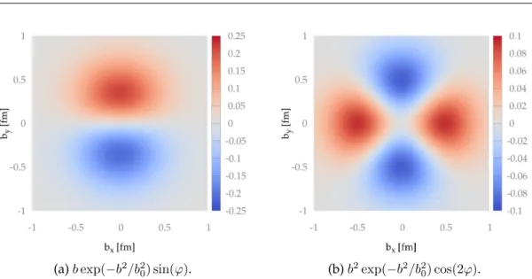
b². We can identify structures which break rotational symmetry and through them we can extract the angle of the quark spinχto the nucleon spin. When additionally assuming ab²-dependence of the parton distributions asexp(−b²/b²₀)withb₀ = 0.5fm these can then be plotted in theb_x-by plane, as shown in Fig. 2.62.6or [2424].

2.4. Lowest moments of GPDs, form factors and charges

In this section we will present the matrix elements of local operators that we can compute in lattice QCD and their physical significance. We use the abbreviation

hhOii=U(P⁰, σ⁰)O U(P, σ), (2.34) in the following.

We present a subjective selection of the properties of the matrix elements and do not claim to present a complete review of these quantities. Gluonic contributions are matrix elements of field strength tensors with appropriateγ-matrices and derivatives [1111]. We will focus on the contributions of quarks to the GPDs for most part.

9We will denote vectors in this plane by bold symbols.

10We use the notion of [2424] and do not give the left hand side a new name.

(25)

(a)bexp(−b²/b²₀) sin(ϕ). (b)b²exp(−b²/b²₀) cos(2ϕ).

Figure 2.6.: Rotational invariance breaking contributions to the transverse quark density in the bx-byplane. The color scale is arbitrary and the plot design is taken from [2424].

2.4.1. Scalar form factor

The scalar form factor is actually a matrix element of a twist three operator. Thus it has no relation to our twist two GPDs, but is mentioned here for completeness because the techniques to compute it are the same as for the moments of GPDs.

The matrix element is

hP⁰ |Ψ_qΨ_q |Pi=hh1iiG_S(t). (2.35) It signifies the coupling of the nucleon to scalar particles, like the Higgs-boson and it is relevant also in some extensions of the standard model [2525].

At zero recoil (p=p⁰= 0) the scalar matrix element is related to the sigma terms

σq =mqhN |qq |Ni. (2.36)

The pion nucleon sigma termσ_πN =σu+σ_dplays an important role as a low energy constant for chiral perturbation theory.

As it is an iso-scalar quantity, disconnected contributions to the three-point function cannot be neglected. It contains a unit matrix as choice ofΓin Eq. (2.242.24). Hence it is the simplest quantity for which quark line disconnected diagrams are required. Therefore many lattice studies exist [2626] on this topic and it is an ideal playground to test signal- to-noise improvement strategies for disconnected diagrams.

An alternative scheme to compute the relevant matrix elements is given by the Feyn-

(26)

man-Hellman theorem

σ_q =m_q∂M_N

∂m_q . (2.37)

It was used in lattice studies like [2727], and so one can cross-check the simulations on the lattice.

Theσ-term can be used to constrainm_N(m_q)and thus aid in the extrapolation of lattice results to physical quark masses. This was used in [2828, 2929] to determine r₀m_N and hencer₀in physical units. Alternatively it can serve as a benchmark of the scale setting as outlined in [3030].

2.4.2. Dirac and Pauli form factors

The electromagnetic form factors can be obtained from hP⁰ |Ψ_qγ^µΨ_q|Pi=hhγ^µiiF₁^q(t) + i

2m_N

σ_M^µν

∆_νF₂^q(t). (2.38) The relation to GPDs is given by

F₁^q(t) = Z 1

−1

dx H^q(x, ξ, t), F₂^q(t) = Z 1

−1

dx E^q(x, ξ, t). (2.39) The electromagnetic current, where we again define electric charges in units of the ele- mentary chargee, is given by

J_e/m^µ = 2

3uγ^µu−1

3dγ^µd , (2.40)

and thus the Dirac form factorF₁(no spin flip) and the Pauli form factorF₂(spin flip) for the proton (when the nucleon in Eq. (2.382.38) is taken as a proton ) are the linear combinations of

F_1/2(t) = 2

3F_1/2^u (t)−1

3F_1/2^d (t). (2.41)

In the limit oft→ 0they yield, after renormalization, the electric charge of the proton gV = F1(0) = 1 andF2(0) = µp −1 where µp = 2.7928 is the magnetic moment of the proton. Note that the vector couplingg_V corresponds to a conserved current and thus transition matrix elements would be zero. This means that on the lattice we expect to get flat plateaus. Excited state contributions could be present, but they would be suppressed bye⁻^∆mt^sink, see Section 5.15.1.

A point particle would have t-independent form factors, so a non-trivial momentum

(27)

transfer dependence allows for insights on the structure of the nucleon like the spatial charge distribution. Lattice studies include [3131].

The Dirac radiusr₁and the Pauli radiusr₂of the proton can indeed be computed from F₁/F2via

hr_i²i=−6dFi

dQ² |Q²=0, i= 1,2. (2.42)

The linear combinations

G_E(t) =F₁(t)− t

(2m_N)²F₂(t) (2.43)

G_M(t) =F₁(t) +F₂(t), (2.44) are the electric and magnetic Sachs form factors. The corresponding radii, computed in complete analogy to Eq. (2.422.42), are the magnetic and charge radius of the nucleon.

For the charge radius two contradicting experimental results [3232] exist and there is an ongoing discussion in the literature [3333]. Current lattice studies like [3434] fail to resolve the discrepancy between them. In [3434] the difference to the experimental results is attributed to the presence of excited state contributions.

In the iso-spin symmetric limit we have the identity [3535]

J_e/m;u−d^µ =uγ^µu−dγ^µd . (2.46)

This current has the advantage that disconnected contributions for the light flavors cancel in this limit.

Another choice often found in the literature is the iso-scalar (is) form factor. For these two combinations of flavors we define

F_1/2îv (t) =F_1/2û (t)−F_1/2^d (t), F_1/2îs (t) =F_1/2û (t) +F_1/2^d (t). (2.47) 2.4.3. Axial form factors

From the axial current we obtain

hP⁰|Ψqγ^µγ5Ψq|Pi=hhγ^µγ5iiG^q_A(t) + ∆^µ

2m_N hhγ5iiG^q_P(t), (2.48)

(28)

whereG^q_A(t)is the axial form factor andG^q_P(t)is the induced pseudoscalar form factor.

The axial coupling of the nucleon, which also parameterizes the strength ofβ-decay, is g_A=G^u_A(0)−G^d_A(0).

In this combination the disconnected contributions to the matrix element cancel in the iso-spin limit. This simplifies the computation significantly and thus this quantity has been studied extensively on the lattice, see Section 4.14.1for a review on recent results.

The pseudoscalar coupling constant is connected to the axial coupling [3636] via the Goldberger-Treiman [3737] relation, using PCAC,

mµ

2m_NG^u_P⁻^d(t)≡g_P(t) = 2mµmN

m²_π+t (2.49)

This is a first order result and it can be compared to the experiment to test the accuracy of the PCAC prediction. For a recent review see [3838].

The threshold for muon capture of the proton is t = 0.88m²_µ and hence one usually quotesg_P =g_P(0.88m²_µ). From Eq. (2.492.49) one would expectg_P ≈6.77g_A.

The GFFs of Eq. (2.482.48) are the first moments ofHe andE:e GA(t) =

Z 1

−1

dxH(x, ξ, t)e , GP(t) = Z 1

−1

dxE(x, ξ, t)e . (2.50) By looking at the definition of the quark densities Eq. (2.162.16), using Eq. (2.302.30) and Eq. (2.502.50) we find

g_A= Z 1

−1

dx (∆u(x)−∆d(x)), (2.51)

which is the net-contribution to the longitudinally polarized spin of the proton by the up-quarks minus the down-quark contributions.

The proton spin crisis was initiated by the EMC [99] experiment measuring that the quark spin contributions are small and cannot account for the proton spin alone. The individual contributions of the partons to the hadron spin can be split up like this [1111]

J = 1

2∆Σ +L_q+J_G. (2.52)

The orbital angular momentum terms of quarks isL_q and the total gluon spin contribution J_G. To compute them one needs also disconnected contributions and gluonic operator insertions. This was, e.g., done in [3939].

(29)

The total quark spin contributions can be summed up¹¹¹¹

∆Σ = ∆u+ ∆d+ ∆s+ ∆u+ ∆d+ ∆s . (2.53) The light quark part of the spin can be computed from the matrix elements of Eq. (2.482.48), where one also needs the disconnected diagrams.

The strange quark contributions to the nucleon spin stem from disconnected contributions to three-point functions. They can be evaluated in LQCD with the help of all-to-all propagators. This is e.g. done by the Regensburg group [4040].

It is an ongoing debate whether one can define the individual contributions to the nucleon spin as [4141]

J = 1

2∆Σ + ˜Lq+LG+ ∆G , (2.54) in a gauge invariant way. As way to organize computations of∆Git was suggested to split the gauge potential up in contributing and non-contributing parts in, e.g., [4242], but the solution is not unique [4343]. For an extensive overview article in this c.f. [4444].

In [4545] it is argued that the difference between the quark orbital angular momentumL_q in Eq. (2.522.52) andL˜qin Eq. (2.542.54) is due to final state interactions, after the quark has left the target in a deep inelastic scattering.

2.4.4. Tensor form factors

The tensor current with no derivatives yields

hP⁰ |Ψ_qiσ^µνΨ_q|Pi=hhiσ^µνiiA_T₁₀(t) +DD

γ^[µ∆^ν]EEB_T₁₀(t) 2m_N +hh1iiP^[µ∆^ν]A˜_T₁₀(t)

m²_N . (2.55)

The form factors are the first moments of the tensorial GPDs:

A_T₁₀(t) = Z ₁

−1

dxH_T(x, ξ, t), B_T₁₀(t) = Z ₁

−1

dxE_T(x, ξ, t), Ae_T₁₀(t) =

Z 1

−1

dxHe_T(x, ξ, t). (2.56) The first moment of Ee_T(x, ξ, t) vanishes hence there are only three generalized form factors in Eq. (2.552.55), whereas there are four GPDs in the matrix element of the bilocal tensor operator Eq. (2.282.28).

11We neglect heavier sea quark flavors and imply∆q=R1

0 ∆q(x)dx.

(30)

2.4. Lowest moments of GPDs, form factors and charges The tensor couplingg_T =A^u−d_T₁₀(t)is similar tog_Aas it is given (see Eq. (2.172.17), Eq. (2.312.31)) as

g_T = Z 1

−1

dx δu(x)−δd(x). (2.57)

The non-relativistic quark model predicts ∆u = δu = ⁴₃ and ∆d = δd = −¹₃, viz g_A=g_T.

Lorentz-boosts in a relativistic theory single out the boost direction and thus break the rotational invariance of the proton, and introduce antiparticle contributions. Thus the difference of axial coupling and tensor coupling is a measure of these relativistic effects.

The tensor coupling is experimentally much harder to access than g_A as it cannot be measured in DIS. The transverse spin structure can only be probed in processes with a helicity flip of the struck quark.

Experimental extractions ofgT also use the Soffer bound [4646]

q(x) + ∆q(x)≥2|δq(x)|, (2.58) to constrain their fits.

For a recent lattice result see [4747].

2.4.5. Second moment of vector GPDs

The second moments of GPDs are generally obtained by matrix elements of operators with one derivative. In the vector current case this yields

hP⁰ |Ψ_qγ^{^µD^↔^ν^}Ψ_q|Pi=S(µ, ν)

hhγ^µiiP^νA₂₀(t) +hhiσ^µαii∆_αP^ν

2m_N B₂₀(t) +hh1ii∆^µ∆^ν

m_N C₂₀(t)

. (2.59) Here we have to subtract the traces on both sides, see Appendix C.2.1C.2.1. The indicesµ, ν are symmetrized on both sides, indicated by the symmetrization function S(µ, ν) and the curly brackets on the left side.

The first moments of the vector GPDs correspond to these linear combinations of GFFs:

Z 1

−1

dxxH(x, ξ, t) =A₂₀(t) + (2ξ)²C₂₀(t), Z 1

−1

dxxE(x, ξ, t) =B₂₀(t)−(2ξ)²C₂₀(t). (2.60)