2 Stochastic baryonic and mesonic three-point correlation functions

(1)

Baryonic and mesonic 3-point functions with open spin indices

Gunnar S. Bali¹^,², Sara Collins¹, Benjamin Gläßle¹, Simon Heybrock³, Piotr Korcyl¹^,⁴, Marius Löffler¹^,,RudolfRödl¹, andAndreasSchäfer¹

1Institut für Theoretische Physik, Universität Regensburg, D-93040 Regensburg, Germany

2Department of Theoretical Physics, Tata Institute of Fundamental Research, Homi Bhabha Road, Mumbai 400005, India

3European Spallation Source, 225 92 Lund, Sweden

4M. Smoluchowski Institute of Physics, Jagiellonian University, ul. Łojasiewicza 11, 30-348 Kraków, Poland

Abstract.We have implemented a new way of computing three-point correlation functions. It is based on a factorization of the entire correlation function into two parts which are evaluated with open spin- (and to some extent flavor-) indices. This allows us to estimate the two contributions simultaneously for many different initial and final states and momenta, with little computational overhead. We explain this factorization as well as its efficient implementation in a new library which has been written to provide the necessary functionality on modern parallel architectures and on CPUs, including Intel’s Xeon Phi series.

1 Introduction

Observables constructed with the use of three-point correlation functions can describe a multitude of physical phenomena, such as the parton structure of hadrons or their weak transitions, depending on the operator type at the insertion. The relevant strong interaction matrix elements can be computed using Lattice Quantum Chromodynamics. Traditionally, a method employed to that aim was the sequential source method [1]. The numerical cost of this is high because a new inversion is necessary for each final momentum at the sink. In this contribution we present a stochastic algorithm which circumvents this limitation and disentangles the number of inversions of the lattice Dirac operator from the number of sink/insertion momenta. The implementation we propose parallelizes the computations in such a way that multiple source positions and multiple insertion positions can be estimated simultaneously. Moreover, by storing the uncontracted data, with all spin indices open, on disk, we enable the user to analyse any channel of interest at a later stage.

An aspect of our implementation which we wish to highlight in this contribution is the extensive use of vectorization. As the compute power of today’s processors relies on longer and longer vector registers of additional vector processing units, an adequate data layout is required to efficiently use these resources. We explain our data layout which supports large vector registers, therefore en- abling us to efficiently run our code on the Intel’s Xeon Phi processors featuring 512 bit AVX vector instructions.

Speaker, e-mail: marius.loeffler@physik.uni-regensburg.de

(2)

Our implementation is based on a framework developed specifically for Intel’s Xeon Phi processors, calledLibHadronAnalysissee, e.g., [2,3]. This library contains additional routines for computing meson and baryon spectra, meson and baryon distribution amplitudes and many other objects.

Compared to a naive implementation in Chroma [4] using QDP++[4] objects it provides speed-up factors of the order 10-20 on the KNC and KNL architectures.

Below we describe in detail the algorithm. In particular we explain how the computation of a three- point correlation function can be separated into two, largely independent parts, the “spectator” and the

“insertion” parts. We pay special attention to the parallelization schemes which are different for each of these parts. Subsequently, we present benchmarks showing the performance of our implementation on a KNL cluster, and then we conclude.

2 Stochastic baryonic and mesonic three-point correlation functions

In this section we introduce the three-point correlation function we are interested in and show how it can be factorized into two, largely independent parts. We only show explicit formulae for the case of meson three-point functions, for the sake of notational simplicity. A similar approach was used in Refs. [5–8], however, here we keep all spin indices open.

2.1 General structure

A three-point meson correlation function (c.f., figure1) with a sourceC(r), a sinkA(x) and an insertion operatorI(y), located at timeslicesr4,x₄andy₄respectively, reads

A(x)I(y)C(r)=tr

Gf1(r,x)Γ_snkGf2(x, y)Γ_ins Gf3(y,r)Γ_src

= δab δab δa˜_˜b Γ^α_snk^β Γ^α˜_ins^˜^β Γ^βα_src Gf1(r,x)^αα_aa Gf2(x, y)^β_b^αa^˜˜ Gf3(y,r)^ββ_˜_bb^˜ (1) where

A(x,x₄)=δab ψ_f₂(x,x₄)^α_a Γ^α_snk^β ψf1(x,x₄)^β_b , (2) C(r,r₄)=δba ψ_f₁(r,r₄)^β_b

γ₄Γ^†γ₄βα

ψf3(r,r₄)^α_a , (3)

I(y, y4)=δ_a_˜b˜ ψ_f₃(y, y4)^α_a_˜^˜ Γ^α˜_ins^˜^β ψf2(y, y4)^β_b^˜_˜ , (4) are the annihilation, creation and insertion operators respectively, with fi ∈ {l,s,c}(light, strange, charm). Gfi(r,x) is a standard fermion propagator from xtorof flavor fi. We use the convention to denote the annihilation spin and color operator indices with primed Greek and Latin lettersα,a, creation operator indices with ordinary Greek and Latin lettersα,a, and the insertion operator indices with tilde Greek and Latin letters ˜α,a.˜ Γ_ins can contain local derivatives andAandC may contain quark smearing.

At this point we replace one of the propagators by its stochastic estimate

Gf₂(y,x)^αβ_ab^˜_˜ ≈ 1 N

N

i=1

si,f₂(y)^α_a_˜^˜ η^∗_i(x)^β_b , (5)

(3)

Our implementation is based on a framework developed specifically for Intel’s Xeon Phi processors, calledLibHadronAnalysissee, e.g., [2,3]. This library contains additional routines for computing meson and baryon spectra, meson and baryon distribution amplitudes and many other objects.

Compared to a naive implementation in Chroma [4] using QDP++[4] objects it provides speed-up factors of the order 10-20 on the KNC and KNL architectures.

Below we describe in detail the algorithm. In particular we explain how the computation of a three- point correlation function can be separated into two, largely independent parts, the “spectator” and the

“insertion” parts. We pay special attention to the parallelization schemes which are different for each of these parts. Subsequently, we present benchmarks showing the performance of our implementation on a KNL cluster, and then we conclude.

2 Stochastic baryonic and mesonic three-point correlation functions

In this section we introduce the three-point correlation function we are interested in and show how it can be factorized into two, largely independent parts. We only show explicit formulae for the case of meson three-point functions, for the sake of notational simplicity. A similar approach was used in Refs. [5–8], however, here we keep all spin indices open.

2.1 General structure

A three-point meson correlation function (c.f., figure1) with a sourceC(r), a sinkA(x) and an insertion operatorI(y), located at timeslicesr4,x₄andy₄respectively, reads

A(x)I(y)C(r)=tr

Gf1(r,x)Γ_snkGf2(x, y)Γ_insGf3(y,r)Γ_src

= δab δab δ_a_˜b˜ Γ^α_snk^β Γ^α_ins^˜^β^˜ Γ^βα_src Gf1(r,x)^αα_aaGf2(x, y)^β_b^αa^˜˜ Gf3(y,r)^ββ_bb^˜_˜ (1) where

A(x,x₄)=δab ψ_f₂(x,x₄)^α_a Γ^α_snk^β ψf1(x,x₄)^β_b , (2) C(r,r₄)=δba ψ_f₁(r,r₄)^β_b

γ₄Γ^†γ₄βα

ψf3(r,r₄)^α_a , (3)

I(y, y4)=δ_˜a˜b ψ_f₃(y, y4)^α_˜_a^˜ Γ^α˜_ins^˜^β ψf2(y, y4)^β_b_˜^˜ , (4) are the annihilation, creation and insertion operators respectively, with fi ∈ {l,s,c}(light, strange, charm). Gfi(r,x) is a standard fermion propagator from xtorof flavor fi. We use the convention to denote the annihilation spin and color operator indices with primed Greek and Latin lettersα,a, creation operator indices with ordinary Greek and Latin lettersα,a, and the insertion operator indices with tilde Greek and Latin letters ˜α,a.˜ Γ_ins can contain local derivatives andAandC may contain quark smearing.

At this point we replace one of the propagators by its stochastic estimate

Gf₂(y,x)^αβ_ab_˜^˜≈ 1 N

N

i=1

si,f₂(y)^α_a^˜_˜ η^∗_i(x)^β_b , (5)

where the sum runs overNrealizations of the noise source vectorηi(x), with the properties 1

N

i=1

(ηi) (x)^α_a =0+O

1

√N

, (6)

1 N

N

i=1

(ηi) (x)^α_a

η^∗_i(x)^α_a=δxx δαα δaa+O

1

√N

. (7)

The (ηi) (x) are time partitioned and set to zero, unlessx4=x₄orx4=x₄.

r4

x₄ y4

τ x₄

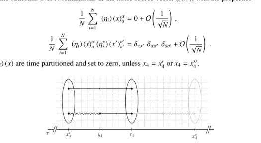
Figure 1.Sketch of the structure of a generic three-point correlation function.

In figure1we show the generic structure of a three-point correlation function in the meson case.

The central ellipse denotes a meson created with operator Eq. (3) in the middle of the lattice at times- licer₄. The meson is annihilated by the operator from Eq. (2) at the timeslicex₄ as depicted by the left-most ellipse. Arrows denote exact point-to-all propagators. The star at timeslicey₄denotes one of the possible positions of the insertion operator. The wiggly line is used to plot the stochastic all-to-all propagator. We call these four elements the “forward” correlation function as opposed to the shaded mirror-reflected graph on the right hand side which corresponds to the “backward” process. The forward and backward diagrams are estimated simultaneously which allows for increased statistics.

The introduction of the stochastic propagator allows us to factorize the correlation function A(x)I(y)C(r)into two parts [5] as follows

A(x)I(y)C(r)= δab δab δa˜_˜b Γ^α_snk^β Γ^α˜_ins^˜^β Γ^βα_src ×

×

γ₅ G^†_f₁(x,r)γ₅αα aa

ηi(x)γ₅β b

=ˆSpectator

γ₅ si,f₂(y)∗α˜

˜

a Gf₃(y,r)^ββ_˜_bb^˜

=ˆInsertion

(8)

We define the spectatorSi,f1(p,x₄)a^β^α^αand the insertionIi,f2,f3(q, y4)^αa^˜^{β β}^˜ parts Si,f₁(p,x₄)^βa^α^α=

x

δab

ηi(x)γ5β b

γ5G^†_f₁(x,r)γ5αα

aa ·e⁻ⁱ^p^·x , (9)

Ii,f2,f3(q, y4)^αa^˜^{β β}^˜ =

y

δab δa˜_˜b

γ₅ si,f2(y)_∗α˜

˜

a Gf3(y,r)^ββ_bb_˜^˜ ·eⁱ^q·y , (10) where we have assumedr=0. Otherwise we have to replacex→x−r, y→y−r.

2.2 Spectator part

The computation of the spectator part consists of the contractions of propagators at the timeslices where the source and the sink are located. Naively only the MPI ranks working on the timeslicesr4

(4)

andx₄,x₄ would work. In our implementation we prepare a set of propagators sourced from different temporal source positions, as shown on figure2. We redistribute these propagators among the different MPI ranks in such a way that each rank has at least one propagator. The computation of the spectator part for each source position is than performed simultaneously. The Fourier transformation Eq. (9) fixes the momentumpat the sink.

x₄ x₄

τ r41 r42 r43 r44

Figure 2. Parallelization of the spectator part of the three-point correlation function. Propagators sourced at different timeslices denoted by different solid ellipses are redistributed among all MPI ranks so that each rank has at least one set of propagators to work with.

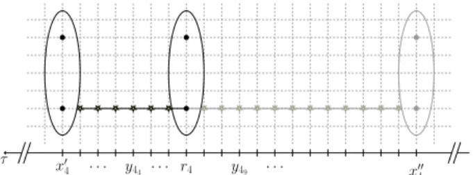
2.3 Insertion part

The insertion part corresponds to the contraction of the stochastic propagator, i.e., the solution of the lattice Dirac equation sourced by random noise vectors, with the point-to-all propagator. This has to be repeated for each positiony₄of the insertion operator between the sinksx₄andx₄and the sourcer₄. Again, in order to keep a good workload balance we redistribute the data from the timeslices where the insertion is present, denoted with stars on figure3, among all MPI ranks in such a way that each rank has approximately the same number of insertion positions to work with, and we perform all the computations in parallel. Note that a separate Fourier transformation in Eq. (10) allows to select a desired momentumqflowing through the insertion.

x₄

τ · · · y44 · · · r4 y49 · · · x₄

Figure 3.Parallelization of the insertion part of the three-point correlation function. Data from timeslices denoted with yellow stars is redistributed among all MPI ranks, such that all ranks have a similar workload.

3 Performance

We paid special attention to the data layout to enable the use of vectorization. The crutial point was to reorder the many loops in the algorithm. We show this explicitly for pseudocode in listings1and2.

(5)

andx₄,x₄ would work. In our implementation we prepare a set of propagators sourced from different temporal source positions, as shown on figure2. We redistribute these propagators among the different MPI ranks in such a way that each rank has at least one propagator. The computation of the spectator part for each source position is than performed simultaneously. The Fourier transformation Eq. (9) fixes the momentumpat the sink.

x₄ x₄

τ r41 r42 r43 r44

Figure 2. Parallelization of the spectator part of the three-point correlation function. Propagators sourced at different timeslices denoted by different solid ellipses are redistributed among all MPI ranks so that each rank has at least one set of propagators to work with.

2.3 Insertion part

The insertion part corresponds to the contraction of the stochastic propagator, i.e., the solution of the lattice Dirac equation sourced by random noise vectors, with the point-to-all propagator. This has to be repeated for each positiony₄of the insertion operator between the sinksx₄andx₄and the sourcer₄. Again, in order to keep a good workload balance we redistribute the data from the timeslices where the insertion is present, denoted with stars on figure3, among all MPI ranks in such a way that each rank has approximately the same number of insertion positions to work with, and we perform all the computations in parallel. Note that a separate Fourier transformation in Eq. (10) allows to select a desired momentumqflowing through the insertion.

x₄

τ · · · y44 · · · r4 y49 · · · x₄

Figure 3.Parallelization of the insertion part of the three-point correlation function. Data from timeslices denoted with yellow stars is redistributed among all MPI ranks, such that all ranks have a similar workload.

3 Performance

We paid special attention to the data layout to enable the use of vectorization. The crutial point was to reorder the many loops in the algorithm. We show this explicitly for pseudocode in listings1and2.

for3 spin indicesdo forcolor indices a,bdo

forall sites in the local latticedo

end end end

Algorithm 1:Reference implementation

forall sites in the local latticedo for1 spin indexdo

forcolor indices a,bdo for2 spin indices SIMD vect.do end

end end end

Algorithm 2:LHA implementation

Benchmarks were performed on the QPACE3 supercomputer of the SFB/TR 55 at the Jülich Su- percomputing Centre. The machine is based on Intel Xeon Phi (KNL) processors connected via Intel Omni-Path. We used the Intel compiler version 17.0.2.

The LibHadronAnalysis library [2] was incorporated into the QDP++/Chroma software stack [4], together with the multigrid solver [9–13] optimized for the KNL architecture.

The computations were carried out on a single configuration of the CLS ensemble H101 [14].

It is aNf =2+1 ensemble with non-perturbativelyO(a) improved Wilson fermions and tree-level improved Symanzik gauge action and features open boundary conditions in time. The pion and kaon masses are about 420 MeV and this 32³×96 lattice has a lattice spacing of about 0.086 fm.

Actual measurements were performed for the meson spectator part Eq. (9) and insertion part Eq. (10) using r4 = 30a and a source-sink separation of r4−x₄ = x₄ −r4 = 10a. Within the spectator part propagators are smeared at the source and the sink time-slice while in the insertion part only the source time-slice of the propagator is smeared. The number of stochastic indices is set to Ni=50.

Running on 4−32 KNLs and distributing the 256 hardware threads on each KNL to 8 MPI tasks yields the strong scaling for the meson spectator and insertion part contraction as shown in figure4.

Note that the computation is done for 50 independently seeded stochastic estimators in forward and backward direction, i.e., the mean values are averaged over 100 computations each. The creation times for the noise and the solution vectors are not considered.

For the spectator/insertion a minimal computation time is achieved using 8/32 KNLs with 8 tasks per node. In this setup the Intel Omni-Path connection between the nodes becomes saturated, the computation is well parallelized and the overhead due to internal communication is not dominant.

In addition the wallclock-time for a particular measurement using two different ranges of momenta on one H101 configuration is evaluated – again 8 KNLs with 8 tasks per node are used. The timings fork =k² =0 and fork,k² =0, . . . ,8 for spectator and insertion momenta are shown in figure5, wherep_i = k_i2π/L,qi = ki2π/Lwhere the integersk_i andki label the momentum components of pandqwithin the Fourier transformation. Note that in these timings also a baryon measurement is included. In both cases the overall computation time is almost the same

LibHadronAnalysiswallclock-time fork²=k²=0:≈530s

LibHadronAnalysiswallclock-time fork²,k²=0, . . . ,8 (93·93 mom. combinations):≈575s.

Hence it is possible to produce data for a large number of final momenta without increasing the computation time significantly. In addition the data-layout presented in Eq. (9) and Eq. (10) provides analysis capabilities for various physical channels since theΓ-structures of the source and sink interpolators are not specified during the simulations.

Thek²,k² =0, . . . ,8 measurement was also performed using the sequential source method [1]

which yields a run-time of≈930s. Compared to the above wallclock-time of≈575s this is a speed-up of≈1.6 where we have not taken into account that the stochastic code gives 16·16Γ-combinations at

(6)

source and sink for free. First tests have shown that the computation time of the analysis code needed to obtain final three-point function results is in the range of a few seconds and therefore is negligible.

Collectively this means that one needs≈82 KNL core hours to perform the above measurement on a single configuration of the H101 assuming that 8 nodes with 64 cores per node are used. Altogether 2016 configurations are available to analyse the H101, i.e., at most≈ 165000 KNL core hours are needed to analyze the entire ensemble for every combination of source and sink meson and baryon interpolators on a single source time slice and for the given source sink separation∆t=10a. Due to the distribution shown in figure5the overall computation time should remain almost constant when increasing the number of source positions, always provided that the computation of the spectator part can be fully parallelized.

0 4 8 16 32

0 0.2 0.4 0.6 0.8 1

KNL Nodes (Wallclock-time)−1inms−1

Meson spectator

0 4 8 16 32

0 0.05 0.1 0.15

Insertion

Figure 4.Strong scaling for the spectator (left) and the insertion (right) parts for the meson three-point correlation function. Measurements were done on a 32³×96 lattice, withk² =k²=0 and 100 stochastic estimates for the stochastic propagators.

Contraction Part (0.275 %) Gauge Field (4.279 %) Source calc.

(1.890 %) Propagator calc.

(15.185 %) Solutions calc.

(71.54 %) Noises calc.

(0.562 %) Overhead (6.267 %) Contraction

Figure 5. Contribution of the contraction time to the total time budget of the three-point correlation function estimation. On the left panel the case of total momentum 0 is shown, whereas on the right panel the spectator and insertion momentum square of 0, . . . ,8 (i.e., 93·93 momentum combinations) is shown.

(7)

source and sink for free. First tests have shown that the computation time of the analysis code needed to obtain final three-point function results is in the range of a few seconds and therefore is negligible.

Collectively this means that one needs≈82 KNL core hours to perform the above measurement on a single configuration of the H101 assuming that 8 nodes with 64 cores per node are used. Altogether 2016 configurations are available to analyse the H101, i.e., at most≈ 165000 KNL core hours are needed to analyze the entire ensemble for every combination of source and sink meson and baryon interpolators on a single source time slice and for the given source sink separation∆t=10a. Due to the distribution shown in figure5the overall computation time should remain almost constant when increasing the number of source positions, always provided that the computation of the spectator part can be fully parallelized.

0 4 8 16 32

0 0.2 0.4 0.6 0.8 1

Meson spectator

0 4 8 16 32

0 0.05 0.1 0.15

Insertion

Figure 4.Strong scaling for the spectator (left) and the insertion (right) parts for the meson three-point correlation function. Measurements were done on a 32³×96 lattice, withk²=k²=0 and 100 stochastic estimates for the stochastic propagators.

Figure 5. Contribution of the contraction time to the total time budget of the three-point correlation function estimation. On the left panel the case of total momentum 0 is shown, whereas on the right panel the spectator and insertion momentum square of 0, . . . ,8 (i.e., 93·93 momentum combinations) is shown.

4 Conclusions

The timings presented in the last section reveal that our implementation overtakes currently implemented methods at least by a factor of 1.5 in terms of computation time for high momentum square for a given source-sink structure. However, exploiting the great flexibility ofLibHadronAnalysis output data makes it feasible to reuse the data for many source-sink DiracΓ-matrix combinations which results in an incredible economization. Furthermore it is sufficient to compute the insertion part only once and use it in both, baryon and meson, measurements. Since it is now possible to gener- ate data containing an enormous amount of information it is also necessary to process the data further to finally get physical observables. The analysis software package is still in development and will be released as soon as possible.

Acknowledgements

This work is funded by Deutsche Forschungsgemeinschaft (DFG) within the transregional collabo- rative research centre 55 (SFB-TRR55). The Chroma software suite [4] was used extensively in this work along with the multigrid solver implementation of [13]. Computations were performed on the SFB/TR55 QPACE supercomputers.

References

[1] G. Martinelli, C. Sachrajda, Nucl. Phys. B316, 355–372 (1989)

[2] Lib hadron analysis,https://rqcd.ur.de:8443/hes10653/lib-hadron-analysis(2017) [3] S. Heybrock, M. Rottmann, P. Georg, T. Wettig, PoSLATTICE2015, 036 (2016)

[4] R.G. Edwards, B. Joo (SciDAC, LHPC, UKQCD), Nucl. Phys. Proc. Suppl.140, 832 (2005) [5] R. Evans, G. Bali, S. Collins, Phys. Rev.D82, 094501 (2010)

[6] C. Alexandrou, S. Dinter, V. Drach, K. Jansen, K. Hadjiyiannakou, D.B. Renner (ETM), Eur.

Phys. J.C74, 2692 (2014)

[7] G.S. Bali, S. Collins, B. Gläßle, M. Göckeler, J. Najjar, R. Rödl, A. Schäfer, A. Sternbeck, W. Söldner, PoSLATTICE2013, 271 (2014)

[8] Y.B. Yang, A. Alexandru, T. Draper, M. Gong, K.F. Liu, Phys. Rev.D93, 034503 (2016) [9] D. Richtmann, S. Heybrock, T. Wettig, PoSLATTICE2015, 035 (2016)

[10] P. Arts, et al., CoRRabs/1502.04025(2015)

[11] A. Frommer, K. Kahl, S. Krieg, B. Leder, M. Rottmann, SIAM J.Sci.Comput.36, A1581 (2014) [12] P. Georg, D. Richtmann, T. Wettig, PoSLATTICE2016, 361 (2017)

[13] P. Georg, D. Richtmann, T. Wettig,DD-αAMG on QPACE 3(2017) [14] M. Bruno, et al., JHEP2015, 43 (2015)