Image segmentaion and restoration using parametric contours with free endpoints

Universit¨ at Regensburg Mathematik

Image segmentaion and restoration using parametric contours with free endpoints

Heike Benninghoff and Harald Garcke

Preprint Nr. 07/2015

Mathematik

Image segmentaion and restoration using parametric contours with free endpoints

Heike Benninghoff and Harald Garcke

Preprint Nr. 07/2015

Image Segmentation and Restoration Using Parametric Contours With Free Endpoints

Heike Benninghoff, and Harald Garcke

Abstract—In this paper, we introduce a novel approach for active contours with free endpoints. A scheme is presented for image segmentation and restoration based on a discrete version of the Mumford-Shah functional where the contours can be both closed and open curves. Additional to a flow of the curves in normal direction, evolution laws for the tangential flow of the endpoints are derived. Using a parametric approach to describe the evolving contours together with an edge-preserving denoising, we obtain a fast method for image segmentation and restoration.

The analytical and numerical schemes are presented followed by numerical experiments with artificial test images and with a real medical image.

Index Terms—Image segmentation, image restoration, active contours, Mumford-Shah, Chan-Vese, parametric method, vari- ational methods, free endpoints, open boundaries.

I. INTRODUCTION

T

Image segmentation aims at partitioning a given image into its constituent parts, also called regions or phases. A segmentation of an image can be given by a set of region boundaries and edges. Different types of edges can occur in images: edges can be boundaries of objects and separate these objects from their background or from each other. But edges can also end inside the image at a location where no other edge continues.

Boundaries of objects can be modeled with so-called in- terface curves. Non-interface curves are curves which do not separate two different regions in the image. Such curves have one or two so-called free endpoints.

Image restoration aims at reducing or removing noise which affects a given image. Typically, a blurring of the sharp edges in the image should be prevented when smoothing an image.

This results in the need of an edge preserving image denoising method.

Image segmentation including edge detection can be per- formed with active contours (also called snakes), first proposed by Kass, Witkin, and Terzopoulos [1] in 1988. Since this time, the popular method is applied and further developed by many authors, e.g. [2]–[10]. Using active contours, a curve evolves in order to minimize a given energy functional. The energy functional should be designed such that a minimizing curve matches with the region boundaries or edges in the image.

H. Benninghoff is with the Deutsches Zentrum f¨ur Luft- und Raumfahrt (DLR), 82234 Weßling, Germany, email: heike.benninghoff@dlr.de.

H. Garcke is with the Fakult¨at f¨ur Mathematik, Universit¨at Regensburg, 93040 Regensburg, Germany, email: harald.garcke@ur.de.

Manuscript received March 24, 2015; revised month dd, yyyy.

The Mumford-Shah functional [11] can be used for both image segmentation and image restoration. A pair (Γ, u) should be found which minimizes the Mumford-Shah energy, whereΓis a set of curves anduis a piecewise smooth function with possible discontinuities acrossΓ. Having found a solution (Γ, u), a segmentation of the image is given by the set of object boundaries and edgesΓ, and a denoised version of the image is given by the piecewise smooth approximationu.

An important variant of the Mumford-Shah problem is the restriction to piecewiseconstantimage approximationsu, the so-called minimal partition problem [10]. However if edges with free endpoints, also called crack-tips [11], occur, the piecewise constant approximation will not be applicable.

It is also possible to approximate the Mumford-Shah func- tional by a sequence of simpler elliptic variational problems as introduced by Ambrosio and Tortorelli [12]. They replaced the curve Γ by a 2D function for which a phase field type energy is added to the functional.

Image segmentation and restoration are classical areas in image analysis, see [1], [3], [11], [13], but still significant in more present research, see e.g. [10], [14]–[22] to mention some selected works. There is also a variety of related image processing tasks like object detection [8], [23] or pattern recog- nition [24]), feature extraction [25] and anomaly detection [26].

The image segmentation method, considered and developed in this article, also uses the evolution of curves. The resulting evolution equations, derived from the Mumford-Shah func- tional, can be written as parabolic partial differential equations for a parametrization of the curves Γ. The restoration is performed by solving a diffusion equation foru, also derived from the Mumford-Shah model. By using the location of the curvesΓ, we obtain an edge-preserving smoothing.

Open active contours, i.e. active contours with free end- points, are also considered by [27], where the authors propose a method for detection of open boundaries based on an edge detector which uses the image gradient. Here, we consider approaches based on the Mumford-Shah model. Using convex relaxation approaches, global minimizers of the Mumford- Shah functional are determined in [28]. The method can also handle free endpoints. In [29], the level set method is used for evolving curves with free endpoints. However, two level set functions and artificial regions are needed to describe a curve with free endpoints.

During the evolution of curves, topology changes like split- ting or merging can occur, since the number and the topology type of edges and region boundaries is often not known in advance. Using indirect methods like level set and phase field

techniques, topology changes are handled automatically. It is often argued that the inability to change the topology of curves is the main disadvantage of parametric methods like the original snake model [1]. In this paper, we extend an efficient method to detect and perform topology changes (presented in [30] and based on the original idea of [31], [32]), such that also topology changes of curves with free endpoints can be handled.

The objective of this article is to solve the Mumford- Shah problem including curves with free endpoints with a parametric approach. The method we propose is based on a parametrization of the evolving curves. We show how a method developed for interface curves [30] can be extended for curves with free endpoints. With the presented concept for image segmentation and restoration, we can easily process images with both open and closed edges. Our method is very efficient from a computational point of view, since the curve evolution problem is a one-dimensional problem and no artificial regions have to be used compared to [29].

II. IMAGEPROCESSING WITHPARAMETRICCONTOURS

Let u0 : Ω→R be an image function describing for each point in the image domainΩ⊂R²the intensity of the image.

The Mumford-Shah method [11] for optimal approximation of images aims at finding a set of curves Γ = Γ₁∪. . .Γ_NC and a piecewise smooth function u : Ω → R with possible discontinuities acrossΓapproximating the original imageu₀. The energy to be minimized is

E(u,Γ) =σ|Γ|+ Z

Ω\Γ

k∇uk²dx+λ Z

Ω

(u0−u)²dx, (1) whereσ, λ >0 are weighting parameters and|Γ| denotes the total length of the curves in Γ.

A minimizer of the Mumford-Shah functional provides (i) a restoration of the possible noisy original image by a piecewise smooth approximationuand (ii) a segmentation of the image given by a union of curves Γ representing the set of edges in the image. The curves belonging to Γ can be sharp edges where the image function rapidly changes, but they can also be so-called weak edges where the image function smoothly changes its value, see [10].

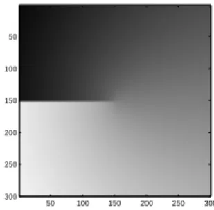
The contours Γi, i = 1, . . . , NC, may be closed contours with ∂Γ = ∅, or open contours with two endpoints. The endpoints may lie on the image boundary ∂Ω, may belong to triple junctions where three curves meet, or may be free endpoints, cf. the conjecture of Mumford and Shah [11]. In the latter case, the endpoint is a point inside the image domain, where no other curve continues. Figure 1 shows an image where an edge occurs which terminates near the image center.

The edge can be represented by a curve with one endpoint located at the left image boundary∂Ωand one endpoint being a free endpoint, located close to the image center.

In [30], we proposed a parametric method for image seg- mentation with piecewise constant image approximations u and interface curvesΓ1, . . . ,ΓN_C, each separating two regions.

There, we considered a decomposition of the image in NR

regions Ω₁, . . . ,Ω_NR separated by curvesΓ_i,i= 1, . . . , N_C,

50 100 150 200 250 300

50

100

150

200

250

300

Fig. 1. Image containing an edge with a free endpoint.

and approximationsu_|Ωk =c_k∈R. In that case, the functional (1) reduces to

E(Γ, c1, . . . , cN_R) =σ|Γ|+λ

N_R

X

k=1

Z

Ωk

(u0−ck)²dx, (2) see [10]. Using methods from the theory of calculus of variations, the following evolution equation can be derived for time-dependent curvesΓ_i(t),t∈[0, T]:

(Vn)i=σκi+Fi, i= 1, . . . , NC, (3) where(Vn)iis the normal velocity ofΓi(t),κiis the curvature, andFi is given by

F_i(. , t) =λ[(u₀−c_k+(i)(t))²−(u₀−c_k−(i)(t))²], (4) with t ∈ [0, T]. The indices k⁺(i), k⁻(i) ∈ {1, . . . , NR} denote the two regions which are separated by Γi(t). The coefficientsck(t),k = 1, . . . , NR, are the mean ofu0 in the regionΩk(t).

In practice, the segmentation problem can be solved in a two-step approach. For discrete time steps t ≥ 0, the coefficientsck are computed using the current set of curves.

This is followed by an update of the curvesΓ(t)→Γ(t+∆t), performed by solving the evolution equation (3).

For some images, the piecewise constant approximation is not applicable, see the exemplary image in Figure 1. For such images, the image domain cannot be decomposed in regions separated by interface curves.

Consequently, we modify the two-step approach of [30], such that also non-interface curves with free endpoints can be dealt with. In the first step, we will solve a diffusion equation in the image domain resulting in a piecewise smooth approxi- mationu. Instead of using the coefficientsck, we will consider for ~p ∈ Γi(t) the limit u^±(~p) = lim_→0,>0u(~p±~νi(~p)), where~νi is a normal vector field onΓi(t). Having computed u, we solve the evolution equation (3) with a modified external term Fi, using u^± instead of constantsc_k^±_(i).

Before, presenting further details, we first consider the regularity of a solution of the Mumford-Shah problem at the free endpoint. Fixing the curvesΓ, letudenote the minimizer of the Mumford-Shah energy (1). At free endpoints, problems concerning the regularity of u occur, cf. [11]. Expressed in polar coordinates (r, φ) centered at the free endpoint, the solutionuis of the form

u(r, φ) =c r^1/2sin(1

2(φ−φ₀)) + ˆv(r, φ), (5)

wherevˆis aC¹-function andc, φ₀are constants, see [33].

For image segmentation, we later need to solve the problem on a discrete set: Let Ω^h be a rectangular grid of nodes covering Ω with grid size h > 0. We replace the second integral on the right hand side of (1) by a sum containing difference quotients of the form

∇ⁱ_hu(~z) = 1

h(u(~z+h~ei)−u(~z)), ~z∈Ω^h, (6) where~ei∈R² are the standard basis vectors ofR²,i= 1,2.

For image segmentation applications, we choose the pixel grid, i.e. we use h = 1. For the approximating sum, we have to exclude terms where the line [~z, ~z+h~e_i] intersects with the curve Γ.

Instead of the original Mumford-Shah functional (1), we thus consider the energy

E^h(Γ, u) =σ|Γ|+ X

~z∈Ω^h s.t.~z+h~e2∈Ω^h

(1−αx(~z))(∇²_hu(~z))²+

+ X

~z∈Ω^h s.t.~z+h~e1∈Ω^h

(1−α_y(~z))(∇¹_hu(~z))²+λ Z

Ω

(u₀−u)²dx,

(7) where α_x(~z), α_y(~z) ∈ [0,1] are scalar terms. If [~z, ~z+h~e₁] intersects with Γ,α_y(~z)is set to1.

A. Example

We consider one single open curve Γ. Let~x: [0,1]→R² with ~x([0,1]) = Γ be a parameterization of the curve. Let

~

x(0)be a free endpoint and let ~x(1) intersect with the image boundary.

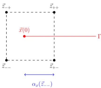
Figure 2 visualizes a possible situation near the free end- point ~x(0). Let ~z₊₊, ~z₊₋, ~z₋₋, ~z₋₊ denote the four grid points around~x(0)as shown in Figure 2. In this example, the tangential vector of the curve at ~x(0) is~τ(0) =~xs(0) =~e1, wheresdenotes the arc-length of the curve.

Considering ~z=~z₊₋, the line[~z₊₋, ~z₊₊]andΓ intersect.

Thus,α_x(~z₊₋)is set to1. For~z=~z₋₋, we define a factor α_x(~z₋₋) := 1

h((~z₊₋)₁−(~x(0))₁), (8) where (.)_i denotes thei-th component of a vector, i= 1,2.

The factor αx(~z₋₋)describes how far the curve has entered the square given by~z++,~z₊₋,~z₋₋,~z₋₊.

For~z∈Ω^h,~z6=~z₋₋, we setα_x(~z) = 0if[~z, ~z+h~e₂]∩Γ =

∅ andα_x(~z) = 1 else. The factor α_y(~z)is defined similarly.

We now want to vary Γ in direction −~τ(0) at ~x(0). We consider a second curve Γ, > 0, with a parameterization

~

x, such that~x(0) =~x(0)−~τ(0). We can assume that is small enough, such that~x(0)is still inside the square given by~z₊₊,~z₊₋,~z₋₋,~z₋₊.

The energy difference is

E^h(Γ, u)−E^h(Γ, u) =σ+ (1−αx(~z₋₋)−)(∇²_hu(~z₋₋))²

−(1−αx(~z−−))(∇²_hu(~z−−))²

=σ−(∇²_hu(~z₋₋))².

Γ

~ z₊₊

~ z+−

~z−−

~z₋₊

~ x(0)

α_x(~z−−)

Fig. 2. Illustration of the pixel grid close to the free endpoint.

The energy will decrease if

σ <(∇²_hu(~z−−))². (9) Thus a motion of a curve in direction −~τ(0) = −~e1 at the free endpoint~x(0) requires that the square of the difference quotient of uin~e2-direction at ~z−− is sufficient large com- pared to the weighting parameter σof the length term in the energy (7).

B. General Case

We consider a curve with one or two free endpoints with tangential vector ~τ(ρ) at the free endpoint ~x(ρ), ρ ∈ {0,1}. We define the factors α_x and α_y as follows: Let

~

z₊₊(ρ), ~z₊₋(ρ), ~z₋₋(ρ), ~z₋₊(ρ) denote the four grid points around~x(ρ).

If ρ= 0and ~τ(0). ~e1 ≥0 or if ρ= 1and~τ(1). ~e1 <0, we define~z^ρ,1:=~z₋₋(ρ)and set

αx(~z^ρ,1) := 1−1

h (~x(ρ))1−(~z^ρ,1)1

.

If ρ= 0and ~τ(0). ~e1 <0 or if ρ= 1and~τ(1). ~e1 ≥0, we define~z^ρ,1:=~z₊₋(ρ)and set

αx(~z^ρ,1) := 1−1

h (~z^ρ,1)1−(~x(ρ))1

.

If ρ= 0and ~τ(0). ~e2 ≥0 or if ρ= 1and~τ(1). ~e2 <0, we define~z^ρ,2:=~z₋₋(ρ)and set

αy(~z^ρ,2) := 1− 1

h (~x(ρ))2−(~z^ρ,2)2

.

If ρ= 0and ~τ(0). ~e2 <0 or if ρ= 1and~τ(1). ~e2 ≥0, we define~z^ρ,2:=~z₋₊(ρ)and set

αy(~z^ρ,2) := 1− 1

h (~z^ρ,2)2−(~x(ρ))2

.

Using these definitions, we define the following factors for

~ z∈Ω^h:

α_x(~z) =











1, if [~z, ~z+h~e₂]∩Γ6=∅, and

~z6=~z^ρ,1, ρ∈ {0,1}, αx(~z^ρ,1), if ~z=~z^ρ,1, ρ∈ {0,1},

0, else.

and

αy(~z) =











1, if [~z, ~z+h~e₁]∩Γ6=∅, and

~

z6=~z^ρ,2, ρ∈ {0,1}, α_y(~z^ρ,2), if ~z=~z^ρ,2, ρ∈ {0,1},

0, else.

For minimizing (7), we propose the following approach:

Assume the case of one curve Γ with two free endpoints parameterized by ~x: [0,1]→R². In the first step, we fix u in (7) and consider for~η : [0,1]→R² a variation of~xof the form ~x+~η, >0.

Let Γ^,η denote the image of ~x+~η. We use the notation E^h(~η) :=E^h(Γ^,η, u)and compute

d d

₌₀

E^h(~η) = d d

₌₀

E^h(Γ^,η, u)

=−σ Z

Γ

~

x_ss. ~ηds− Z

Γ

F ~ν . ~ηds+

+σ~xs(1). ~η(1)−σ~xs(0). ~η(0)

−sign(~τ(1). ~e1)~η(1). ~e1(∇²_hu(~z^1,1))²

−sign(~τ(1). ~e2)~η(1). ~e2(∇¹_hu(~z^1,2))² + sign(~τ(0). ~e₁)~η(0). ~e₁(∇²_hu(~z^0,1))² + sign(~τ(0). ~e₂)~η(0). ~e₂(∇¹_hu(~z^0,2))². For this computation, integration by parts and a transport theorem are applied. Further, ~ν is a normal vector field on Γ such that the pair(~x_s, ~ν)is a positive oriented basis ofR² andF is defined as the jump

F =λ[(u0−u⁺)²−(u0−u⁻)²]. (10) We define the following inner product for functions ~η, ~χ: [0,1]→R²:

(~η, ~χ)_2,Γ,∂Γ:=

Z

Γ

~

η . ~χds+~η(1). ~χ(1) +~η(0). ~χ(0). (11) Now, we consider a family of curves Γ(t),t ∈[0, T]. Let

~

x: [0,1]×[0, T]→ R² be a mapping such that ~x(. , t) is a parameterization of Γ(t),t ∈ [0, T]. We call~x a solution of the gradient flow equation, if

(~xt, ~η)_2,Γ,∂Γ=− d d

₌₀

E^h(~η) (12) holds for all ~η: [0,1]→R².

In the following, we consider particular choices of functions

~

η and derive evolution equations for the curve. First, we consider ~η =η₀~ν for a scalar function η₀ : [0,1]→Rwith η₀(0) =η₀(1) = 0. This provides

Z

Γ(t)

~xt. ~ν η0ds= Z

Γ(t)

(σ~xss. ~ν+F)η0ds.

Since η0 is arbitrary chosen (with value 0 at the endpoints), we conclude the following equation for the normal velocity of the curve:

Vn :=~xt. ~ν =σκ+F, (13a) using the identity

κ~ν=~x_ss. (13b)

Next, we choose~η=η₀~τ, whereη₀: [0,1]→Ris a scalar function withη₀(0)6= 0andη₀(1) = 0, i.e.~η(0) =~τ(0)η₀(0) and~η(1) =~0. Inserting~η in (12), and using (13a), (13b) and

~

τ=~xs, leads to

~

xt(0). ~τ(0)η0(0) =ση0(0)

−sign(~τ(0). ~e₁)~τ(0)η₀(0). ~e₁(∇²_hu(~z^0,1))²+

−sign(~τ(0). ~e₂)~τ(0)η₀(0). ~e₂(∇¹_hu(~z^0,2))².

Since η0(0) is arbitrary and sign(~τ(0). ~ei)~τ(0). ~ei =

|~τ(0). ~ei|for i= 1,2, we conclude for the tangential velocity Vtan(0) :=~xt(0). ~τ(0)

=σ− |~τ(0). ~e1|(∇²_hu(~z^0,1))²

− |~τ(0). ~e2|(∇¹_hu(~z^0,2))². (13c) Choosing η₀(0) = 0 and η₀(1) 6= 0, we can derive the following equation for the tangential velocity in~x(1):

Vtan(1) :=~xt(1). ~τ(1)

=−σ+|~τ(1). ~e1|(∇²_hu(~z^1,1))²

+|~τ(1). ~e₂|(∇¹_hu(~z^1,2))². (13d) Similarly, choosing~η =η0~ν, provides the following equa- tions for the normal velocity at the free endpoints:

V_n(0) :=~x_t(0). ~ν(0)

=−sign(~τ(0). ~e1)~ν(0). ~e1(∇²_hu(~z^0,1))²

−sign(~τ(0). ~e2)~ν(0). ~e2(∇¹_hu(~z^0,2))², (13e) Vn(1) :=~xt(0). ~ν(0)

= + sign(~τ(1). ~e1)~ν(1). ~e1(∇²_hu(~z^1,1))²

+ sign(~τ(1). ~e2)~ν(1). ~e2(∇¹_hu(~z^1,2))². (13f) The curveΓ will grow locally at~x(0), if the curve moves in direction −~τ(0). In this case Vtan(0) =~xt(0). ~τ(0) <0.

Therefore,

σ <|~τ(0). ~e1|(∇²_hu(~z^0,1))²+|~τ(0). ~e2|(∇¹_hu(~z^0,2))|² (14) has to be satisfied such that the curve length increases. For the exemplary case ~τ(0) =~e1, the condition reduces to (9), i.e. to the condition from the introductory example.

The curve Γ(t) will grow at ~x(1), if the curve moves in direction ~τ(1) leading to Vtan(1) > 0. Therefore, the inequality

σ <|~τ(1). ~e₁|(∇²_hu(~z^1,1))²+|~τ(1). ~e₂|(∇¹_hu(~z^1,2))² (15) has to be satisfied.

Since the termσ|Γ|in the energy (7) penalizes the length of the curve, a curve can only grow in direction−~τ(0)or~τ(1), if the derivative terms (∇ⁱ_hu)²,i = 1,2, are large compared toσ.

The scheme (13) describes the motion of the curve. For NC curves Γ1, . . . ,ΓN_C, we can solve (13) for each curve.

For a closed curveΓi, only the normal velocity (13a) with the relation (13b) needs to be considered, on noting that~xi(0) =

~

xi(1). In the case of triple junctions and intersections with the image boundary, additional conditions for the involved

endpoints have to be considered. If triple junctions occur, the evolution equations for the corresponding three curves which meet at the junction are coupled. The cases with triple junctions and boundary intersection points are described in [30] in detail.

We alternately solve the scheme of evolution equations (13) and recompute the approximating function u using the updated curve set. The function u is obtained by solving a diffusion equation on Ω^h. We note that (7) is formulated for a discrete setΩ^h. We will describe in the next section, howu is computed numerically.

III. NUMERICALAPPROXIMATION

A. Numerical Solution of the Evolution Equations

For computing the position of the evolving curvesΓnumer- ically, we consider a decomposition of the interval[0,1]of the form 0 =q₀ⁱ < qⁱ₁ < . . . < q_Nⁱ_i = 1, for i = 1, . . . , NC. If Γi is a closed curve, we make use of the periodicityNi= 0, N_i+ 1 = 1,−1 =N_i−1, etc.

Further, let0 =t0< t1< . . . < tM =T be a partitioning of the time interval[0, T]with time steps∆tm:=tm+1−tm, m = 0, . . . , M−1. Smooth curves Γi(tm), i = 1, . . . , NC, m= 0, . . . , M are replaced by polygonal curvesΓ^m_i given by nodesX~_i,j^m which are approximations of~xi(qⁱ_j, tm). Further, let κ^m_i,j be an approximation of κi(qⁱ_j, tm). The derivative terms with respect to time are replaced by difference quotients of the form

(~x_i)_t(q^j_i, t_m)≈ 1

∆tm

X~_i,j^m+1−X~_i,j^m

. (16)

Leth^m_i,j−1 2

=X~_i,j^m−X~_i,j−1^m ,i= 1, . . . , NC,j= 1, . . . , Ni, be the distance between two neighboring nodes. For each curve, we define a discete normal vector field ~ν_i^mby

~ ν_i^m|_[qi

j−1,q_jⁱ]:=~ν^m_i,j−1 2

:=(X~_i,j^m−X~_i,j−1^m )^⊥ h^m

i,j−¹₂

,

see also [30], [34], [35]. Here, ⊥denotes the anti-clockwise rotation of a vector by π/2. Further, we define the following weighted approximating normal vector at X~_i,j^m by

~ ω^m_i,j:=

h^m_i,j−1 2

~ ν_i,j−^m 1

2

+h^m_i,j+1 2

~ν_i,j+^m 1 2

h^m

i,j−¹₂ +h^m

i,j+¹₂

=(X~_i,j+1^m −X~_i,j−1^m )^⊥ h^m

i,j−¹₂ +h^m

i,j+¹₂

,

for j = 1, . . . , Ni if ∂Γ^m_i =∅ and for j = 1, . . . , Ni−1 if

∂Γ^m_i 6=∅. In the latter case, we set

~

ω^m_i,0:=~ν^m_i,1 2

=(X~_i,1^m−X~_i,0^m)^⊥ h^m

i,¹₂

,

~

ω_i,N^m _i:=~ν^m_i,N

i−¹₂ = (X~_i,N^m

i−X~_i,N^m

i−1)^⊥ h^m_i,N

i−¹₂

.

The external term F is approximated by F_i,j^m:=λh

(u₀(X~_i,j^m)−u(X~_i,j^m +a~ω^m_i,j))²

−(u0(X~_i,j^m)−u(X~_i,j^m−a~ω_i,j^m))²i ,

with a small real numbera >0ifj is not the index of a free endpoint, and we set F_i,j^m= 0 else.

The equation for the normal velocity (13a) is approximated by

1

∆tm

X~_i,j^m+1−X~_i,j^m

. ~ω^m_i,j=σκ^m+1_i,j +F_i,j^m. (17a) Thus, for computingΓ^m+1_i , we use the previous curveΓ^m_i for the external termF_i,j^m and for the weighted normal ~ω_i,j^m.

For an approximation of (13b), we need to define an approximation of (~xi)ss(q_jⁱ, tm+1). For that, we make use of difference quotients of the form

∆^h,m₂ X~_i,j^m+1:= 2 h^m_i,j−1

2

+h^m_i,j+1 2

(X~_i,j+1^m+1 −X~_i,j^m+1)/h^m_i,j+1 2

−(X~_i,j^m+1−X~_i,j−1^m+1)/h^m_i,j−1 2

,

for i = 1, . . . , NC and j = 1, . . . , Ni, if ∂Γ^m_i = ∅, and j = 1, . . . , Ni−1, else. In case of equal spatial step sizes h^m_i,j−1

2

=h^m_i,j+1 2

=:h^m_i , the term reduces to(X~_i,j−1^m −2X~_i,j^m+ X~_i,j+1^m )/((h^m_i )²), see also [30], where we also defined and used these difference quotients.

The equation (13b) is now approximated by

κ^m+1_i,j ~ω_i,j^m = ∆^h,m₂ X~_i,j^m+1, (17b) fori= 1, . . . , NC,j= 1, . . . , Ni in case of closed curves and j= 1, . . . , Ni−1 in case of open curves.

In case of open curves, additional equations for the end- points are needed. The case of triple junctions and boundary intersection points is described in [30]. For curves with free endpoints we introduce the tangential vectors ~τ_i,0^m = (X~_i,1^m − X~_i,0^m)/h_i,1

2, and ~τ_i,N^m

i = (X~_i,N^m

i −X~_i,N^m

i−1)/h_i,Ni−1 2. The equations (13c) and (13d) are approximated by

1

∆tm

X~_i,0^m+1−X~_i,0^m . ~τ_i,0^m =

=σ− |~τ_i,0^m. ~e₁|(∇²_hu(~z^0,1))²− |~τ_i,0^m. ~e₂|(∇¹_hu(~z^0,2))², (17c) and

1

∆tm

X~_i,N^m+1

i −X~_i,N^m_i

. ~τ_i,N^m_i =

=−σ+|~τ_i,N^m

i. ~e₁|(∇²_hu(~z^1,1))²+|~τ_i,N^m

i. ~e₂|(∇¹_hu(~z^1,2))². (17d) Similarly, discrete versions of (13e) and (13f) can be stated using ~ω^m_i,0 and~ω^m_i,N

i as discrete normal vectors.

The scheme (17) is a numerical approximation of the scheme (13), where the parametric curves are replaced by polygonal curves, and the smooth functions ~xi and κi are replaced by continuous functions uniquely given by their values at the nodes q_jⁱ,i= 1, . . . , NC,j= 0, . . . , Ni.

The discrete scheme can be rewritten to a linear system with a sparse system matrix, similar as presented in [30], and can be solved with a fast direct solver like for example the UMFPACK algorithm [36].

B. Numerical Solution of the Denoising Problem

For computing a numerical solution u^h for the piecewise smooth, denoised versionuofu₀, we consider forN_x, N_y∈N the discrete set

Ω^h:={(ih, jh) : i= 0, . . . , Nx, j= 0. . . , Ny}, where N_x and N_y are the number of pixels in x- and y- direction. We define for i= 1, . . . , N_x,j= 1, . . . , N_y

Ax(i, j) =







h², if [(i−1)h, ih]× {j} ∩Γ^m_i0 =∅,

∀i0∈ {1, . . . , NC}, 0, else,

Ay(i, j) =







h², if {i} ×[(j−1)h, jh]∩Γ^m_i0 =∅,

∀i0∈ {1, . . . , NC}, 0, else.

Fixing the set of curves Γ, we consider the following discrete energy:

Ediscr(u^h) =

N_x

X

i=1 Ny

X

j=1



Ax(i, j) u^h_i,j−u^h_i−1,j h

!2

+A_y(i, j) u^h_i,j−u^h_i,j−1 h

!²



+λ

N_x

X

i=0 Ny

X

j=0

h² u0(ih, jh)−u^h_i,j²

, (18)

which is a discrete analogue of

R

Ω\Γ k∇uk²dx+R

Ωλ(u0−u)²

dx. Here u^h_i,j approximates u at the node (ih, jh). The piecewise continuous function u^h is uniquely given by its value at the points in Ω^h.

By setting the terms Ax(i, j) or Ay(i, j) to zero at points where the line [(i −1)h, jh),(ih, jh)] or [(ih,(j − 1)h),(ih, jh)]intersects with one of the curves, we approxi- mate the integral over the set Ω\Γ.

Taking the derivative of the right hand side of (18) with respect to u^h_i,j and setting the resulting term to zero, leads to a linear system. The corresponding system matrix is sparse since each node (ih, jh) ∈ Ω^h is only coupled to a few neighboring nodes. The resulting linear system can be solved with a fast direct or iterative solver by employing the sparse matrix structure.

Considering h→ 0, we obtain in the limit ∇u . ~ν = 0 at the curves belonging to Γ, and ∇u . ~n_∂Ω = 0 at the image boundary ∂Ω, where~n_∂Ω is a normal vector field at∂Ω. For details, we refer to [30]. Consequently, we obtain an edge preserving image smoothing if Γ matches with the edges in the given image.

C. Topology Changes

During the evolution of curves, topology changes can occur, since the edge set in the image and the boundaries of objects are not known in advance. Therefore, curves can split into

two or more subcurves, curves can merge to one single curve, triple junctions and new curves may occur and curves can intersect with the image boundary such that new boundary nodes emerge. Further, a curve needs to be deleted if its length becomes too small. In [30], we extended the idea of [31], [32], and described a method to detect topology changes of curves efficiently. The main idea is the use of an artificial background grid which covers the entire image domain Ω. We consider successively all nodesX~_i,j^m and mark a grid element with(i, j) ifX~_i,j^m is the first node located in this array. If a grid element is already marked with(i1, j1)and the nodesX~_i,j^m andX~_i^m_1,j1 are not neighbor nodes, a topology change likely occurs close to this pair. Details on this method for curves without free endpoints are given in [30].

In principle, topology changes involving curves with free endpoints can be detected similarly by using such a back- ground grid. In addition to the topology changes listed above (splitting, merging, emergence of triple junctions and bound- ary intersection points), topology changes involving the free endpoints can occur: If two free endpoints of one curve are located in one square of the background grid, an open contour becomes a closed contour. If two free endpoints of two different curves meet, the two curves merge to one single curve, and the former free endpoints become inner nodes of the new curve. If a free endpoint and an inner point of a curve meet, a triple junction is created.

D. Summary of the Algorithm

We propose the following algorithm for image segmentation and image restoration with parametric contours with possible free endpoints:

Given a set of polygonal curves Γ⁰ = (Γ⁰₁, . . . ,Γ⁰_N

C) and X~⁰ = (X~₁⁰, . . . , ~X_N⁰

C) with X~_i⁰([0,1]) = Γ⁰_i, perform the following steps form= 0,1, . . . , M−1:

1) Compute a denoised image approximationu^h by mini- mizing (18) (solve the corresponding sparse linear sys- tem).

2) Compute the external termsF_i,j^mby using the solutionu^h of step 1. ComputeX~^m+1by solving the linear equation derived from the scheme (17).

3) Check whether topology changes occur. If so, execute the topology change.

A segmentation of the image is given by the final set of curves Γ^M. An image restoration is given by the image approximation u^hfrom the time steptM.

E. Modifications

Step 2 of the algorithm above can additionally be split in two sub-steps: First, we fix the free endpoints and we let the inner nodes of the curve evolve. Then, we let the endpoints evolve according to the above presented discrete scheme.

The main effort of this method compared to the Chan-Vese method for interface curves is that we have to solve a two- dimensional diffusion equation (bulk equation) several times during the segmentation. In the experiments described in the next section, we perform 10 steps of curve evolution followed

by a solution of the bulk equation. Having computed u^h, we use it for the next 10 curve evolution steps.

As an alternative, we can start the segmentation using interface curves and the image segmentation method described in [30] (based on the Chan-Vese method [10]) with piecewise constant approximations. As a postprocessing step, we can consider the derivatives of the image function in normal direction at the final curves (or the jump of the image function across the curves). We replace interface curves by curves with free endpoints if the derivatives in normal direction are locally very small. For that, we delete those parts of a curve where the derivative is small which results in curves with free endpoints.

Next, we compute some steps of the segmentation method with free endpoints to obtain the final contours.

Topology changes occur only in rare cases when using a postprocessing evolution of curves with free endpoints. In most situations, topology changes are already detected in the previous evolution.

IV. RESULTS ANDDISCUSSION

The method for image segmentation and restoration pre- sented in sections II and III are applied on some exemplary test images. For all experiments presented in this section, we use constant time steps sizes ∆t_m= ∆t,m= 0, . . . , M−1.

In the first experiment, we consider an example where a contour with two free endpoints evolves in the image domain and detects an edge. Figure 3 presents the results of image segmentation and denoising. It can be observed that the image is not smoothed out across the curve Γ. Further a growth of the curve in tangential direction can be observed. The growth stops when the inequalities (14) and (15) become equalities.

This depends on the absolute values of the difference quotients

|∇ⁱ_hu|,i = 1,2, and the weighting parameter σ. The image approximationuattends values in[0,1]. In this image, differ- ences of the formu(~x+h~e_i)−u(~x)are typically of magnitude 10⁻². Since Ω = [1,300]×[1,300]andh= 1, |∇ⁱ_hu|² is of magnitude 10⁻⁴. Therefore, we have to choose a small value for the weighting parameter σ, here, we choose σ= 2e−5.

If we used a normalized image domain Ω = [0,1]×[0,1], the pixel grid would have a grid size of h = 1/300 and h² = 1/90000. In this case, we would choose a weight σ of magnitude1.

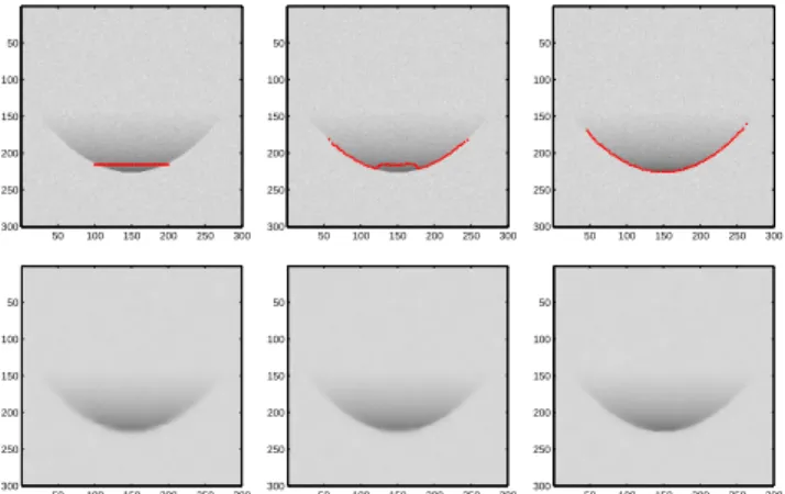
In a second experiment, we study a crack tip problem which has also been considered in [28]. The image function is given by

u0(~x) =ap

r(~x) sin(θ(~x)/2) +b, (19) where r(~x) ≥0, θ(~x) ∈ (−π, π] are polar coordinates with r = 0 corresponding to the image center, and a, b ∈ R are constants such that u0 attends values in [0,1].

Figure 4 shows the evolution of a contour with one free endpoint. The second endpoint belongs to the image boundary.

At time step m = 3000, the free endpoint is located at the image center and the curve matches with the edge in the image. As discussed above (see also Equations (14) and (15)), the parameter σ, which weights the length term, needs to be chosen small enough such that the curve can extend. If σ is fixed, the absolute value of the difference quotients must be

50 100 150 200 250 300 50

100

150

200

250

300

50 100 150 200 250 300

50

100

150

200

250

300

50 100 150 200 250 300

50

100

150

200

250

300

50 100 150 200 250 300 50

100

150

200

250

300

50 100 150 200 250 300

50

100

150

200

250

300

50 100 150 200 250 300

50

100

150

200

250

300

Fig. 3. Example image showing a contour with two free endpoints. Original image and evolving contours (1st row) and denoised image (2nd row) for m= 1,1000,6000using∆t= 0.032,σ= 2e−5andλ= 0.002.

50 100 150 200 250 300 50

100

150

200

250

300

50 100 150 200 250 300

50

100

150

200

250

300

50 100 150 200 250 300

50

100

150

200

250

300

Fig. 4. Example image showing a contour with one free endpoint and one boundary intersection point, see also [28]. Evolving contours form= 1,500,3000using∆t= 0.001,σ= 2e−5andλ= 0.002.

large enough such that the length of the curve increases. In this example, the edge is a horizontal line and the position where the curve stops depends on the value of ∇²_hu, i.e. on the difference quotient iny-direction.

We rerun the example using σ = 0.002 and σ = 0.01 instead of σ = 2e−5. Figure 5 shows the results at time step m = 3000. In both cases, the free endpoint does not reach the center of the image since the value of σ has been set larger. The growth of the curve already stops at larger values of∇²_hu, recall conditions (14) and (15)). We even let the curve evolve until time step m= 5000, but we observed no significant motion betweenm= 3000andm= 5000.

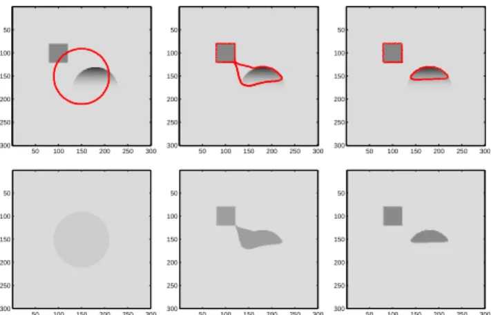
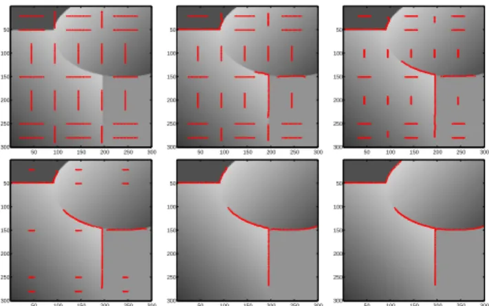
In another experiment, which demonstrates the evolution of curves with free endpoints, we first apply the parametric method of [30] to the Chan-Vese problem [10] using interface- curves. This means, that we first segment a given image in regions separated by interface curves, see Figure 6. We start with one large initial curve which splits up in two sub- curves. This example thus also demonstrates the handling of a topology change.

In a postprocessing step, we delete those nodes where the jump ofu0across the curve is smaller than a given tolerance of tol = 0.1. This results in one closed curve, where no points are deleted (blue curve in Figure 7), and in one curve with two free endpoints (red curve). Figure 7 shows the results of a postprocessing evolution of the curve. This example shows that our methods for image segmentation and denoising can be applied also on images with both open and closed edges.

Table I shows the values of the discrete Mumford-Shah

50 100 150 200 250 300 50

100

150

200

250

300

50 100 150 200 250 300

50

100

150

200

250

300

Fig. 5. Dependency on the weighting parameter usingσ= 0.002(left) and σ = 0.01(right),∆t= 0.001andλ = 0.002for m = 3000. If a too large weight is chosen for the length term in (7), the curve does not reach the image center.

50 100 150 200 250 300 50

100

150

200

250

300

50 100 150 200 250 300 50

100

150

200

250

300

50 100 150 200 250 300 50

100

150

200

250

300

50 100 150 200 250 300 50

100

150

200

250

300

50 100 150 200 250 300 50

100

150

200

250

300

50 100 150 200 250 300 50

100

150

200

250

300

Fig. 6. Image segmentation result using Chan-Vese, interface curves and a piecewise constant image approximation. Original image and contours (first row) and piecewise constant approximation (second row) for m = 1,1050,1200.

TABLE I

COMPARISON OF DISCRETEMUMFORD-SHAHENERGY Processing Method Step Nr Discrete

Mumford-Shah Energy Chan-Vese,

piecewise constant

1200 (final) 22364.94 Postprocessing, free

endpoints

1 (start) 23162.04 Postprocessing, free

endpoints

400 (final) 18284.36

energy (7) for the last step of the Chan-Vese piecewise constant segmentation with closed region boundaries (cf. Figure 6, m = 1200) and for the initial and final step of the postpro- cessing with one open boundary (cp. Figure 7, m = 1 and m= 400). Note, that the absolute values are large, since the image consists of 90000 pixels and the size of each pixel is 1×1. The average contribution of each pixel to the energy is

<1; however, it sums up to a value of magnitude2·10⁴. From Table I, we can observe that the energy even slightly increases from the last step of the Chan-Vese piecewise con- stant method to the first step of the postprocessing evolution.

Deleting part of the curve doesnotdecrease the energy in this example. However, at the end of the postprocessing evolution with one open contour, we obtain a decrease of the energy.

The energy atm= 400of the postprocessing is81.75%of the

50 100 150 200 250 300 50

100

150

200

250

300

50 100 150 200 250 300

50

100

150

200

250

300

50 100 150 200 250 300

50

100

150

200

250

300

Fig. 7. Postprocessing evolution with a contour with two free endpoints usingtol= 0.1 to obtain the initial contour. Original image and contours (left, center) form= 1,400using∆t= 0.05,σ= 2e−5,λ= 2e−4and denoised image form= 400(right).

50 100 150 200 250 300 50

100

150

200

250

300

50 100 150 200 250 300

50

100

150

200

250

300

50 100 150 200 250 300

50

100

150

200

250

300

Fig. 8. Postprocessing evolution with a contour with two free endpoints usingtol= 0.5 to obtain the initial contour. Original image and contours (left, center) form= 1,600using∆t= 0.05,σ= 2e−5,λ= 2e−4and denoised image form= 600(right).

energy of the last step of the piecewise constant segmentation with closed boundaries. Therefore, if we delete part of the curve and if we let the curve with free endpoints evolve again, we will obtain a final curve such that the corresponding discrete Mumford-Shah energy (7) is reduced compared to the Chan-Vese piecewise constant result.

Next, we investigate the influence of the tolerance valuetol, which is used for the deletion of some nodes of the curve.

Note, that the image function attends values in[0,1]where0 corresponds to black and 1 corresponds to white color. The exact value of the tolerancetolinfluences only the start curve of the second curve evolution. We repeat the postprocessing evolution and usetol= 0.5as tolerance resulting in a different initial curve.

Figure 8 shows the postprocessing evolution of the curve.

Of course, since the initial contour in Figure 8 (left) is smaller compared to the initial contour in Figure 7, more iteration steps are needed to obtain the final contour.

The final result is independent on the exact initial curve as long as it is of the same type, i.e. open with free endpoints;

not closed or not fully deleted. In our example the largest jump of u₀ across the final red curve of the first evolution (cf. Figure 6, right sub-figures) is 0.61, the smallest jump is 0.05. The large difference between the largest and smallest jump can be used as an indicator to replace the interface- curve by a curve with two free endpoints. (On the contrary, the jump across the blue curve is constant in this example.) As tolerance valuetolany value larger than0.05and smaller than 0.61 could be chosen. For tol ≤ 0.05 no node point would be deleted resulting in an unchanged curve. For tol ≥ 0.61 all nodes and therefore the entire curve would be deleted. All values between the two thresholds can be theoretically used.

Therefore, in this example, the final result is independent on the exact value oftol as long it is in(0.05,0.61).