Uncertainty-based image segmentation with unsupervised mixture models

Uncertainty-Based Image

Segmentation with Unsupervised Mixture Models

Von der Fakultät für

Elektrotechnik und Informationstechnik der Technischen Universität Dortmund

genehmigte

Dissertation

zur Erlangung des akademischen Grades Doktor der Ingenieurwissenschaften (Dr.-Ing.)

von

Thorsten Wilhelm Dortmund, 2019

Tag der mündlichen Prüfung: 30.10.2019

Hauptreferent: Prof. Dr. rer. nat. Christian Wöhler Korreferent: Prof. Dr.-Ing Franz Kummert

Arbeitsgebiet Bildsignalverarbeitung Technische Universität Dortmund

A C K N O W L E D G E M E N T S

First of all, I would like thank my supervisor Prof. Dr. rer. net. Christian Wöhler for giving me the opportunity to pursue a PhD. Thank you for giving me the freedom to work on my own ideas and sharing your knowledge with me. Further, I would like to thank Prof. Dr.-Ing. Franz Kummert for agreeing to be my second reviewer.

I would like to thank Prof. Dr.-Ing. Gernot A. Fink and Dr.-Ing. Rene Grzeszick for providing a wonderful working atmosphere in the DFG-project

we have been working on sucessfully. In great parts this project enabled the creation of this thesis.

In the last four years of being a research assistant at TU Dortmund University, I was fortunate enough to work in a pleasant working atmosphere with skilful colleagues.

Special thanks to Malte Lenoch and Kay Wohlfarth for doing all the administrative stuff at the Image Analysis Group. Thanks to all the current and former members of the group I was happy to work with. I’m also thankful to my colleagues from the Information Processing Lab for the many fun hours we shared at table football. I would also like to thank the staff of the Pattern Recognition in Embedded Systems Group for the occasional drinks we shared and the fruitful discussions at work and afterwards. I wish you all the best for your own projects.

I’m in-depth grateful to Marcel Hess, Dominik Koßmann, Leonard Rothacker, and Kay Wohlfarth for taking their precious time to read through earlier versions of this manuscript and the valuable feedback they provided. Thank you.

I want to thank my friends and family for providing the right distractions at the right times and I’m grateful to my parents who have always supported me unconditionally.

Lastly, I want to thank my wonderful wife. Jenny, I thank you whole-heartedly for your patience and support, giving me the freedom to pursue my dreams. And thank you, Leah, for providing just the right motivation to actually finish this thesis. I’m looking forward to seeing you.

Dortmund, April 21, 2019

1 Project number269661170

iii

A B S T R A C T

In this thesis, a contribution to explainable artificial intelligence is made. More specifi- cally, the aspect of artificial intelligence which focusses on recreating the human percep- tion is tackled from a previously neglected direction. A variant of human perception is building a mental model of the extents of semantic objects which appear in the field of view. If this task is performed by an algorithm, it is termed image segmentation. Recent methods in this area are mostly trained in a supervised fashion by exploiting an as exten- sive as possible data set of ground truth segmentations. Further, semantic segmentation is almost exclusively tackled by Deep Neural Networks (DNNs).

Both trends pose several issues. First, the annotations have to be acquired somehow.

This is especially inconvenient if, for instance, a new sensor becomes available, new do- mains are explored, or different quantities become of interest. In each case, the cumber- some and potentially costly labelling of the raw data has to be redone. While annotating keywords to an image can be achieved in a reasonable amount of time, annotating ev- ery pixel of an image with its respective ground truth class is an order of magnitudes more time-consuming. Unfortunately, the quality of the labels is an issue as well be- cause fine-grained structures like hair, grass, or the boundaries of biological cells have to be outlined exactly in image segmentation in order to derive meaningful conclusions.

Second, DNNs are discriminative models. They simply learn to separate the features of the respective classes. While this works exceptionally well if enough data is provided, quantifying the uncertainty with which a prediction is made is then not directly possi- ble. In order to allow this, the models have to be designed differently. This is achieved through generatively modelling the distribution of the features instead of learning the boundaries between classes. Hence, image segmentation is tackled from a generative perspective in this thesis. By utilizing mixture models which belong to the set of gen- erative models, the quantification of uncertainty is an implicit property. Additionally, the dire need of annotations can be reduced because mixture models are conveniently estimated in the unsupervised setting.

Starting with the computation of the upper bounds of commonly used probability distributions, this knowledge is used to build a novel probability distribution. It is based on flexible marginal distributions and a copula which models the dependence structure of multiple features. This modular approach allows great flexibility and shows excellent performance at image segmentation. After deriving the upper bounds, different ways to reach them in an unsupervised fashion are presented. Including the probable locations of edges in the unsupervised model estimation greatly increases the performance. The proposed models surpass state-of-the-art accuracies in the generative and unsupervised setting and are on-par with many discriminative models. The analyses are conducted following the Bayesian paradigm which allows computing uncertainty estimates of the model parameters. Finally, a novel approach combining a discriminative DNN and a local appearance model in a weakly supervised setting is presented. This combination yields a generative semantic segmentation model with minimal annotation effort.

v

K U R Z FA S S U N G

In dieser Arbeit wird ein Beitrag zur Interpretierbarkeit von künstlichen Intelligenzen vorgestellt. Der Teilaspekt der künstlichen Intelligenz, der sich der Nachbildung der menschlichen Wahrnehmung widmet, wird von einer bisher vernachlässigten Richtung aus neu betrachtet. Die menschliche Wahrnehmung erstellt ein mentales Modell der Größe von semantischen Objekten, die ein Mensch sieht. Wird diese Aufgabe von einer Maschine durchgeführt spricht man von einer Bildsegmentierung. Aktuelle Ansätze in diesem Bereich nutzen nahezu ausschließlich tiefe neuronale Netze, die mit riesigen Mengen an annotierten Daten überwacht trainiert werden.

Dies hat jedoch zur Folge, dass sobald neue Sensoren, neue Domänen oder schlicht andere Größen von Interesse sind, das mühsame Annotieren der Daten erneut durchge- führt werden muss. Eine Annotation durch Schlüsselwörter kann unter Umständen in einem zeitlich vertretbaren Rahmen durchgeführt werden. Allerdings werden zum Trainieren von Segmentierungsnetzen Annotationen für jedes Pixel eines Bildes benötigt.

Außerdem ist die Qualität der Annotation im Auge zu behalten, da nur so feine Struk- turen wie Haare, Gras oder die genauen Grenzen biologischer Zellen erhalten bleiben.

Weiterhin sind tiefe neuronal Netze diskriminative Klassifikatoren und lernen die Daten der unterschiedlichen Klassen zu trennen. In der Praxis funktioniert dieser Ansatz sehr gut, wenn genug Trainingsmaterial vorhanden ist. Allerdings ist in diesem Szenario keine Angabe von Unsicherheiten bei der Klassifikation möglich. Um dies zu erreichen muss die Verteilung der Daten aller Klassen geschätzt werden. Eine Methode, die das ermöglicht sind Mischverteilungsmodelle, die generativ die Verteilung der Daten im Raum mit Wahrscheinlichkeitsverteilungen nachbilden. Zusätzlich kann in diesem Fall auf Annotation verzichtet werden.

In dieser Arbeit werden zunächst die oberen Schranken der Genauigkeiten beim Segmentieren von Bildern mit verschiedenen Wahrscheinlichkeitsverteilungen berech- net. Dieses Wissen wird anschließend genutzt um eine Wahrscheinlichkeitsverteilung einzuführen, die auf flexiblen Randverteilungen und einer Copula basiert, die die Ab- hängigkeiten von mehreren Merkmalen modelliert. Dieser modulare Ansatz ermöglicht es sehr flexibel Verteilungen zu kreieren und zeigt eine sehr hohe Genauigkeit beim Seg- mentieren von Bilddaten. Im Anschluss werden Ansätze präsentiert wie die überwacht gelernte obere Schrank im unüberwachten Fall erreicht werden kann. Hier hat sich vor allem das probabilistische Modellieren für das Auftreten von Kanten als äußerst wichtig herausgestellt. Die vorgestellten Modelle übertreffen den aktuellen Stand der Technik vergleichbarer Modelle und werden im Sinne der Bayes-Statistik geschätzt. Dieses Vorge- hen ermöglicht die Angabe von Unsicherheiten in der Schätzung der Modellparame- ter. Abschließend wird in dieser Arbeit eine Methode vorgestellt, die es ermöglicht ein diskriminativ trainiertes tiefes neuronales Netz mit einem lokalen Model zur Beschrei- bung der visuellen Erscheinung zu kombinieren. Das tiefe Netz wird dabei nur mit schwacher Überwachung trainiert. Die Kombination beider Ansätze ermöglicht es Bilder mit minimalem Annotationsaufwand semantisch zu segmentieren und außerdem Un- sicherheiten in der Segmentierung anzugeben.

vii

P U B L I C AT I O N S

This thesis is based on the following publications of the author. The publications are listed in ascending chronological order.

Peer-reviewed conference contributions

[WW16] T. Wilhelm and C. Wöhler. “Flexible Mixture Models for Colour Image Seg- mentation of Natural Images.” In:

International Conference on Digital Image Computing: Techniques and Applications (DICTA). 2016, pp. 1–7.

[WW17c] T. Wilhelm and C. Wöhler. “Improving Bayesian Mixture Models for Colour Image Segmentation with Superpixels.” In: Proceedings of the

Conference on Computer Vision, Imaging and Computer Graphics Theory and Applications - Volume

2017, pp. 443–450.

[WW17a] T. Wilhelm and C. Wöhler. “Boundary aware image segmentation with unsu- pervised mixture models.” In:

IEEE International Conference on Image Processing (ICIP). 2017, pp. 3325–3329.

[Wil +17] T. Wilhelm, R. Grzeszick, G. A. Fink, and C. Wöhler. “From Weakly Super- vised Object Localization to Semantic Segmentation by Probabilistic Image Mod- eling.” In:

International Conference on Digital Image Computing: Techniques and Applications (DICTA). 2017, pp. 1–7.

[WW17b] T. Wilhelm and C. Wöhler. “On the suitability of different probability dis- tributions for the task of image segmentation.” In:

International Conference on Image and Vision Computing New Zealand (IVCNZ). 2017, pp. 1–6.

Other publications which are not part of this thesis and co-authored work is listed in ascending chronological order in the following.

Peer-reviewed conference contributions

[LWW16] M. Lenoch, T. Wilhelm, and C. Wöhler. “Simultaneous Surface Segmentation and BRDF Estimation via Bayesian Methods.” In: Proceedings of the

ference on Computer Vision, Imaging and Computer Graphics Theory and Applications - Volume

2016, pp. 39–48.

[Woh+ 18] K. Wohlfarth, C. Schröer, M. Klaß, S. Hakenes, M. Venhaus, S. Kauffmann, T. Wilhelm, and C. Wöhler. “Dense Cloud Classification on Multispectral Satellite Imagery.” In:

(PRRS). 2018, pp. 1–6.

[Wil +19] T. Wilhelm, R. Grzeszick, G. Fink, and C. Wöhler. “Unsupervised Learning of Scene Categories on the Lunar Surface.” In: Proceedings of the

ix

Invited Talks

Thorsten Wilhelm. “Restraining AI’s hunger for annotated training data—weak super- vision in autonomous driving.” Image Sensors Auto Europe

2019

x

C O N T E N T S

1 introduction 1

1.1 Contribution . . . . 2

1.2 Outline . . . . 2

2 image segmentation 5 2.1 Fundamentals of Probability Theory . . . . 6

2.2 The Data . . . . 8

2.3 Levels of Supervision . . . . 10

2.3.1 Unsupervised Learning . . . . 11

2.3.2 Supervised Learning . . . . 12

2.3.3 Semi-Supervised Learning . . . . 13

2.3.4 Weakly-Supervised Learning . . . . 13

2.4 Model-based Approaches . . . . 14

2.4.1 Thresholding . . . . 14

2.4.2 K-Means Clustering . . . . 14

2.4.3 Gaussian Mixture Models . . . . 16

2.4.4 Mixture of t-Distributions . . . . 17

2.5 Distance-based Approaches . . . . 18

2.5.1 Mean-shift . . . . 18

2.5.2 Normalized Cuts . . . . 19

2.6 Contour Detection . . . . 20

2.6.1 Feature Computation and Cue Combination . . . . 20

2.6.2 Enforcing Closed Contours . . . . 21

2.7 Superpixels . . . . 22

2.8 Semantic Segmentation . . . . 23

2.8.1 History of Deep Neural Networks . . . . 23

2.8.2 Deep Neural Networks in Semantic Segmentation . . . . 24

2.8.3 Class Activation Maps . . . . 25

2.9 Scene and Object Detection Tasks . . . . 25

2.10 Image Segmentation Tasks . . . . 26

2.10.1 BSDS300 and BSDS500 . . . . 27

2.10.2 VOC2012 . . . . 28

2.10.3 LeafSnap Field Data Set . . . . 28

2.10.4 Others . . . . 28

2.11 Measuring the Performance of Image Segmentation . . . . 28

2.11.1 Object-based Measures . . . . 29

2.11.2 Partition-based Measures . . . . 30

2.11.3 Boundary-based Measures . . . . 32

2.11.4 Summary . . . . 32

3 fundamentals of bayesian inference 33 3.1 The Prior - Subjectivism in Data Analysis . . . . 33

3.2 Probability Distributions . . . . 34

3.2.1 Discrete Probability Distributions . . . . 34

xi

3.2.2 Continuous Distributions . . . . 35

3.2.3 Multivariate Distributions . . . . 41

3.2.4 Mixture Models . . . . 44

3.3 Model Comparison . . . . 46

3.3.1 Statistical Approaches . . . . 47

3.3.2 Cluster Validation Criteria . . . . 48

3.4 Markov Chain Monte Carlo . . . . 49

3.4.1 Monte Carlo Integration and Markov Chains . . . . 50

3.4.2 Metropolis-Hastings . . . . 51

3.4.3 Delayed Rejection Adaptive Sampling . . . . 53

3.4.4 Others . . . . 53

3.5 Non-parametric Approaches . . . . 54

3.5.1 Infinite Mixture Models . . . . 54

3.5.2 Kernel Density Estimation . . . . 55

3.6 Copula . . . . 56

3.6.1 Gaussian Copula . . . . 58

3.7 Significance Testing . . . . 59

4 suitability of various probability distributions inside a mix- ture model 61 4.1 Model Assumptions . . . . 61

4.2 Colour Spaces . . . . 63

4.3 Positional Data . . . . 65

4.4 Univariate vs. Multivariate Distributions . . . . 68

4.5 Distributions . . . . 69

4.5.1 Sinh-asinh Copula . . . . 70

4.6 Accuracy Assessment . . . . 71

4.7 Summary . . . . 73

4.8 Future Research Directions . . . . 74

5 superpixel based image segmenation 77 5.1 Superpixels in Generative Modelling . . . . 77

5.1.1 Subsampling vs. Superpxixels . . . . 78

5.1.2 Building a Texture Feature from Superpixels . . . . 80

5.2 Determining an Appropriate Number of Mixture Components . . . . 81

5.2.1 Cluster Validation Criteria . . . . 81

5.2.2 Regression Based Approaches . . . . 82

5.2.3 Infinite Mixture Models . . . . 84

5.2.4 Results . . . . 85

5.3 Model Definition and Parameter Estimation . . . . 86

5.3.1 Accuracy Assessment . . . . 90

5.4 Including Edges as a Boundary Prior . . . . 92

5.4.1 Passive Edge Model . . . . 93

5.4.2 Active Edge Movement . . . . 95

5.4.3 Accuracy Assessment . . . . 96

5.5 Comparison to Other Approaches . . . . 97

5.6 Summary . . . . 100

5.7 Future Research Directions . . . . 101

contents xiii

6 weakly supervised object localization and semantic segmenta-

tion 103

6.1 Related Work . . . . 103

6.2 Recent Developments . . . . 106

6.3 Fusing Class Activation Maps with Density Estimation . . . . 106

6.3.1 Class Activation Maps . . . . 107

6.3.2 Segmentation . . . . 108

6.3.3 Combining Class Activation Maps with KDE . . . . 109

6.3.4 Localization . . . . 109

6.4 Evaluation . . . . 110

6.4.1 Qualitative Results . . . . 111

6.4.2 Segmentation Accuracy . . . . 111

6.4.3 CorLoc Metric . . . . 113

6.5 Summary . . . . 114

7 conclusion 115

bibliography 117

Figure 2.1 Gradient Image . . . . 9

Figure 2.2 Filterbank . . . . 10

Figure 2.3 Visualisation of different annotations of one image in the BSDS500 11 Figure 2.4 VOC Detection Task . . . . 26

Figure 2.5 VOC Segmentation Task . . . . 27

Figure 2.6 LeafSnap Field data set . . . . 29

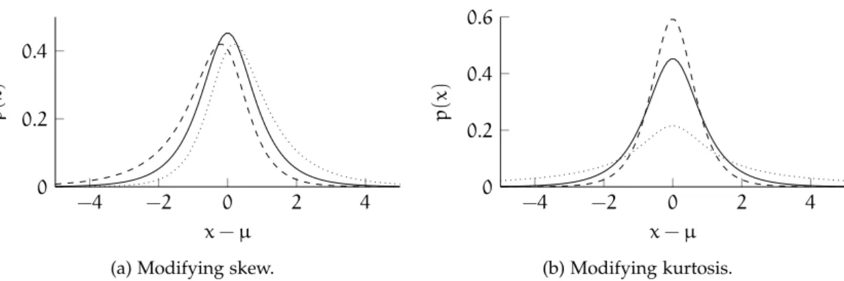
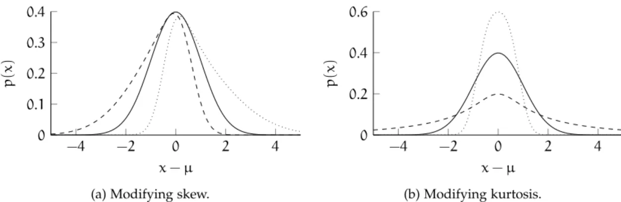
Figure 3.1 Normal and Student’s t-distribution . . . . 36

Figure 3.2 Generalised Hyperbolic distribution . . . . 37

Figure 3.3 Sinh-asinh distribution . . . . 38

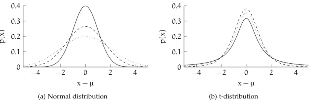
Figure 3.4 Gamma and beta distribution . . . . 40

Figure 3.5 Gaussian mixture model . . . . 44

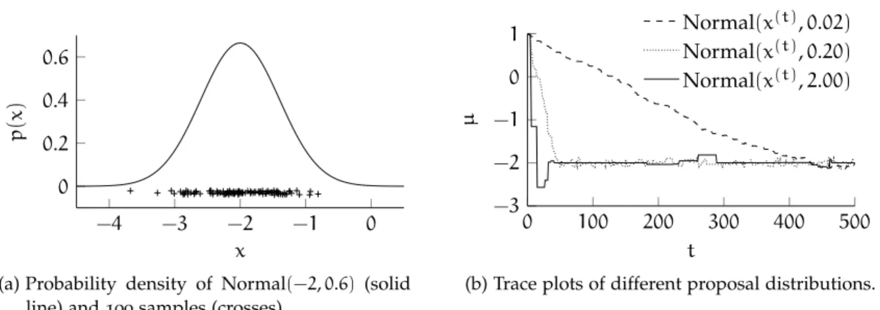
Figure 3.6 Influence of the proposal distribution in Metropoli-Hastings . . . 52

Figure 3.7 Distributions with different copula . . . . 57

Figure 4.1 Percentage of normally distributed marginal ground truth re- gions on the BSDS500 . . . . 63

Figure 4.2 Qualitative results on the BSDS500 for different colour spaces with and without positional features. . . . 64

Figure 4.3 Qualitative results of the analysed mixture models on the BSDS500 with a varying number of components. . . . 66

Figure 4.4 Qualitative results of the analysed mixture models on the BSDS500 with and without correlation included . . . . 69

Figure 4.5 Qualitative results of the tested mixture models on the BSDS500 . 74 Figure 5.1 Overview of the used feature channels . . . . 81

Figure 5.2 Relation between BIC and VoI for a sample image of the BSDS500 83 Figure 5.3 Qualitative results of the analysed methods to choose a number of mixture components . . . . 84

Figure 5.4 Visualisation of the idea to include edges as a part of the segmen- tation model . . . . 90

Figure 5.5 Visualization of the idea to include edges as a part of the segmen- tation model . . . . 92

Figure 5.6 Influence of choosing an appropriate mode for the beta distribu- tion of the edge model . . . . 93

Figure 5.7 Visualization of the quantities to build the Passive Edge Model . 94 Figure 5.8 Visualization of the idea to include edges as a part of the segmen- tation model . . . . 95

Figure 5.9 Qualitative results of the proposed edge models on the BSDS500 97 Figure 6.1 Overview of the proposed weakly supervised approach . . . . 104

Figure 6.2 Overview of the proposed Fully Convolutional Network architec- ture . . . . 107

Figure 6.3 Segmentation results on VOC segmentation task . . . . 110

Figure 6.4 Correct Localization results on VOC trainval split . . . . 112

xiv

L I S T O F TA B L E S

Table 4.1 Segmentation accuracies of a Gaussian Mixture Model in different colour spaces. . . . 65 Table 4.2 Comparision of different approaches for including positional in-

formation. . . . 67 Table 4.3 Segmentation accuracies of different types of probability distri-

butions including and excluding correlation . . . . 68 Table 4.4 Segmentation accuracies of different types of probability distri-

butions. . . . 72 Table 5.1 Comparison of four different strategies to reduce the computa-

tional burden. . . . 79 Table 5.2 Results of selecting an appropriate number of mixture compo-

nents on the BSDS500 . . . . 85 Table 5.3 Evaluation of the segmentation metrics of different algorithms on

the BSDS500 . . . . 91 Table 5.4 Evaluation of the proposed edge models on the BSDS500 . . . . . 98 Table 5.5 Comparison of the proposed segmentation models to state-of-the-

art approaches on the BSDS500 . . . . 99 Table 6.1 Accuracy on VOC segmentation task . . . . 111 Table 6.2 Correct Localization on VOC trainval split. . . . 113

xv

AIC Akaike Information Criterion AEM Active Edge Movement

BIC Bayesian Information Criterion BoF Bag-of-Features

BSDS500 Berkeley Segmentation Data Set and Benchmarks 500 [Arb+11]

BSDS300 Berkeley Segmentation Data Set and Benchmarks 300 [Mar+01]

cdf cumulative distribution function CorLoc Correct Localization

CNN Convolutional Neural Network DNN Deep Neural Network

DPMM Dirichlet Process Mixture Model DRAM Delayed Rejection Adaptive

Sampling

EM Expectation Maximisation FCN Fully Convolutional Network GMM Gaussian Mixture Model GP Gaussian Process

HoG Histogram of Oriented Gradients

IoU Intersection over Union KDE Kernel Density Estimation MCMC Markov chain Monte Carlo

MRF Markov Random Field MDS Multidimensional Scaling MTMM Multiple Scaled t-distribution

Mixture Model

OWT Oriented Watershed Transform PCA Principal Component Analysis PEM Passive Edge Model

pdf probability density function pmf probability mass function PRI Probabilistic Rand Index ReLU Rectified Linear Unit

RCNN Regional Convolutional Neural Network

SCMM Sinh-asinh Copula Mixture Model

SIFT Scale-invariant Feature Transform

SLIC Simple linear iterative clustering [Ach+12]

SVM Support Vector Machine UCM Ultrametric Contour Map VOC the PASCAL Visual Object

Classes Challenge 2012 [Eve+15]

VoI Variation of Information

xvi

N O TAT I O N A N D D E F I N I T I O N S

Mathematical Expressions

x

a scalar.

x

a vector.

X

a matrix.

X

a set.

f(x)

a function.

log(x) the natural logarithm.

p(x)

a probability density function.

P(x)

a cumulative distribution function.

x^T

,

the transposed.

n!

the factorial of a positive integer n.

(︁_n

k

)︁

the binomial coefficient.

|x|

the absolute value of a scalar.

||x||2

the euclidean norm of a vector.

x

¯ the mean of a vector.

x

˜ the median of a vector.

x_j

the j-th entry of the vector

x^(t)

,

,

,

a variable at time

X_i,j

the j-th entry of the i-th row of the matrix

X_i

the i-th row of the matrix

Xj

the j-th coloumn of the matrix

X_i

the i-th entry of the set

.

|X|

the cardinality of a set.

X ∪ Y

the union of the sets

and

X ∩ Y

the intersection of the sets

and

.

α

a shape parameter of a beta distribution.

β

a shape parameter of a beta distribution.

γ,γ

the asymmetry parameter of a generalized hyperbolic distribution.

Γ(x)

the gamma function.

δ,δ

the tail parameter of a sinh-asinh distribution.

xvii

ϵ,ϵ

the asymmetry parameter of a sinh-asinh distribution.

ζ

the concentration parameter of a Dirichlet distribution.

η

a tail parameter of a generalized hyperbolic distribution.

θ

a parameter of a probabilistic model, the quantity of interest.

Θ

the set of all parameters of a probabilistic model.

ι

the dispersion parameter of a Dirichlet process.

κ

the concentration parameter of a beta distribution.

λ,λ

an eigenvalue, the vector of all eigenvalues.

Λ

the diagonal matrix of all eigenvalues.

µ,µ

the mean value, the location parameter of a distribution.

ν,ν

degrees of freedom of a t-distribution/ multiple scaled t-distribution.

ξ

the acceptance pobability in a Metropolis-Hastings step.

ρ

the mode of a beta distribution.

σ,σ

the standard deviation, the scale parameter of a distribution.

σ²

the variance.

Σ

a covariance matrix.

τ,τ

the probability of success in a binomial/multinomial experiment.

ϕ_k(x)

the probability density function of the

mixture component in a mixture model.

φ(x)

the distribution function of a standard normal distribution.

φ⁻¹(x)

the quantile function of a standard normal distribution.

χ

a tail parameter of the generalized hyperbolic distribution.

ψ,ψ

an angle, a vector of angles.

ω,ω

the mixture weights of a mixture model.

Roman Symbols

1

the identity matrix.

a

the shape parameter of a gamma distribution.

A

the set of all class activation maps.

notation xix

A

a class activation map.

b

the scale parameter of a Gamma distribution.

b,B

the permutation index and the number of permuations used in a permutation test.

Bg

the background map used in deriving a semantic segmentation.

B

a boundary map derived from a segmentation.

c,C

the class index and the total number of classes.

C

a correlation matrix.

c(x)

the probability density function of a copula.

C(x)

the distribution function of a copula.

C(S → S^′)

the segmentation covering of two segmentations

and

.

i,D

the dimension index and the total number of dimensions.

E

the edge map of an image.

E[x]

the expectation value of a random variable

F

the F-measure.

F P

the set of all false positives in a binary classification.

F N

the set of all false negatives in a binary classification.

gx

,

the image gradient in x- and y-direction.

gt

a ground truth vector.

G(·)

a Dirichlet process.

G₀

the base distribution of a Dirichlet process.

G

a ground truth segmentation.

h

the bandwidth of a kernel function.

H(x)

the entropy of a discrete random variable.

H₀

the null hypothesis in a significance test.

H₁

the alternative hypothesis in a significance test.

H

the height of an image.

Iv(x)

the modified Bessel function of the first kind.

I

an image.

I(x,y)

the mutual information of two discrete random variables.

k,K

the cluster/mixture component index and the total number of clusters/mixture components.

Kv(x)

the modified Bessel function of the second kind.

k(x)

a kernel function.

l_ce

the cross-entropy loss.

L(θ)

the likelihood of a model.

L

a line segment of a boundary map.

L_seg

the set of all line segments of a boundary map.

m

the mean function of a Gaussian process.

M

the number of all free model paramters.

j,N

the instance index and the number of instances.

N⁺

the natural numbers excluding 0.

N_c

the number of colour channels.

N_R

the number of rotation matrices.

N_img

the number of pixels in an image.

N_s

the number of successes in a binomial experiment.

N_spx

the number of superpixels.

N_t

the number of trials in a binomial experiment.

P

a set of pairs of pixels.

Q

the matrix of transition probabilities of a Markov chain.

r_j,k

a binary cluster indicator set to true if the j-th instance belongs to the k-th cluster.

R

a region of a segmentation.

R

a rotation matrix.

R

the real numbers.

sd an estimate of the error induced by not using all possible permutations in a permutation test.

S

a segmentation.

T P

the set of all true positives in binary classification.

T(·)

a test statistic.

t

the vector of all computed test statistics in a permutation test.

t,T

a time index and the total duration.

u

the lower boundary of the uniform distribution.

v

the upper boundary of the uniform distribution.

V

the eigenvectors of a matrix.

W

the affinity matrix of a graph.

y

a class index.

y

ˆ the predicted class index.

z

a latent variable of a mixture model.

1

I N T R O D U C T I O N

Partitioning an image into coherent regions is an ongoing area of research in computer vision and the study of artificial intelligence in general. In contrast to scene or object recognition, not only the presence or absence of objects is predicted but also their full extent. In fact, every pixel in an image is classified. This enables us to know not only where an object appears but also to which extent an object occupies an image. This is, for instance, important when autonomous systems try to perceive their surroundings as in autonomous driving, when geologists build maps, or when physicists analyse medical images.

Nowadays, these problems are mostly solved with Deep Neural Networks (DNNs) like [RFB15; LSD15; BHC15]. However, such techniques impose some limitations as well.

For instance, they usually require a large amount of labelled training data [BV16a]. Ac- quiring them is especially challenging in the case of image segmentation because every pixel has to be annotated by a ground truth class. According to [Bea+16] annotating every pixel of an image takes roughly ten times longer (240 seconds compared to 20 seconds on average per image) than simply annotating the presence or absence of a set of object classes. The high effort makes creating datasets at best cumbersome, but mostly expensive. Another limitation of the DNN-based approach is the absence of use- ful uncertainty estimates, because the data are not modelled generatively, but only the decision boundary between classes is learned. This is a major drawback since the pre- diction of autonomous systems should be explainable. In fact, this is currently a major topic in politics and one of the central targets for artificial intelligence made in Europe

.

In this thesis, a contribution towards explainable artificial intelligence is made by fo- cussing on generatively modelling the observed data. This is achieved by utilizing a statistical concept termed mixture models. They are chosen because they offer uncertainty estimates through generatively modelling the observed data in the feature space with probability distributions. Essentially, the model does not only learn to decide but to accompany a decision with a probability which can be interpreted as a measure of con- fidence. Additionally, mixture models can directly be used in an unsupervised setting where the algorithms are only equipped with the raw data without any ground truth information. Mixture models then proceed at estimating the probability density func- tion (pdf) of the observed data by building a mixture of multiple probability distribu- tions. In this setting, it is assumed that every region is well described by one probability distribution.

In general, generatively modelling the data is harder than learning the decision bound- ary because the classes’ densities have to be learned as well. Naturally, this imposes several challenges, like the suitability of the data and the used probability distributions.

Further, in an unsupervised setting, the number of different regions in an image is a-

1 The European Commission’s high-level expert group on artificial intelligence, “Draft Ethics guidelines for trustworthy AI” https://ec.europa.eu/digital-single-market/en/news/

draft-ethics-guidelines-trustworthy-aiRetrieved June23,2020

1

priori unknown and has to be estimated. All these challenges are tackled in this thesis from a probabilistic perspective.

1.1 contribution

The contributions depicted in this thesis consist of three major parts. In the first part, the suitability of various probability distributions and image features are analysed in a supervised way. This successfully establishes an upper bound of the reachable segmen- tation accuracy. Additionally, a novel probability distribution is presented which shows an excellent performance. Using different distributions and their impacts are rigorously tested on predefined data sets and the impacts are assessed with statistical significance tests. The results have been previously presented in [WW16] and [WW17b]. This thesis additionally includes more probability distributions, an analysis regarding the used fea- tures, and an analysis regarding the expressiveness of various probability distributions.

In the second part, different ways to reduce the computational burden are examined and the mixture estimation is tackled from an unsupervised perspective. The major goal is to reach the previously defined upper bound. It is shown that one of the most limit- ing factors in an unsupervised estimation is the maximization of the model’s likelihood.

By including an additional model of the probable locations of region boundaries into the estimation, the performance is significantly increased. As a result, the gap between the upper bound and the unsupervised estimation is reduced. Again, the experiments are conducted on predefined data sets and accompanied by significance testing. The re- sults have been previously presented in [WW17a] and [WW17c]. This thesis additionally includes in-depth experiments regarding the estimation of the number of mixture com- ponents in the unsupervised setting. Further, previously unpublished results yielding the current state-of-the-art in generative image segmentation are presented.

Lastly, a probabilistic image model is combined with a DNN. The concept of class acti- vation maps is leveraged to get a generative segmentation model from a discriminatively trained DNN. The results have been previously presented in [Wil+17].

1.2 outline

Following the introduction, the remainder of this thesis is structured as follows: Chap- ter 2 reviews image segmentation from a general perspective, important terms and con- cepts are introduced, a review of different approaches is given, the benefits of generative models are discussed, and the requirements of a good segmentation model are defined.

Additionally, relevant data sets used throughout this thesis are presented. This is fol- lowed by an explanation of the segmentation metrics used in this thesis to quantitatively asses the quality of the segmentations.

Chapter 3 presents a concise summary of the relevant statistical concepts used in this

thesis. Beginning with an explanation of the Bayesian paradigm, different probability

distributions are introduced. Further, Markov chain Monte Carlo (MCMC) is explained

and significance testing in the context of image segmentation is briefly discussed. Build-

ing on the previously introduced concepts, the suitability of various probability distribu-

tions in the context of image segmentation is analysed in Chapter 4. The novel Sinh-asinh

Copula Mixture Model (SCMM) is introduced and the upper bound of the segmentation

1.2 outline 3

metrics of various probability distributions are computed. While the estimation of the

upper bound has been conducted in a supervised fashion, in Chapter 5 the best way to

reach the upper bound in an unsupervised way are examined. Afterwards, the gained

knowledge about generative image segmentation is used in Chapter 6 to build a gen-

erative segmentation model from a discriminatively trained DNN. The experiments are

conducted in the challenging weakly supervised setting. In the last chapter the results

are summarized and possible future research directions are sketched.

2

I M A G E S E G M E N TAT I O N

The goal of image segmentation is to divide an image into regions. Each region is a set of pixels which share a specific trait. Depending on the analysed images these traits can vary. Typical traits are, among others, colour (e. g., [CM02]), texture (e. g., [JF91]), or semantic meaning (e. g., [Eve+15]).

Image segmentation is, for instance, applied in autonomous driving (e. g., [Cor+16]).

The car needs to perceive its surroundings accurately in order to drive safely. One part of this perception is to know the extents of all occurring objects in the car’s field of view.

Typical objects which appear in a street scene are, among others, cars, persons, or street signs. In terms of image segmentation, the goal is to automatically divide the pixels of an image into disjoint sets where each region includes only one type of object. For instance, all pixels which depict a car are grouped into one region.

Creating maps is also a similar task. Like geologists build maps from remotely sensed data, image segmentation algorithms build regions from analysing the provided data (see e. g., [Zhu+17]). Depending on the features these results may differ and depending on which model is used the interpretation changes. Another example of image seg- mentation in practice is assisting physicians in analysing medical image data (see e. g., [Lit+17]) where they are trying to detect anomalies in the sizes of cells or organs. In every case, every pixel of an image needs to be given a label which indicates the re- gion membership. Despite the possible semantic interpretation of a region, the question arises what is a good segmentation and how can it be defined. This is especially relevant if a semantic interpretation is not directly available or desired. In the literature, several properties are listed which characterize a good segmentation. For instance, according to [HP17] a segmentation of an image should have:

1. uniform and homogeneous regions according to some criterion, 2. significantly different adjacent regions,

3. simple regions without holes, 4. simple and accurate boundaries.

In image segmentation, a boundary is the set of pixels which have more than one region in its direct vicinity. While all these properties are worth following, in this thesis, two additional goals are followed. A segmentation should additionally have:

5. sensible uncertainty estimates,

6. been computed with an as small amount of expert knowledge as possible.

One of the major goals of this thesis is to additionally provide meaningful uncertainty measures regarding the affinity with which pixels belong to the regions of an image.

This is a helpful tool when communicating segmentation results to domain experts, like physicians in medical image analysis or geologists in remote sensing applications.

5

Another key aspect is to develop methods which solve the image segmentation prob- lem by using as few human annotations as possible. This is important because acquiring human annotations is at best cumbersome but mostly expensive. For instance, accord- ing to [Bea+16] annotating every pixel of an image takes roughly ten times longer than simply stating if an object is present or not. When creating annotations of everyday scenes this work can be crowdsourced (e. g., [Rus+15]) or brought by citizen scientists (e. g., [Swa+15]). However, in other fields, like medical image analysis or when analysing remotely sensed surfaces of planets, domain experts are needed to annotate data.

This chapter starts with a short treatise of the fundamentals of probability theory in Section 2.1 because the remainder of this thesis heavily relies on it. Depending on the used data (see Section 2.2), image segmentation can be done with the help of different levels of supervision (see Section 2.3). In Section 2.4 model-based approaches are re- viewed in the context of image segmentation. Distance-based approaches are reviewed in Section 2.5, and approaches based on detecting contours in Section 2.6. This is fol- lowed by a small treatise of superpixels (see Section 2.7), which can be considered as a special case of image segmentation. Semantic segmentation, which is another special case of image segmentation, and Deep Neural Networks (DNNs) are discussed in Sec- tion 2.8. Afterwards, scene and object detection tasks (see Section 2.9) and segmentation tasks (see Section 2.10) are presented. The chapter concludes with a discussion of com- mon evaluation metrics used in image segmentation (see Section 2.11).

2.1 fundamentals of probability theory

Probabilities are a key concept in machine learning in general and in image segmen- tation in particular. In this section, the elementary notations and concepts are briefly introduced. Detailed introductions can, among others, be found in [Bis06; Mur12; BH14].

Following [Ly+17], a statistical model is a function

xi|θ)︁

which relates the potential outcomes

of a random variable

through a set of parameters

comes are elements of an output space

which is the set of all possible events or values the random variable can take. If

is a finite set of discrete events, like the result of a coin toss, the random variable

is termed discrete. Further, the function

x_i|θ)︁

is known as the probability mass function (pmf). In Section 3.2.1, some commonly used pmfs are presented. If

is continuous, the random variable

is termed continuous and

is known as the probability density function (pdf). In Section 3.2, relevant pdfs used in this thesis are presented.

The probability of observing the outcomes of two random variables together is known as the joint probability of

and

denoted by

thrown simultaneously. The joint probability of both dice is then the Cartesian product of the respective sample spaces [BH14, p. 545]. Commonly, this is visualized as a matrix representation of all possible outcomes. However, all combinations are equally probable, because the two dice are unconditionally independent [Mur12, p. 30], that is, one die does not influence the outcome of the other. Formally, this is expressed as

p(x,y) =p(x)·p(y).

(2.1)

If, however, the two random variables are not independent, this simplification is not

valid. The concept of conditional probability, denoted by

2.1 fundamentals of probability theory 7

of a random variable

after another random variable

has been observed first. It is defined through the joint probability of

and

occurring together and the probability of

alone and computed as [Mur12, p. 29]

p(x|y) = p(x,y)

p(y)

. (2.2)

In the case of continuous random variables, the probability that a value x lies in an interval

is computed as [Bis06, p. 17]

p(x∈(a,b)) =

∫︂_b

a

p(x)dx

(2.3)

with

as the pdf. Since probabilities are always non-negative, the following two conditions have to be met such that

is a valid probability distribution [Bis06, p. 18].

p(x)⩾0,

(2.4)

∫︂_∞

−∞p(x)dx=1.

(2.5)

The first condition simply enforces that probabilities cannot be negative, and the second condition enforces that the chance of observing

somewhere on the real line is always true. Actually, the relation in Equation 2.3 is used to define the cumulative distribution function (cdf) of a random variable and is defined as [Mur12, p. 32]

P(z) =

∫︂_z

−∞p(x)dx.

(2.6)

Further,

is the derivative of

probable it is to observe an outcome which exceeds a certain value. This is, for instance, important when using the cdf in conjunction with a copula [Nel06]. In this thesis, copulas are used to derive a highly flexible class of multivariate distributions which show an excellent performance at image segmentation. See Section 3.6 and Chapter 4 for further details.

Another important aspect of this thesis is Bayes’ law [Bay63] and the implications of interpreting it as a sensible way to tackle image segmentation in a fully probabilistic way. In general, Bayes’ law is a simple result of the foundations of probability theory, also known as Kolmogorov axioms (see [Fah+07, p. 182]), and the rules of probability derived from them (see [Fah+07, p. 185]). However, the law which was credited to the reverend Thomas Bayes has been discovered before Kolmogorov set out the foundations of probability theory. Bayes’ law is expressed in the continuous case through several probability distributions as [Gel+13, p. 7]:

p(θ|x) = p(θ,x)

p(x) = p(x|θ)p(θ)

p(x) = ∫︁ p(x|θ)p(θ)

θp(x|θ)p(θ)dθ

, (2.7)

with

as the model parameters,

as the posterior,

as the likelihood,

as

the prior, and

as the evidence [Bis06, p. 22]. The posterior distribution is the ultimate

result of the analysis. It is a probability distribution over the parameters of the model

conditional on the observed data. The likelihood describes the model which is fitted to

the data.

Note that the posterior is, in contrast to the likelihood, conditioned on the data. There- fore, it expresses the uncertainty of the parameters conditioned on the observed data.

The likelihood is defined conversely and quantifies the uncertainty of the data condi- tional on the parameters. However, this is not the quantity we are interested in. We are interested in quantifying the uncertainty with which we have estimated the parameters of our model and this can only be assessed by consulting the posterior distribution. This fundamental change of perspective is a key feature of Bayesian statistics.

In this thesis, several probability distributions are used to describe the observed im- age as well as possible. Each model consists of of parameters

and the prior belief of the model parameters is expressed through the prior. An in-depth review of prior dis- tributions and the implications of using them in a Bayesian framework are discussed in Section 3.1. Finally, the evidence is the probability of observing the data

is usually no sensible way to compute this quantity, it is commonly rewritten as an inte- gral over the parameters

of the joint probability distribution. As a result, closed form expression for the posterior can only be given analytically if certain conditions are met (see Section 3.1). Otherwise, the computation of the evidence is intractable and samples of the posterior have to be drawn. One powerful class of methods for drawing samples from arbitrary probability distributions is Markov chain Monte Carlo (MCMC) which is explained in Section 3.4.

2.2 the data

Image segmentation is a special case of pattern recognition. The goal is to find patterns in image data by looking at local similarities and grouping pixels into regions. The data themselves consist of instances [Zhu+09, p. 2]. In a general setting, an instance is, for example, one specific animal. It can be described by its characteristics, like height and size, or, as shown later, by a photograph. Formally, one instance

of the data is a representation of one specific object. It is represented by a

,

,

,

. Each element of this vector is termed a feature of the instance [Zhu+09, p. 2]. Depending on the problem domain these features are measured, like height or weight, or they are derived from measurements, like the body mass index.

In this work, the measurements are images which have been captured by a photogra- pher. Therefore, the measurements are matrices instead of vectors. One instance of the data is an image

which consists of a set of colour channels. Formally this is expressed as

I¹

,

,

. Each channel has the same size as the others. One colour channel

of the size

equals

I^c =

⎡

⎢⎢

⎢⎢

⎢⎣

x^c_1,1 x^c_1,2 . . . x^c_1,W x^c_2,1 x^c_2,2 . . . x^c_2,W

... ... ... ...

x^c_H,1 x^c_H,2 . . . x^c_H,W

⎤

⎥⎥

⎥⎥

⎥⎦

with

as the height and

as the width of an image. Commonly, an image consists of

three colour channels

which represent the intensity of the captured light in

the red, green, and blue wavelengths.

2.2 the data 9

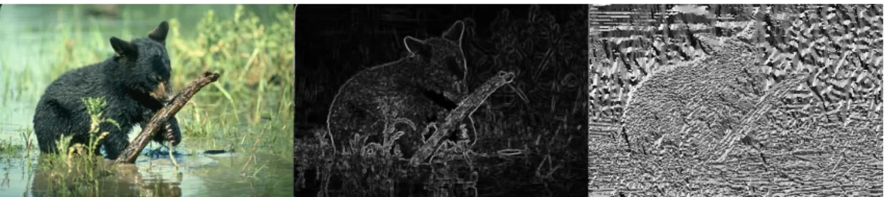
Figure2.1: Image of a bear cub (left), the corresponding gradient magnitude (middle), and gra- dient orientation (right). Image taken from the Berkeley Segmentation Data Set and Benchmarks500[Arb+11].

The CIE 1976 L*a*b* Colour space (Lab) [Rob77] is an often used alternative to the RGB colour space. Colours in Lab are computed through a nonlinear transformation of the RGB colour space. The key idea behind Lab is to better resemble the human perception of colour, that is, colour differences perceived by humans behave similar to distances in the Euclidean space. Colour spaces which exhibit this property are termed perceptually uniform. See, for instance, [Pas01] for an overview of common colour spaces and a performance evaluation of images in different colour spaces in a supervised clas- sification setting. While in [Pas01] the Hue Saturation Value (HSV) colour space (see, e. g., [GW02, pp. 295-301]) performs best, Lab and RGB are almost exclusively used in image segmentation. In Chapter 4 different colour spaces are analysed regarding their suitability in image segmentation tasks and the question if perceptually uniform spaces are better at image segmentation is tried to be answered. In a recent study, [GY19] con- ducted an analysis where the influence of choosing different colour spaces on DNNs is studied.

Besides colour alone, a plethora of image features exist in computer vision. The most famous variants are probably the Scale-invariant Feature Transform (SIFT) descriptor [Low99] and the Histogram of Oriented Gradients (HoG) descriptor [DT05]. Both meth- ods are based on gradients [GW02, p. 577]. They look at a local area around an interest point inside the image, termed image patch, and examine the orientations of the gradi- ents in this area. Computing the gradients of an image can be interpreted as a simple version of edge detection. In Chapter 5 an edge detector plays an important role when increasing the quality of the computed segmentations. Formally, the image gradient is the derivative of a real multivariate function

in

and

dimension.

∇f= [︄g_x

gy

]︄

= [︄∂f

∂x

∂f

∂y

]︄

In practice, the real multivariate function

is the image

. Since an image commonly consists of multiple colour channels, it is converted to greyscale first. Afterwards, the gradient is approximated numerically by finite differences. The orientation and the mag- nitude of the gradient at a given pixel are then calculated as [GW02, p. 577]

orientation

tan

g_x )︃

, magnitude

g²_x+g²_y

.

HoG and SIFT then proceed by quantizing the gradient information inside an image

patch around a query point into a histogram representation. The query point at which

Figure2.2: Visualization of the48filters used in [LM01] for recognizing different textures. The filter bank consists of first and second order Gaussian derivatives at six orientations and three scales, eight Laplacian of Gaussian filters, and four Gaussian filters.

this descriptor is computed can be estimated from potentially relevant key points, as in the original SIFT paper [Low99], or they may be extracted on a dense grid, for instance at every n-th pixel [BZM06]. This approach is also known as Dense SIFT.

A single image is thus described by a possibly large set of descriptors. This represen- tation can then be used to infer the scene of an image or to detect the objects which are present in an image. In the original SIFT paper, this amounts to a 128-dimensional feature vector per key point. A possible extension of this is the Bag-of-Features (BoF) approach, where a visual codebook is generated by clustering a large set of descriptors from a large set of images. The key idea behind the BoF approach is to find a codebook which consists of discriminative descriptors. An image can then be described by a his- togram of the occurrences of the codebook entries. While this approach originates from the Bag-of-Words model used in document analysis, it is successfully applied in image and scene classification tasks [FFP05; LSP06; OD11].

While the Bag-of-Words model can be considered as a precursor of the BoF approach, the idea to create a histogram representation through clustering was previously intro- duced in [Sch01] as an approach to image retrieval and in [LM01] as a way to discrimi- nate between images with different textures. The latter name their approach textons. The main difference between BoF and the texton approach are the features which are clus- tered to form the codebook. Textons are computed by convolving the image with a filter bank and clustering the computed responses [LM01]. The used filter bank consists of a set of Gabor filters [FS89], which have a long tradition in texture recognition. These filters respond to different spatial frequencies like edges or stripe patterns. Commonly, filter banks not only consist of Gabor filters, but also of Gaussian filters. Additionally, their first and second derivatives are used. The primary goal of the Gaussian filters is having high responses at image structures which are not edges. Figure 2.2 depicts a typical filter bank used for recognizing images with different textures [LM01]. Due to their success- ful application in texture recognition, the use of textons has been extensively studied in image segmentation tasks as well [JF91; Mal+99; SJC08; Arb+11].

2.3 levels of supervision

Image segmentation can be formulated as a machine learning problem. In machine learn- ing, different levels of supervision are distinguished in order to describe how much information the human expert provides such that algorithms learn to solve a problem.

Conversely, different levels of supervision are necessary depending on the chosen algo-

2.3 levels of supervision 11

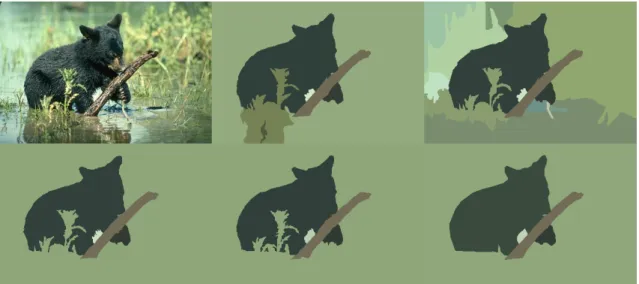
Figure2.3: Image of a bear cub (top left) and the corresponding ground truth annotations. The ground truth images are colour coded by the mean RGB value of the correspond- ing regions. While the similarities across different annotations are evident, they vary strongly in the level of abstraction, especially in the background. Images taken from the Berkeley Segmentation Data Set and Benchmarks500[Arb+11].

rithm. Estimating the parameters of a model is also known as learning [Bis06, p. 2]. In this thesis, four levels of supervision are distinguished: supervised learning, unsupervised learning, semi-supervised learning, and weakly-supervised learning.

The image segmentation problem can be learned in a fully supervised framework, where each instance of a set of images is accompanied by a labelled ground truth im- age. It is of the same size as the training image and each pixel is annotated with the desired prediction of the algorithm. They are the associated classes or objects visible in an image. Figure 2.3 provides a sample from the Berkeley Segmentation Data Set and Benchmarks 500 [Arb+11] (BSDS500) and depicts how different annotators perceive the regions of an image differently. This illustrates that there is sometimes not one single correct solution, but often a set of probable solutions. In this thesis, we tackle this issue by modelling the number of regions probabilistically (see Section 3.5.1 and Chapter 5).

2.3.1 Unsupervised Learning

This thesis deals mainly with approaches to unsupervised learning and how these can be used to solve the image segmentation problem. In general, unsupervised learning is concerned with describing the structure of the data and how different features or instances are grouped in the feature space without using any expert knowledge.

Formally, we are working with a set of instances

,

,

and try to build models which resemble the unknown generating distribution as closely as possible.

Therefore, the models are of the form

as the set of model parameters.

Each

is assumed to be drawn i. i. d. (independently and identically distributed) [Bis06,

p. 26] from an unknown generating distribution. Assuming i. i. d. instances is of great

importance because this enables us to independently evaluate the likelihood of all in-

stances. This means that we can neglect possible correlations among the instances and

evaluate the likelihood of multiple instances as a product of the likelihoods of the sin- gle instances. Formally, the likelihood of

instances conditioned on a set of model parameters can be expressed as [Bis06, p. 26]:

p(X|θ) =

∏︂N j=1

p(︁

x_j|θ)︁

. (2.8)

The independence assumption is of central importance for many machine learning al- gorithms. For instance, predictions about previously unseen instances would not be possible without it [GBC16, p. 109]. However, the independence assumption is rather limiting in practice, because one can easily assume cases where instances are correlated.

Algorithms which are especially suited for unsupervised image segmentation are pre- sented in Section 2.4. They include, among others, the well-known Gaussian Mixture Model (GMM). Further details about mixture models are presented in Section 3.2.4.

2.3.2 Supervised Learning

Unlike unsupervised learning, supervised learning uses additional information. Every instance

of the data is accompanied by a desired prediction

which is also known as a label or ground truth. In the case of a continuous desired prediction, the problem is termed a regression. In the case of a discrete desired prediction

, the problem is termed a classification. In both cases, the set of instances

is accompanied by a set of desired predictions

,

,

which are assumed to be drawn from a joint probability distribution

The goal of parameter inference is to learn a model which predicts the correct label given an instance. Therefore, the model is not only conditioned on the parameters of the model, as in Equation 2.8, but also on the instances

. In a generative framework for classification, Bayes’ theorem (see Section 2.1) is used to condition the joint probability distribution

,

on the

labels and estimate the respective density [Bar12, p. 300]:

p(y_j|xj

,

,

∑︁_C

c=1p(x_j

,

,

∑︁_C

c=1p(x_j|c,θ)p(c|θ)

. (2.9) This approach explicitly models the generation of an instance through

,

Chapter 6 this relation will be used to compute a semantic segmentation. Again, i. i. d. instances are assumed such that the relation for all instances can be expressed as

p(Y|X

,

∏︂N j=1

p(y_j|xj

,

(2.10)

Equation 2.10 expresses supervised learning from a probabilistic perspective. However,

it is sufficient to learn a function

which maps the observed instances to the desired

predictions. Formally, this relation is expressed as

. Often, this mapping is

done by dividing the feature space into cells. The boundaries of the cells are described

by classifiers, like the Support Vector Machine [CV95] or a neural network (see Sec-

tion 2.8.1). As a result, discriminative approaches model the boundaries between classes

2.3 levels of supervision 13

and generative approaches model the distribution of the different classes in the feature space. While a generative model is more complex than a discriminative model, it allows the computation of uncertainty estimates.

Unlike unsupervised learning, supervised learning is more about predicting than ex- plaining the data generation process. Further, supervised learning makes use of labelled instances explicitly. If those labels are available, supervised algorithms are supposed to yield better results in terms of prediction accuracy. However, the labels need to be acquired somehow in practice. Depending on the type of problem, this comes with ex- ceptional human effort. For instance, in the case of image segmentation every single pixel has to be annotated by an expert. Depending on the problem domain even finding suitable experts is challenging.

2.3.3 Semi-Supervised Learning

Semi-supervised learning is the bridge between supervised and unsupervised learning.

Instead of having a label for every instance, as in supervised learning, only a subset of all instances is annotated. Methods from the semi-supervised learning literature use the unlabelled data to improve supervised learning on the available subset of labelled instances.

Formally, the set of all instances

consists of a set of unlabelled instances

,

,

and a set of labelled instances

,

,

edge about

can be used to improve the model of the labelled instances

both sets are used during training. For instance, in a generative framework (cf. Equa- tion 2.9) this knowledge can be directly incorporated into the estimation of a GMM [Zhu+09, pp. 25-28]. Semi-supervised learning is especially well suited if numerous in- stances are available, but labelling is tedious or expensive.

In terms of image segmentation, semi-supervised learning can be done by partially annotating an image by an expert. For instance by painting brush strokes, called scribbles (see e. g., [Lin+16; HKH17]), or by annotating single points in an image [Bea+16]. Then, the algorithm does not only know how many regions the expert expects but is also equipped with a first set of labelled instances

.

2.3.4 Weakly-Supervised Learning

In computer vision, weakly supervised methods are concerned with recovering the ex- tent of an object by only knowing the presence or absence of an object in an image [HKH17]. Especially in image segmentation, acquiring annotated ground truth data is cumbersome [Bea+16; Cor+16], because every single pixel needs to be annotated by a hu- man expert. One way of reducing the annotation effort is by asking experts to annotate only parts of an image, as in semi-supervised learning. Another approach is to increase the annotation’s level of abstraction. Instead of annotating at pixel-level, the images are annotated at image-level. For instance, the image is then only annotated by keywords.

The exact extent of an object inside an image, as in supervised learning, is not part of

the annotation and thus remains unknown to the algorithm. This significantly increases

the complexity of the learning problem, because the algorithm needs to derive the look

and shape of objects on its own. Further, it needs to learn common features of, for ex-

ample, persons without knowing how persons look like or where to find them in an image. Commonly, DNNs are used for this kind of tasks [HKH17]. They learn these re- lations from a large collection of training images. An overview of current approaches in weakly-supervised image segmentation is presented, for instance, in [HKH17]. In Chap- ter 6 a generative approach towards weakly supervised object detection and semantic segmentation is presented.

2.4 model- based approaches

Assuming a model for the data is one approach to image segmentation. In the context of colour images, this means that each region of an image is associated with a specific colour or distribution of colours. However, this neglects the spatial arrangement of the pixels inside an image. Pixels in close vicinity should have a higher probability to be- long to the same class. Therefore, the

as additional features [CM02] or, as suggested in the related work, modelled as well [SNG08]. In the following, several model-based approaches are presented and reviewed in the context of their use of labelled data.

2.4.1 Thresholding

One of the simplest approaches to segment a greyscale image into a set of regions is thresholding [Sze10, p. 284]. A user defines the levels at which the regions are separated by observing how adjusting the thresholds change the segmentation until a satisfactory result is achieved. In terms of the previous section, this is a supervised approach. How- ever, a rather simple model is used.

Since determining suitable thresholds for a collection of images is tedious, algorithms exist which return suitable thresholds based on some criteria. Among others, Otsu’s method [Ots79] is one of the commonly used methods. It determines suitable thresh- olds by looking at the variance of the values inside the regions. If this intra-class variance is minimal the optimal thresholds are reached. This follows the assumption that each region is associated with a unique mode of the histogram. In principle, Otsu’s method computes the parameters of a one-dimensional GMM (see Section 3.2.4) by exhaustively searching for the combination which minimizes the intra-class variance of the compo- nents.

However, Otsu’s method was developed for thresholding greyscale images. Although thresholds for every colour channel can be computed, this neglects the common appear- ance of data points in the feature space, because each dimension is treated indepen- dently of the others. An approach to respect common appearances in the feature space, is partitioning the feature space by solving the K-means problem.

2.4.2 K-Means Clustering

Originating from the clustering literature, solving the K-means problem has a long tradi-

tion in many scientific fields [Jai10]. Lloyd’s algorithm [Llo82], better known as K-means

clustering, is the typical approach for solving the K-means problem. While K-means

clustering is an unsupervised algorithm, it is limited to finding spherical groups in the