New concepts of multiple tests and their use for evaluating high-dimensional EEG data
Claudia Hemmelmann
a,∗, Manfred Horn
a, Thomas S¨usse
a, R¨udiger Vollandt
a, Sabine Weiss
b,caInstitute of Medical Statistics, Computer Sciences and Documentation, University of Jena, D-07740 Jena, Germany
bSFB360, University of Bielefeld, Germany
cBrain Research Institute, Cognitive Neuroscience Group, Medical University of Vienna, Austria Received 30 April 2004; received in revised form 12 August 2004; accepted 18 August 2004
Abstract
Recently, new concepts of type I error control in multiple comparisons have been proposed, in addition to FWE and FDR control. We introduce these criteria and investigate in simulations how the powers of corresponding test procedures for multiple endpoints depend on various quantities such as number and correlation of endpoints, percentage of false hypotheses, etc. We applied the different multiple tests to EEG coherence data. We compared the memory encoding of subsequently recalled and not recalled nouns. The results show that subsequently recalled nouns elicited significantly higher coherence than not recalled ones.
© 2004 Elsevier B.V. All rights reserved.
Keywords: Coherence; EEG data; FDR control; FWE control; Multiple endpoints; Multiple test; Permutation test; Power of test
1. Introduction
Modern procedures of EEG analysis yield large sets of high-dimensional parameters, which have to be evaluated statistically. Let k denote the dimension of the observations.
This means there are k components, which are also called multiple endpoints. InHemmelmann et al. (2004)we dealt with so-called global tests or multivariate tests which pro- vide one joint statement on all k endpoints. We now consider procedures that provide a statement for each endpoint. Many authors use anα-level test for each single component or end- point of the observational vector, see e.g.Rappelsberger and Petsche (1988). However, this practice results in a large num- ber of false positive statements (false discoveries, type I er- rors). There exist several techniques to cope with this general drawback in multiple comparisons. Corresponding multiple tests will be considered in the present paper.
Our paper has the following aims: (a) to introduce both traditional and recently proposed concepts of error control in
∗Corresponding author. Tel.: +49 3641 9 33610; fax: +49 3641 9 33200.
E-mail address: hemmel@imsid.uni-jena.de (C. Hemmelmann).
multiple comparisons, (b) to investigate corresponding multi- ple test procedures regarding their dependence on the dimen- sion k, the fraction of false hypotheses and the correlation structure of the data and compare the powers of different methods, and (c) to demonstrate the use of different multi- ple tests in problems of multiple comparisons of coherence values obtained from EEG data recorded during the memory encoding of subsequently recalled or not recalled abstract nouns (Weiss et al., 2000).
The techniques we discuss are not specific to EEG data;
they are equally applicable to the large data in MEG and fMRI.
2. Methods
2.1. Multiple tests and type I error control
As explained inSection 1, our observations are vectors of dimension k. Assume we have to compare paired sam- ples or two independent samples. Let x = (x1,. . ., xk) and y = (y1, . . ., yk) denote the corresponding random vec-
0165-0270/$ – see front matter © 2004 Elsevier B.V. All rights reserved.
doi:10.1016/j.jneumeth.2004.08.008
Table 1
List of methods considered in this paper
Method Abbreviation Requirement
Bonferroni method Bonf
Step-down procedure ofHolm (1979) Holm P(V > 0)≤α
Step-down procedure ofTroendle (1995) Troe
Step-up procedure ofBenjamini and Hochberg (1995) BH
Two-stage procedure ofBenjamini et al. (2001) BKY E(Q)≤α
Step-down procedure ofBenjamini and Liu (1999) BL99
Step-down procedure ofBenjamini and Liu (2001) BL01
Step-down procedure A ofKorn et al. (in press) PrAu P(V > u)≤α(0≤u < k)
Step-down procedure B ofKorn et al. (in press) PrB␥ P(Q >γ)≤α(0 <γ< 1)
tors and (µx1, . . . , µxk) and (µy1, . . . , µyk) the respective means. Then, the individual null hypotheses to be tested are H1:µx1 =µy1, . . . , Hk:µxk =µyk. Tests forH1, . . . , Hk
are called multiple tests.
It can happen that one of the k hypotheses, say Hi, is re- jected though it is true. Such an event is called type I error or false discovery. Let R denote the random number of re- jected hypotheses and V the random number of rejected true hypotheses, i.e. type I errors (V ≤ R ≤ k). An interesting quantity is the fraction V/R of falsely rejected hypotheses.
As this is not defined for R = 0, we introduce a new random variable Q where Q = V/R if R > 0 and Q = 0 if R = 0. In the literature, Q is called false discovery proportion whereas the expectation E(Q) is called false discovery rate (FDR).
Different concepts of controlling the proportion or the num- ber of false discoveries have been proposed, together with corresponding methods which control these rates in multiple testing problems. In the next sections, we will present and compare the test procedures listed inTable 1which satisfy four different criteria that are defined by the requirements given in the last column.
2.1.1. Control of the FWE
As already mentioned inSection 1, it is not advisable to use an α-level test for each of the k hypotheses, i.e. a test that rejects a true hypothesis with probabilityα, because in this case the expected number of false discoveries E(V) may be rather large; in the worst case, it can be as high as kα. And the probability FWE = P(V > 0), i.e. the probability of committing at least one type I error may also be very large, especially when k is large. FWE is the abbreviation of the term familywise error rate. For multiple comparisons it has been long recommended to use test procedures that control the FWE, i.e. that guarantee that FWE≤αno matter how many and which hypotheses are true.αis a prespecified small probability.
The simplest way to ensure that FWE≤ αis to test all individual hypotheses H1,. . ., Hk at levelα/k. This is the well-known Bonferroni method (Bonf). Assume we use some parametric or nonparametric test appropriate for H1,. . ., Hk, e.g. the t-test and obtain the p-values p1,. . ., pk. Then, Bonf rejects Hiif pi≤α/k.
Another simple method is the step-down procedure of Holm (1979)(Holm). Let p(1) ≤ · · · ≤p(k) denote the or- dered piand H(1),. . ., H(k)the corresponding hypotheses. In the first step, p(1)is compared withα/k. If p(1)>α/k, none of the k hypotheses will be rejected and the procedure stops. If p(1)≤α/k, H(1)is rejected. Then p(2)is compared withα/(k− 1). If p(2)>α/(k−1), H(2),. . ., H(k)are accepted. Otherwise H(2) will be rejected, etc. Clearly, Holm rejects at least all hypotheses that are rejected by Bonf. This means, Holm is more powerful.
Bonf and Holm do not take into consideration the correla- tion between the endpoints. In contrast, the step-down method ofTroendle (1995)(Troe) is adaptive to data correlations be- cause it is a permutation method. Similar to Holm, it is based on the ordered p-values p(1)≤ · · · ≤p(k). Choose B−1 ran- dom permutations of the data vectors consistent with the ex- perimental design. Denote the univariate p-values for the vari- ables from the jth permutation bypj1, . . . , pjkfor j = 1,. . ., B− 1, wherepj1corresponds to H(1),pj2to H(2), etc. Therefore, pj1, . . . , pjk are not ordered. Let pjmin,1=min{pj1, . . . , pjk} for j = 1,. . ., B−1. In the first step, p(1)is compared with theα-quantile of the B p-valuesp(1), p1min,1, . . . , pB−min1,1. If p(1) is larger than thisα-quantile, none of the k hypotheses will be rejected and the procedure stops. If p(1) is smaller than or equal to thisα-quantile, H(1) is rejected. Then omit all p-values corresponding to H(1), i.e.p(1), p11, . . . , pB−1 1. Now, let pjmin,2=min{pj2, . . . , pjk} for j = 1, . . ., B − 1.
Then p(2)is compared with theα-quantile of the B p-values p(2), p1min,2, . . . , pB−min1,2. If p(2)is larger than thisα-quantile, H(2),. . ., H(k)are accepted and the procedure stops. Other- wise H(2)will be rejected, etc.
As already mentioned inTroendle (1995), Troe is identical with the method ofWestfall and Young (1993). We will see that the power of Troe is higher than the power of Holm in many cases.
Holm and Troe (and Bonf inSection 3.3) are the only FWE controlling methods that we consider in this paper. However, there exist many other ones. A step-up analogue of Holm was proposed byHochberg (1988). It compares the p-values p(i)in the reverse order with the same critical bounds, i.e., in the first step p(k) withα, in the second step p(k−1) with
α/2,. . ., in the last step p(1) withα/k. However, Hochberg’s method is only valid under independence of the test statistics or at least under positive regression dependency which is a very general statement of a nonnegative correlation structure, seeSarkar (1998). In many-one comparisons by Horn and Dunnett (2004)the powers of Hochberg’s method and Holm did not essentially differ. Thus, we did not include Hochberg’s procedure in our investigations.
Many FWE controlling methods and techniques were de- scribed in the monographs ofHochberg and Tamhane (1987) andWestfall et al. (1999). A further interesting type of FWE controlling procedures was proposed byL¨auter (1997),Kropf (2000)andKropf et al. (2004). This approach uses a data driven order of the hypotheses.
2.1.2. Control of the FDR
The requirement FWE≤αis equivalent to P(V = 0)≥1− α. This means one requires that with large probability no true hypothesis is rejected no matter how large k is. In problems with large k, this requirement appears to be too strict. Thus, Benjamini and Hochberg (1995)introduced a new criterion which requires FDR = E(Q) = E(V/R|R > 0) P(R > 0)≤α. For example, FDR≤0.05 roughly means that on average no more than 5 of 100 significance statements are type I errors.
The control of the FDR in the evaluation of EEG data has already been proposed byDurka et al. (2004).
Benjamini and Hochberg (1995)were the first who pro- posed a test procedure (BH) that controls the FDR. Similar to Holm, it is based on the ordered p-values p(1)≤ · · · ≤p(k) obtained with some parametric or nonparametric test appro- priate for H(1),. . ., H(k). However, BH is a step-up procedure.
In the first step, p(k)is compared withα. If p(k)≤α, all hy- potheses are rejected. If p(k) > α, H(k) cannot be rejected.
Then p(k−1) is compared withα(k−1)/k. If p(k−1) ≤α(k
−1)/k, H(k−1),. . ., H(1) are rejected. If p(k−1) >α(k−1)/k, H(k−1)cannot be rejected, etc.
Let m denote the unknown number of false and k–m the number of true hypotheses.Benjamini and Hochberg (1995) have shown that for their procedure FDR≤α(k−m)/k. Thus, FDR is smaller thanαif m > 0 and decreasing with increasing m. If m were known one could increase the power of this step- up procedure by usingα=α∗·k/(k−m) instead ofα. Based on this idea,Benjamini et al. (2001)developed a two stage procedure (BKY). In the first stage, BH is applied comparing p(k), p(k−1),. . ., p(1)with the critical constantsα·k/k,α·(k− 1)/k,. . .,α·1/k whereα=α/(1 +α). Let r1denote the number of hypotheses that would be rejected. r1is an estimate of m.
Hence, we replace the denominator k of the critical constants by k−r1and repeat in the second stage BH comparing p(k), p(k−1),p(k−2),. . ., p(1)with the critical constantsα·k/(k− r1),α(k−1)/(k−r1),. . .,α·1/(k−r1).
Note that using BKY it is possible to reject a hypothesis with a p-value greater thanα. In most cases, such an event is undesirable. Hence, we have modified the rule of rejection;
we reject a hypothesis only if the p-value does not exceedα as well.
Both BH and BKY were derived under the assumption that the k test statistics are uncorrelated. InBenjamini and Yekutieli (2001) and Sarkar (2002) it was shown that the methods are also valid under the weaker assumption of posi- tive regression dependency, similarly like the step-up proce- dure ofHochberg (1988)mentioned inSection 2.1.1. We will investigate by simulations whether FDR≤αholds when the endpoints are correlated.
Step-down procedures that control the FDR have been proposed byBenjamini and Liu (1999, 2001)(BL99, BL01).
BL99 requires independence of the test statistics or at least positive regression dependency whereas BL01 is valid also under dependency. BL99 compares the ordered p-values p(i) with the critical bounds 1− [1 −min{1,αk/(k −i + 1)}]1/(k−i−1)and BL01 with the critical bounds min[1,αk/(k
−i + 1)2] (i =1,. . ., k). InHorn and Dunnett (2004) was shown that the power of BL01 is only slightly lower than that of BL99. Therefore, we applied only BL01 to the data in Section 3.3. Moreover, former simulations have shown that both methods are distinctly inferior to BH and BKY con- cerning their power, seeHorn et al. (2003). Therefore, in this paper we executed no simulations for BL99 and BL01.
2.1.3. Control of the number V and relative number V/R of false discoveries
We remind that FWE control means that P(V > 0) ≤α. With large k, it may be sufficient to require that P(V > u)≤α for some prespecified integer u (0≤u < k). This means the strict requirement that no type I error occurs is lessened now requiring that no more than u type I errors occur. For example with u = 2 andα= 0.05, we may require that P(V > 2)≤0.05 or equivalently P(V≤2)≥0.95, which means that 2 or less type I errors are accepted with probability 0.95.Korn et al.
(in press)proposed a step-down procedure called Procedure A (PrAu) which ensures that P(V > u)≤αfor some specified integer u < k. Computationally, PrAu can be considered as an extension of Troe if u > 0. For u = 0, it is identical with Troe. In its first step, PrAu automatically rejects H(1),. . ., H(u). The further steps are more complex than with Troe. For details seeKorn et al. (in press).
Now we remind that FDR control means that FDR = E(Q)
≤ α. However, this does not prevent that Q attains values much greater thanαin single cases. For example, it can hap- pen that BH at levelα= 0.05 rejects 100 hypotheses 20 of which are true hypotheses, so that V/R = 20/100 = 0.2 >
0.05. Therefore,Korn et al. (in press)proposed a step-down procedure called Procedure B (PrB␥) that (asymptotically) guarantees that P(Q >γ)≤αfor some prespecifiedγ (0 <
γ < 1). For example, withα= 0.05, PrB0.1guarantees that Q > 0.1 is possible only with a probability ≤0.05. PrB␥ is also an extension of Troe and uses nearly the same computa- tional techniques as PrAu. In dependence on the specifiedγ it automatically rejects some hypotheses in the different steps except in the first step (in contrast to PrAu). For details see Korn et al. (in press).
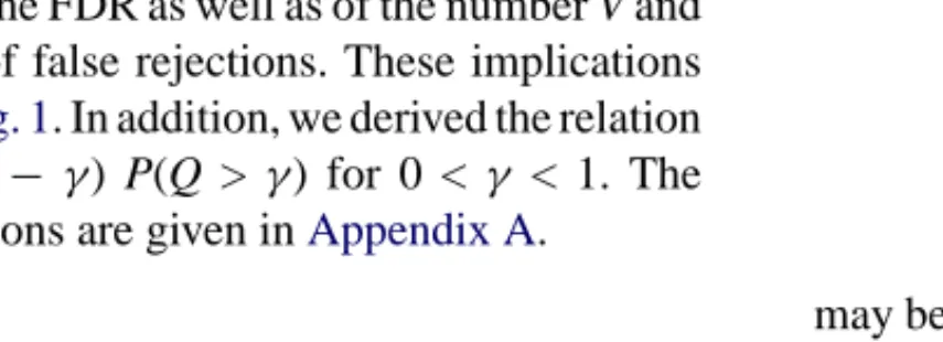
Fig. 1. Relations between control of different type I error rates.
Both, PrAu and PrB␥are based on the permutation prin- ciple and thus are adaptive to the correlation structure of the data.
2.1.4. Relations
The control of the FWE is the most stringent criterion. It implies the control of the FDR as well as of the number V and relative number V/R of false rejections. These implications are demonstrated inFig. 1. In addition, we derived the relation FDR ≤ γ FWE + (1 −γ) P(Q > γ) for 0 < γ < 1. The corresponding derivations are given inAppendix A.
2.2. Simulated data and real data (EEG data) 2.2.1. Simulated data
All procedures considered in this paper can be used for the paired samples case and the case of two independent samples.
They all use the p-values for the different hypotheses. There- fore, it is not necessary to differentiate between the paired samples case and the case of two independent samples. Thus, we only simulated the paired samples case. Let di= xi −yi denote the componentwise differences (i = 1,. . ., k). Thereby in the paired samples case we have the random difference vec- tors d = (d1,. . ., dk) which have k-variate distributions. For these vectors, we generated samples from k-variate normal distributions for special configurations of means and corre- lation coefficients, and executed different multiple tests. The components of k-variate normally distributed vectors d had common variance 1, and the meansµxi−µyi=µdi(i = 1, . . ., k) were chosen so thatµdi =∆(i = 1,. . ., m) andµdi=0 (i = m + 1,. . ., k). This means we considered m false and k− m true hypotheses, and the deviations of the false hypotheses were all into the same direction. The value of m was varied between 1 and k.
We denote the coefficients of correlation between di and dj by ρij (1≤ i ≤j ≤k). We considered the casesρij = 0.2, i.e. constant low positive correlation, andρij = 0.8, i.e.
constant high positive correlation (i=j). In most practical situations, the correlation coefficients ρij do not have the same value and the same sign. Therefore, we also considered the following two types of correlation matrices Corr1 and Corr2. The matrix
Corr1=
1 k−1
k
k−2
k · · · 1 k k−1
k 1 k−1
k · · · 2 k k−2
k
k−1
k 1 · · · 3 k ... ... ... · · · ... 1
k
2 k
3
k · · · 1
may be typical for longitudinal observations, e.g. time series where neighboring observations have higher correlations than more distant observations. The matrix
Corr2=
R1 R2 R2 R2 R1 R2 R2 R2 R1
with
R1=
1 2/3 · · · 2/3 2/3 1 · · · 2/3 ... ... · · · ... 2/3 2/3 · · · 1
and
R2=
−1/3 −1/3 · · · −1/3
−1/3 −1/3 · · · −1/3 ... ... · · · ...
−1/3 −1/3 · · · −1/3
was used in order to investigate a case where both, positive and low negative correlations occur.
The number of repeated simulations for any configuration was 60.000 for most procedures, with the exception of the permutation methods Troe, PrAuand PrB␥where only 5.000 repetitions were done. The number of permutations in each permutation test was 1.000.
2.2.2. EEG data
A sample of 23 female German native speakers partici- pated in the EEG experiment. They auditorily perceived two unrelated wordlists each containing 25 disyllabic abstract nouns. Participants had to memorize the nouns and imme- diately after the presentation of each list they were asked to recall the words previously encoded.
During word encoding EEG was recorded with 19 gold- cup electrodes according to the 10–20 system against the av- eraged signals (A1 + A2)/2 of both ear lobe electrodes. Filter settings were 0.3–35 Hz, sampling frequency was 256 Hz.
According to the behavioral results EEG epochs of subse- quently recalled and not recalled nouns were selected. One second epochs beginning with word onset were Fourier trans- formed and averaged cross-power spectra between all possi- ble electrode pairs (171) were computed for each participant.
As it has been demonstrated, that particularly lower EEG frequencies are associated with dm-effects (differences due to memory performance;Fell et al., 2001; Klimesch et al., 1996;
Weiss and Rappelsberger, 2000), adjacent spectral values were averaged to obtain broad band parameters for the follow- ing frequency bands: delta1 (1–2 Hz), delta (3–4 Hz), theta (5–7 Hz), alpha1 (8–10 Hz), alpha2 (11–12 Hz) and beta1 (13–18 Hz). The normalization of the cross-power spectra yielded 171 coherence values per frequency band, condition (recalled or not recalled) and participant. Coherence values were Fisher-z-transformed for the current statistical analysis.
Further details of the experimental setup and methods of EEG analysis can be found inWeiss and Rappelsberger (2000)and Weiss et al. (2000).
In the present study our aim was to find out which of the 171 pairs of electrodes significantly differ in their means of coherence values for subsequently recalled versus not re- called nouns. For this task we needed a multiple test.
3. Results
3.1. Estimation of the FDR and P(Q > 0.1)
As mentioned inSection 2.1.2, BH and BKY control the FDR under the condition of independence of the test statis- tics or at least of positive regression dependency. In multiple endpoint problems, it is difficult to determine the correlation between the test statistics. However, it may be possible to es- timate the correlation between the endpoints. (Of course, the correlation of the test statistics will be related to the corre- lation of the endpoints.) Thus, we investigated how the FDR of BH and BKY depends on the correlation of the endpoints.
Here the FDR for the correlation structure Corr2 was most in- teresting, as there are negative correlation coefficients.Fig. 2 (left side) demonstrates for Corr2 that the FDR of BH de- creases with increasing m whereas the FDR of BKY does not strongly change when m increases. The FDR of both meth- ods is below the nominal level of 0.05. Similar results were obtained forρ= 0.2,ρ= 0.8 and Corr1.
Fig. 2. Estimates of the FDR and of P(Q > 0.1) for BH (circles) and BKY (triangles) under Corr2 (n = 8, k = 40,α= 0.05,∆= 1.5).
As mentioned inSection 2.1.3, the requirement FDR≤α cannot prevent that V/R attains large values. Therefore, we estimated the probability P(Q > 0.1) for BKY and BH, see Fig. 2(right side). We state that P(Q > 0.1) for BKY and BH is smaller than 0.2.
3.2. Power comparisons
In multiple comparisons, there exist different concepts of power. We will use terms that originally were used in connec- tion with pairwise multiple comparisons. The probability of rejecting at least one of the false hypotheses is called any-pair power, and the probability of rejecting all false hypotheses is called all-pairs power, seeRamsey (1978). If we consider a single false hypothesis, then the probability of rejecting it is called per-pair power, seeEinot and Gabriel (1975).Kwong et al. (2002),Liu (1997) andTroendle (2000)preferred in their power comparisons the average power which is E(R− V)/m, i.e. the expected proportion of false hypotheses that were rejected. In our simulations, we considered equal dif- ferencesµxi−µyi=∆for all m false hypotheses. Then, the per-pair power of each false hypothesis has the same value, say p, so that E(R−V) = mp and with it E(R−V)/m = p. This means that in our considerations the average power is identi- cal with the per-pair power. We restricted our investigations to the per-pair power (average power) and all-pairs power as they seem to be most important in practice.
Our first task was to investigate how the power of our mul- tiple test procedures depends on the fraction m/k of false hy- potheses. We observed that the per-pair power of most method except PrA2increases with increasing m/k, seeFigs. 3 and 4.
However, the all-pairs power curves of most procedures are u-shaped, seeFigs. 5 and 6.
Our second task was to investigate how the power of our methods depends on the correlation structure of the data, see Figs. 3–6. Whenρij =ρfor i=j, i.e. when the correlation is the same for all pairs of components, the per-pair power of BH, BKY and PrA2decreases and that of Troe increases with increasingρ, seeFig. 3, whereas the all-pairs power of all methods increases (only in some cases we state for large m/k a slight power decrease), seeFig. 5.
Fig. 3. Per-pair powers forρ= 0.2 andρ= 0.8 (n = 8, k = 40,α= 0.05,∆= 1.5).
Fig. 4. Per-pair powers under Corr1 and Corr2 (n = 8, k = 40,α= 0.05,∆= 1.5).
Fig. 5. All-pairs powers forρ= 0.2 andρ= 0.8 (n = 8, k = 40,α= 0.05,∆
= 1.5).
Fig. 6. All-pairs powers under Corr1 and Corr2 (n = 8, k = 40,α= 0.05,∆
= 1.5).
Our third task was to investigate how the power of our test procedures depends on the number k of hypotheses. Here the most important result is that the per-pair power of BKY and BH scarcely changes with increasing k, seeFig. 7. The all- pairs power of BKY and BH decreases moderately when the fraction of false hypotheses is small, and slightly when most hypotheses are false, seeFig. 8. As expected, the per-pair power and all-pairs power of the FWE controlling methods Holm and Troe decrease when k increases, seeFigs. 7 and 8.
The powers of Troe, PrAuand PrB␥were not calculated for k
> 40 because of the immense computational effort. We expect that the per-pair power and all-pairs power of PrA2, which are rather high for m/k = 0.2 and k≤40, will decrease very strongly with increasing k, so that they will be much lower for large k than the corresponding power values of BKY and BH.Figs. 7 and 8are forρ = 0.8. The results forρ = 0.2 which are not shown here are very similar.
When we formally compare the different methods we state that PrA2has the highest per-pair power and all-pairs power
Fig. 7. Per-pair powers for m/k = 0.2 and m/k = 0.8 (n = 8,α= 0.05,∆= 1.5,ρ= 0.8).
Fig. 8. All-pairs powers for m/k = 0.2 and m/k = 0.8 (n = 8,α= 0.05,∆= 1.5,ρ= 0.8).
if m/k≤1/4 whereas BKY has the highest per-pair power and all-pairs power if m/k > 1/4. This applies forρ= 0.2 and 0.8 as well as for Corr1 and Corr2, seeFigs. 3–6. However, the per-pair power and all-pairs power of PrA2strongly decrease with increasing k, so that BKY becomes the most powerful method also for small fractions m/k.
3.3. Applications of multiple tests to EEG coherence data
The data we now evaluate come from the experiment de- scribed inSection 2.2.2. The number of subjects was 23. For each subject, a vector of 171 coherence values was obtained under two different conditions. This means we had to test k
= 171 null hypotheses.
In all multiple tests, we used the paired t-test statistics. The number of significant mean differences at levelα= 0.05 with Bonf, Holm and Troe, PrA1and PrA2, PrB0.05, PrB0.1, BL01, BH and BKY are given inTable 2. In the second column are also the number of significant results with the paired t-test which cannot be recommended as it is not a multiple test. Of course, this test provides more significant differences than the multiple tests. Among the multiple tests, most significant differences were found for BKY followed by BH. Among the
Table 2
Number of significant coherence differences for different tests when comparing the processing of subsequently recalled and not recalled nouns for all frequency bands analyzed
t-test FWE≤0.05 P(V > u)≤0.05 P(Q >γ)≤0.05 FDR≤0.05
Bonf Holm Troe PrA1 PrA2 PrB0.05 PrB0.1 BL01 BH BKY
delta1 78 5 6 10 12 25 9 17 7 54 60
delta 64 1 1 7 16 21 7 7 1 44 47
theta 27 4 4 6 7 10 6 6 4 10 10
alpha1 14 0 0 0 1 2 0 0 0 0 0
alpha2 44 0 0 3 7 12 1 1 0 12 12
beta1 55 5 5 5 11 14 7 7 5 23 25
FWE controlling methods, Troe is distinctly more powerful than Bonf and Holm for most frequency bands. It is also more powerful than the FDR controlling procedure BL01 which is considerably less powerful than BKY and BH.
4. Discussion
We have introduced four criteria for controlling type I er- rors (three of them may be new for most readers) and derived the relationships between them, seeFig. 1.
Control of the FWE means to require that no type I error occurs no matter how large the number of hypotheses and the number of rejected hypotheses is. With high-dimensional data, this criterion is too strict. Therefore, the other criteria were proposed.
In our opinion, the requirement P(Q >γ)≤αprovides the most reasonable criterion. Unfortunately, with our program the only corresponding procedure (PrB␥) cannot be executed within an acceptable time of computation when R > 30. In this case, a compromise may be to stop the calculations when R = 30 and report the 30 corresponding (most significant) endpoints. Further research is needed to develop powerful procedures feasible for large k and R.
The requirement P(V > u)≤αis a generalization of the FWE criterion. It is less strict, but it has similar disadvan- tages. In a practical application it is difficult to decide which number u is appropriate. Moreover, the only corresponding procedure (PrAu) requires the same computational effort as PrB␥.
As mentioned in Section 2.1.3, the requirement FDR = E(Q)≤αdoes not prevent that Q attains large values. This is a general disadvantage of the FDR criterion. However,Fig. 2 shows that the probability P(Q > 0.1) is relatively small for the FDR controlling methods BH and BKY. This means that these methods provide a good compromise as they do not strongly violate the requirement of the criterion we favor. Moreover, these two methods are computationally very simple and do not need a special computer program, in contrast to PrAu and PrB␥. In addition, our formal comparisons demonstrated that BKY has a relatively high power. Therefore, this proce- dure seems to be most recommendable. However, caution is needed when comparing methods that satisfy different crite-
ria because one can expect that the strictest criterion leads to the lowest power.
Note that PrAu, PrB␥ and Troe are permutation meth- ods. Such methods have the advantage that they consider the correlation of data. This seems to be the reason why these methods are more powerful forρ= 0.8 than forρ= 0.2, see Figs. 3 and 5.
In order to demonstrate the properties of different multi- ple tests we applied them to EEG coherence data obtained while participants memorized abstract nouns subsequently recalled or not. The major result was that during the phase of word encoding, subsequently recalled nouns elicited higher EEG coherence than not recalled nouns at all electrode pairs showing significant differences. Thus those words which are likely to be recalled are associated with an increase of syn- chronized activity between various brain regions, in particu- lar left hemispheric sites and between both hemispheres. All frequency bands analyzed demonstrated significantly higher coherence for recalled nouns with the exception of the alpha1 band (8–10 Hz), which did not show any significant differ- ences. The latter finding agrees well with the assumption that alpha1 predominantly reflects sensory processing, or gen- eral attentional processes (Klimesch et al., 1996; Weiss and Rappelsberger, 2000), and does not reflect differences in memory encoding. In contrast, coherence in the other fre- quency bands differed considerably for recalled and not re- called abstract nouns. A similar finding to our study was reported byFell et al. (2003)studying intracortical record- ings of the temporal lobe during memory encoding of words.
In addition,Besthorn et al. (1994)found that patients with Alzheimer’s disease, who suffer from a major disturbance of memory functions, exhibited lower coherence than healthy controls in the theta, alpha and beta frequency bands. In our opinion, the higher synchronization for recalled nouns in var- ious frequency bands is associated with the participation of different cognitive operations such as short-time as well as long-time memory, attention to internal thinking, encoding and storage of episodic information and semantic associa- tions occurring during the task, the latter probably being in- creased during the encoding phase and therefore leading to an improved ability to recall the nouns at a later time (Weiss and Rappelsberger, 2000). Multiple tests demonstrate that during the encoding phase subsequently recalled nouns are embedded within a more complicated network of interactions between various recording sites than not recalled nouns.
Acknowledgement
This work was supported by Interdisziplin¨ares Zentrum f¨ur Klinische Forschung Jena, Projekt 1.8, the Austrian Sci- ence Foundation (“Herta Firnberg”-project T127) and the German Science Foundation (SFB 360). We gratefully ac- knowledge the helpful comments of the two referees.
Appendix A
Here are the derivations for the statements given inFig. 1.
We have FDR=E
V R|R >0
P(R >0)
= 0·P V
R =0|R >0
+
w>0
wP V
R =w|R >0
P(R >0)
≤P V
R >0|R >0
P(R >0)
=P(V >0, R >0)=P(V >0)=FWE.
This means FWE≤αimplies FDR≤α. If all hypotheses are true we have V = R. Then FDR= E(V/R|R > 0)P(R > 0) = P(R > 0) = FWE. Thus, in this case FWE and FDR control are equivalent. (If FWE≤αwhen all hypotheses are true then the FWE control is called weak.)
As P(V > u)≤P(V > 0) for u≥0, FWE≤αalso implies P(V > u)≤α.
As P(Q >γ) = P(V >γR)≤ P(V > 0), FWE≤αalso implies P(Q >γ)≤α.
Furthermore, we have FDR= 0·P
V
R =0|R >0
+
0<w≤γ
wP V
R =w|R >0
+
w>γ
wP V
R =w|R >0
P(R >0)
≤ γP
0< V
R ≤γ|R >0
+P V
R > γ|R >0
P(R >0)=B.
Ifγ< 1/k, we have P(0 < V/R≤γ|R > 0) = 0 because V/R cannot take positive values smaller than 1/k. We then obtain B = P(V/R >γ|R > 0)P(R > 0) = P(Q >γ). Thus, P(Q >γ)
≤αimplies FDR≤α, whenγ< 1/k.
If 0 <γ< 1, we have
B= γ
1−P
V
R =0|R >0
−P V
R > γ|R >0
+P V
R > γ|R >0
P(R >0)
=γP(R >0)−γ{P(V =0)−P(R=0)}
+(1−γ)P V
R > γ|R >0
P(R >0)
=γ−γ{1−P(V >0)} +(1−γ)P
V
R > γ|R >0
P(R >0)
=γFWE+(1−γ)P(Q > γ), so that FDR≤γFWE+ (1−γ) P(Q >γ).
References
Benjamini Y, Hochberg Y. Controlling the false discovery rate: a practical and powerful approach to multiple testing. J Roy Stat Soc Ser B 1995;57:289–300.
Benjamini Y, Liu W. A step-down multiple hypotheses testing proce- dure that controls the false discovery rate under independence. J Stat Planning Inference 1999;82:163–70.
Benjamini Y, Liu W. A distribution-free multiple-test procedure that con- trols the false discovery rate. Technical Report. Tel Aviv University, 2001.
Benjamini Y, Yekutieli D. The control of the false discovery rate in multiple testing under dependency. The Ann Stat 2001;29:1165–88.
Benjamini Y, Krieger A, Yekutieli D. Two staged linear step up FDR controlling procedure. Technical Report. Tel Aviv University, 2001.
Besthorn C, Forstl H, Geiger-Kabisch C, Sattel H, Gasser T, Schreiter- Gasser U. EEG coherence in Alzheimer disease. Electroencephalogr Clin Neurophysiol 1994;90:242–5.
Durka PJ, Zygierewicz J, Klekowicz H, Ginter J, Blinowska KJ. On the statistical significance of event-related EEG desynchonization and synchronization in the time–frequency plane. IEEE Trans Biomed Eng 2004;51:1167–75.
Einot I, Gabriel KR. A study of the powers of several methods of multiple comparisons. J Am Stat Assoc 1975;70:574–83.
Fell J, Klaver P, Lehnertz K, Grunwald T, Schaller C, Elger CE, et al. Human memory formation is accompanied by rhinal–hippocampal coupling and decoupling. Nat Neurosci 2001;4:1259–63.
Fell J, Klaver P, Elfadil H, Schaller C, Elger CE, Fern´andez G.
Rhinal-hippocampal theta coherence during declarative memory for- mation: interaction with gamma synchronization? Eur J Neurosci 2003;17:1082–8.
Hemmelmann C, Horn M, Reiterer S, Schack B, S¨usse T, Weiss S. Multi- variate tests for the evaluation of high-dimensional EEG data. J Neu- rosci Methods 2004;139(1):111–20.
Hochberg Y. A sharper Bonferroni procedure for multiple tests of signif- icance. Biometrika 1988;75:800–2.
Hochberg Y, Tamhane AC. Multiple comparison procedures. New York:
Wiley; 1987.
Holm S. A simple sequentially rejective multiple testing procedure. Scand J Stat 1979;6:65–70.
Horn M, Dunnett CW. Power and sample size comparisons of stepwise FWE and FDR controlling test procedures in the normal many-one case. In: Benjamini Y, Sarkar SK, Bretz F, editors. Recent develop- ments in multiple comparison procedures, vol. 47. IMS Lecture Notes Monograph Series; 2004.
Horn M, Hemmelmann C, S¨usse T. A comparative study of test proce- dures for multiple endpoints concerning FDR, FDP FWE and power.
Paper for Meeting of the German MCP Group, Magdeburg, 2003.
Klimesch W, Schimke H, Doppelmayr M, Ripper B, Schwaiger J, Pfurtscheller G. Event-related desynchronisation (ERD) and the Dm effect: does alpha desynchronization during encoding predict later re- call performance? Int J Psychophysiol 1996;24:47–60.
Korn EL, Troendle JF, McShane LM, Simon R. Controlling the number of false discoveries: application to high-dimensional genomic data. J Stat Planning Inference, in press.
Kropf S. Hochdimensionale multivariate Verfahren in der medizinischen Statistik. Aachen: Shaker Verlag; 2000.
Kropf S, L¨auter J, Eszlinger M, Krohn K, Paschke R. Nonparamet- ric multiple test procedures with data-driven order of hypotheses and with weighted hypotheses. J Stat Planning Inference 2004;125:
31–47.
Kwong KS, Holland B, Cheung SH. A modified Benjamini–Hochberg multiple comparisons procedure for controlling the false discovery rate. J Stat Planning Inference 2002;104:351–62.
L¨auter J. Stable multivariate tests for analyzing repeated measurements.
In: Vollmar J, et al., editors. Proceedings of the Eighth DIA Annual European Workshop on Statistical Methodology in Clinical Research and Development, 1997.
Liu W. On step-up tests for comparing several treatments. Stat Sinica 1997;7:957–72.
Ramsey PH. Power differences between pairwise multiple comparisons, comments. J Am Stat Assoc 1978;73:479–87.
Rappelsberger P, Petsche H. Probability mapping: power and coherence analyses of cognitive processes. Brain Topogr 1988;1:46–54.
Sarkar SK. Some probability inequalities for ordered MTP2 random variables: a proof of Simes’ conjecture. Ann Stat 1998;26:494–
502.
Sarkar SK. Some results on false discovery rate in stepwise multiple testing procedures. Ann Stat 2002;30:239–57.
Troendle JF. A stepwise resampling method of multiple testing. J Am Stat Assoc 1995;90:370–8.
Troendle JF. Stepwise normal theory multiple test procedures controlling the false discovery rate. J Stat Planning Inference 2000;84:139–58.
Weiss S, Rappelsberger P. Long-range EEG synchronization during word encoding correlates with successful memory performance. Cogn Brain Res 2000;9:299–312.
Weiss S, M¨uller HM, Rappelsberger P. Theta synchronisation predicts ef- ficient memory encoding of concrete and abstract nouns. NeuroReport 2000;11:2357–61.
Westfall PH, Young SS. Resampling-based multiple testing: Examples and methods for p-value adjustment. New York: Wiley; 1993.
Westfall PH, Tobias RD, Rom D, Wolfinger RD, Hochberg Y. Multiple comparisons and multiple tests using the SAS system. Cary, NC: SAS Institute Inc.; 1999.