Multivariate tests for the evaluation of high-dimensional EEG data
Claudia Hemmelmann
a,∗, Manfred Horn
a, Susanne Reiterer
b,c, Bärbel Schack
a, Thomas Süsse
a, Sabine Weiss
b,daInstitute of Medical Statistics, Computer Sciences and Documentation, University of Jena, D-07740 Jena, Germany
bBrain Research Institute, Cognitive Neuroscience Group, University of Vienna, Vienna, Austria
cNeurological Clinic, University of Tuebingen, Tuebingen, Germany
dSFB 360, University of Bielefeld, Bielefeld, Germany
Received 8 December 2003; received in revised form 20 April 2004; accepted 21 April 2004
Abstract
In this paper several multivariate tests are presented, in particular permutation tests, which can be used in multiple endpoint problems as for example in comparisons of high-dimensional vectors of EEG data. We have investigated the power of these tests using artificial data in simulations and real EEG data. It is obvious that no one multivariate test is uniformly most powerful. The power of the different methods depends in different ways on the correlation between the endpoints, on the number of endpoints for which differences exist and on other factors. Based on our findings, we have derived rules of thumb regarding under which configurations a particular test should be used. In order to demonstrate the properties of different multivariate tests we applied them to EEG coherence data. As an example for the paired samples case, we compared the 171-dimensional coherence vectors observed for the alpha1-band while processing either concrete or abstract nouns and obtained significant global differences for some sections of time. As an example for the unpaired samples case, we compared the coherence vectors observed for language students and non-language students who processed an English text and found a significant global difference.
© 2004 Elsevier B.V. All rights reserved.
Keywords: Coherence; EEG data; Global hypothesis; Language; Multiple endpoints; Multivariate test; Permutation test; Power of test
1. Introduction
The improvement of EEG/MEG measurement equipment permits the registration of a high number of channels. Ad- ditionally, modern analysis procedures yield large sets of high-dimensional parameters, which have to be evaluated statistically. Furthermore, the statistical evaluation of spec- tral parameters of different frequency bands becomes nearly unmanageable.
Many authors use an α-level test for each single com- ponent or endpoint of the observational vector, see e.g.
Rappelsberger and Petsche (1988). However, this practice results in a large number of false positive statements. There exist several techniques to cope with this general drawback in multiple comparisons. Corresponding multiple tests will be considered in a forthcoming paper. In this paper, we will deal with so-called global tests or multivariate tests. A
∗Corresponding author. Tel.:+49-3641-9-33610;
fax:+49-3641-9-33200.
E-mail address: hemmel@imsid.uni-jena.de (C. Hemmelmann).
multivariate test provides one joint statement on all end- points, whereas a multiple test provides a statement for each endpoint.
A well-known multivariate test is Hotelling’s T2-test.
However, this test cannot be executed if the dimension of the data is higher than the number of subjects, which is the usual situation in EEG studies. Another drawback is that the T2-test requires multivariate normal distribu- tions. Therefore, several new statistical methodologies have been developed. Recently, several authors have proposed special test statistics in permutation tests for evaluating high-dimensional EEG data (see e.g.Karniski et al., 1994;
Galan et al., 1997; Harmony et al., 2001). Permutation tests do not require special distributions and have several other advantages (seeLudbrook and Dudley, 1998).
Our paper has the following aims: (a) to give an overview of appropriate multivariate tests including novel methods, (b) to study and to compare the power characteristic of dif- ferent multivariate tests using simulations with different data configurations, (c) to derive general rules for determining which test is suitable for which configuration, and (d) to
0165-0270/$ – see front matter © 2004 Elsevier B.V. All rights reserved.
doi:10.1016/j.jneumeth.2004.04.013
demonstrate the use of different multivariate tests in compar- isons of large sets of coherence values obtained from EEG recordings during language processing in one group of sub- jects under different conditions (paired samples problem) and in two groups of subjects performing the same cognitive task (two independent samples problem).
2. Methods
2.1. Multivariate tests
In analogy to the univariate case, we must differentiate between the case of paired samples and unpaired samples, i.e. two independent samples. In the paired samples case, we observe n subjects under two different conditions, say A and B. In the case of two independent samples, we observe n1 subjects under condition A and n2subjects under condition B.
Our observations are vectors of dimension k. Let x = (x1, . . . , xk)and y=(y1, . . . , yk)denote the random vec- tors with means(µx1, . . . , µxk)and(µy1, . . . , µyk), respec- tively. In the paired and the unpaired samples case, x stands for the observations under condition A and y under condi- tion B. We now can formulate the individual null hypothe- ses H1 : µx1 = µy1, . . . , Hk : µxk =µyk and the global hypothesisH0 : µx1 = µy1, . . . , µxk =µyk. This means, H0is the intersectionH0=H1∩. . .∩Hk. Tests for H0are called global tests or multivariate tests, tests forH1, . . . , Hk
are called multiple tests.
2.1.1. The methods of Bonferroni and Simes
The simplest way to test H0 at levelαis to test all in- dividual hypothesesH1, . . . , Hk at level α/k and to reject H0, if and only if, at least one Hi can be rejected. This is the well-known Bonferroni method. LetP1, . . . , Pk be the P-values obtained when testingH1, . . . , Hk, and letP(1)≤ . . . ≤ P(k) denote the ordered Pi. Then, the Bonferroni method rejects H0ifP(1)≤α/k.
Another simple test is the global test of Simes (1986).
This test rejects H0ifP(i)≤αi/kfor at least one i (1≤i≤ k). Note, that the mathematical proof that this test keeps the α-level was given only for the case of uncorrelated P-values.
However, simulations bySimes (1986),Samuel-Chan (1996) and other authors permit the conclusion that with two-sided comparisons theα-level is always kept. It is also kept with one-sided comparisons when the P-values are positively correlated. Only with negative correlations a slight but ac- ceptable anti-conservativeness could be observed. Hence, there are no practical objections against using this test, generally.
A disadvantage of the Bonferroni method and the Simes test is that they cannot take into consideration the correlation between the endpoints or P-values. Nevertheless, with cer- tain configurations they have higher power than some other tests that consider the correlation, seeSection 3.
2.1.2. Methods of the O’Brien type
A pure multivariate test, which considers the correlation, is Hotelling’s T2-test, which is well known. However, as al- ready mentioned in Section 1, this test is not appropriate for the analysis of EEG data, which comprise many com- ponents with few subjects. Another disadvantage is that this test requires k-variate normal distributions. The T2-test has also the drawback that it cannot differentiate between any departures from H0and departures of all endpoints into the same direction, i.e. it is not very sensitive against effects in the same direction.
In order to overcome the latter disadvantage of the T2-test, several attempts have been made, e.g. in O’Brien (1984), Pocock et al. (1987),Tang et al. (1989). The rationale behind all methods proposed is the following: For each subject, one calculates a single score from its k component values. In this way, the k-variate problem is reduced to a univariate prob- lem. With these scores, the matched pairs t-test is executed in the paired samples situation and the two-sample t-test in the two independent samples situation. For example, the score belonging to a subject of the so-called ordinary least squares (OLS) test of O’Brien is simply the sum of its standardized component values, and OLR stands for a version that uses the corresponding ranks. Unfortunately, it turned out that with these methods theα-level could not be kept when the sample sizes are small, i.e. these tests are anti-conservative, see Kropf (2000), Reitmeir and Wassmer (1996), Frick (1997). However, Läuter et al. (1996) succeeded in con- structing corresponding tests that exactly keep the α-level that are sensitive against departures from H0 either in one direction or in both directions, and that can be used with any k and n. We will consider three different tests ofLäuter et al. (1996), namely the standardized sum test (SS test), the principal component test (PC test) without scale correction and the PC test with scale correction. The SS test is sensitive against departures from H0 in all endpoints into the same direction. With this test, the different components may be measured in different scales, e.g. one in mm, another in kg, etc. or also if the ranges of possible values are different, e.g.
if the range of one endpoint is 1–10 mm and the range of an- other endpoint 20–50 mm. The PC test with scale correction should be used if the different endpoints are measured in dif- ferent scales or if the endpoints differ in their ranges. Other- wise, the PC test without scale correction is recommended.
Useful descriptions of Läuter tests and other tests of the O’Brien type can be found inBregenzer (2000)as well as in Kropf (2000).
These tests have one of the disadvantages of the T2-test:
they require k-variate normality. Tests that do not require special distributions are permutation tests.
2.1.3. Permutation tests
The idea of permutation tests is an old one, however their broad practical application became possible only by fast computers. Below we will use numerical examples in order to explain the permutation principle for paired
Table 1
Permutations of paired samples data of dimensionk=2 withn=3 subjects, and values of different test statistics
Permutation Subject (x1, x2) (y1, y2) t1 t2 tsum t|sum| tmax
1 (original data) 1 (8, 6) (5, 2) 3.46 5.20 8.66 8.66 5.20
2 (4, 3) (3, 1)
3 (6, 7) (4, 4)
2 1 (8, 6) (5, 2) 0.46 0.48 0.94 0.94 0.48
2 (4, 3) (3, 1)
3 (4, 4) (6, 7)
3 1 (8, 6) (5, 2) 1.11 0.90 2.01 2.01 1.11
2 (3, 1) (4, 3)
3 (6, 7) (4, 4)
4 1 (8, 6) (5, 2) 0.00 −0.15 −0.15 0.15 −0.15
2 (3, 1) (4, 3)
3 (4, 4) (6, 7)
5 1 (5, 2) (8, 6) 0.00 0.15 0.15 0.15 0.15
2 (4, 3) (3, 1)
3 (6, 7) (4, 4)
6 1 (5, 2) (8, 6) −1.11 −0.90 −2.01 2.01 −1.11
2 (4, 3) (3, 1)
3 (4, 4) (6, 7)
7 1 (5, 2) (8, 6) −0.46 −0.48 −0.94 0.94 −0.48
2 (3, 1) (4, 3)
3 (6, 7) (4, 4)
8 1 (5, 2) (8, 6) −3.46 −5.20 −8.66 8.66 −5.20
2 (3, 1) (4, 3)
3 (4, 4) (6, 7)
sample and two independent sample analyses that employ t-statistics.
2.1.3.1. Paired samples. We consider an artificial numeri- cal example given inBlair and Karniski (1993), seeTable 1.
The sample size is n = 3, the dimension of observational vectors x and y isk=2.
The total number of permutations is 2n=23=8. What we call permutation 1 is the original data. A permutation is obtained by exchanging the x-vector of a subject for the y-vector of the same subject. Note that complete x- and y-vectors must be exchanged as their components are corre- lated. In this way, permutation 2 was obtained by exchang- ing the x-vector for the y-vector of subject 3, permutation 3 by exchanging the x-vector for the y-vector of subject 2, permutation 4 by exchanging the x-vectors for the y-vectors of subjects 2 and 3, etc. This approach is justified because all such permutations are equally likely when the null hy- pothesis of no difference between the two conditions is true.
Now, for each permutation, the paired samples t-statistic was calculated separately for each component. t1 is the t-value when comparing x1and y1, and t2when comparing x2and y2. In order to combine the information from the uni- variate test statistics in a single multivariate test statistic, we have various possibilities. We can calculatetsum =k
j=1tj
ort|sum|=k
j=1|tj|ortmax=tj, wheretj is equal to the tj (j =1, . . . , k) which has the greatest absolute value. These
test statistics were already used inBlair et al. (1994). In our example we have tsum = t1+t2, t|sum| = |t1| + |t2| and tmax=t1if|t1|>|t2|ortmax=t2if|t1| ≤ |t2|.
The different test statistics are sensitive to different spe- cific forms of departures from H0. tsumis sensitive to depar- tures of all endpoints in the same direction, in contrast to t|sum|. tmaxis sensitive to departures in only a few endpoints.
Other appropriate multivariate test statistics are the t-values of the Läuter tests which are denoted by tSSfor the SS test and by tPC for the PC test without scale correction and by tPC+for the PC test with scale correction. The use of these test statistics in permutation tests was already proposed in Kropf (2000).
The statistic t|sum|permits only two-sided testing, in con- trast to the other statistics. One-sided testing requires to specify a direction of testing in advance. In our example, one-sided testing means to show that the mean vector of x1 and x2tends to be greater than that of y1and y2. Two sided testing does not specify a direction.
The sampling distribution of multivariate permutation statistics is obtained by computing the desired test statis- tic for all permutations. As under H0 all permutations are equally likely, we can easily calculate the P-value, i.e. the probability of obtaining an observation which under H0 is at least as extreme as that of the original data. In our case, the P-value is the number of permutations for which the test statistic has a value not smaller than that of the original
data, divided by the total number of permutations. In our example, the test statistics tsum, t|sum|, and tmax attain their maximum value for permutation 1, i.e. for the original data.
Therefore, the probability of obtaining for tsum a value not smaller than 8.66 is 1/8 = 0.125 as only one of the eight tsumvalues is not smaller than 8.66, i.e. the one-sided P-value is 0.125. The same applies to tmax. For t|sum| we have only a two-sided test. Its P-value is 2/8 = 0.25. In order to calculate two-sided P-value for tsum (or tmax), we determine the number of permutations where the absolute value of tsum (tmax) is equal to or greater than the corre- sponding absolute value for the original data, and divide it by the number of permutations. Then the two-sided P-value for tsum(and tmax) is 0.25.
If n is large, it is difficult to perform the calculations for all 2n permutations. Then, the so-called Monte Carlo method is used which means that M permutations are randomly se- lected out of all possible permutations. The P-value is then the number of permutations for which the test statistic has a value not smaller than that for the original data, divided by M. The difference between the exact and the Monte Carlo method is negligible when M is large.
2.1.3.2. Two independent samples. Before we explain the permutation test for two independent samples we introduce a new multivariate test statistics for two-sided comparisons of two independent samples. Its use in permutation tests showed a surprisingly high power for some configurations, seeSection 3. The suggestion comes fromGood (2000)who used the termn2
i=1(yi− ¯x)2in a test statistic for detecting differences between means in the univariate case for a special situation.
Let the k-variate observations we obtain for two indepen- dent samples be given in a data matrix
x11 · · · x1k
... ...
xn11 · · · xn1k
y11 · · · y1k
... ...
yn21 · · · yn2k
.
For all components, we calculate the sample means
¯
xj = (1/n1)n1
i=1xij and y¯j = (1/n2)n2
i=1yij, the sample variances s2xj = (1/(n1 − 1))n1
i=1(xij − ¯xj)2 and s2yj = (1/(n2 − 1))n2
i=1(yij − ¯yj)2, and the dif- ferences vij = (yij − ¯xj)/
sy2j+s2xj/n1 and wij = (xij − ¯yj)/
sx2j+s2yj/n2 (j = 1, . . . , k). Note that the denominators in vij and wij are the estimates of the stan- dard deviations of the respective numerators. Now we calculate the means v¯ = (1/kn2)k
j=1
n2
i=1vij and w¯ = (1/kn1)k
j=1
n1
i=1wij, the differencesaij = vij− ¯v (i =
1, . . . , n2,j =1, . . . , k) anda∗ij=wij− ¯w(i=1, . . . , n1, j =1, . . . , k), and the component-wise test statisticsaj = (1/n2)n2
i=1a2ij+(1/n1)n1
i=1(a∗ij)2(j=1, . . . , k). Finally we determine ta = max{a1, . . . , ak}, which is the new global test statistic we propose. Note that aj(j=1, . . . , k) and with it taare symmetric in x and y, i.e. exchanging the two samples gives the same value.
The rationale behind this proposal will be explained under simplifying assumptions. Let the mean vectors(µx1, ..., µxk) and(µy1, ..., µyk)differ in exactly m components, for ex- ampleµyi−µxi =∆i (i=1, . . . , m) andµyi−µxi =0 (i=m+1, . . . , k). Assume that n1and n2are very large, so thats2xjands2yjcan be replaced by their respective expec- tationsσx2j andσy2j, ands2xj/n1ands2yj/n2by 0. In addition assume thatσ2xj =σy2j=σj2. Then
E(aij)=E(yij)−E(x¯j)
σj −E(¯v)= ∆j σj −1
k
m l=1
∆l σl, and
E(a∗ij) =E(xij)−E(y¯j)
σj −E(w)¯ = − ∆j
σj −1 k
m l=1
∆l
σl
(j=1, . . . , m).
Thus, for large values of |∆j/σj| we can expect that|aij|and
|a∗ij|with it aj and finally taare large.
Note thatE(aij) =E(a∗ij)=0, ifm =k and∆1/σ1 =
· · · =∆k/σ, so that ta provides a low power. This can be seen in our simulation results inFigs. 3 and 4inSection 3.
However, such a situation will rarely be met in practice.
We now explain the permutation principle when com- paring two independent samples. Again, we use a simple numerical example, seeTable 2. The two independent sam- ples have the sizesn1=3 (subjects under condition A) and n2=2 (subjects under condition B). The dimension of the observational vectors x and y isk=2. Permutation 1 is the original data. The way of permuting is different from that in the paired samples case. We now exchange vectors observed in subjects under A for vectors observed in (other) subjects under B. So permutation 2 was obtained by exchanging the x-vector of the first subject of the sample under A for the y-vector of the first subject of the sample under B, permu- tation 3 by exchanging the x-vector of the second subject under A for the y-vector of the first subject under B, etc. In this way we obtain(n1+n2)!/(n1!n2!)=5!/(3!2!)=10 permutations. The justification for this approach is similar as in the paired samples case. Now, for each permutation, the values t1 and t2 of the t-statistic for the case of two independent samples were calculated separately for each of the two components. Finally, the multivariate test statistics tsum, t|sum|, and tmax were calculated from t1 and t2 in the same way as in the paired samples case. In addition, the new test statistic ta was calculated. Now, the P-values can be calculated as described for the paired samples case. For
Table 2
Permutations of two-dimensional data of two independent samples with sizesn1=3 andn2=2, and values of different test statistics
Permutation (x1, x2) (y1, y2) t1 t2 tsum t|sum| tmax ta
1 (original data) (8, 6) (5, 2) 1.20 2.40 3.60 3.60 2.40 1.72
(4, 3) (3, 1)
(6, 7)
2 (5, 2) (8, 6) −0.25 0.18 −0.07 0.43 −0.25 0.82
(4, 3) (3, 1)
(6, 7)
3 (8, 6) (4, 3) 2.37 1.42 3.79 3.79 2.37 1.22
(5, 2) (3, 1)
(6, 7)
4 (8, 6) (6, 7) 0.61 −0.12 0.59 0.73 0.61 0.97
(4, 3) (3, 1)
(5, 2)
5 (3, 1) (5, 2) −1.36 −0.12 −1.48 1.48 −1.36 1.22
(4, 3) (8, 6)
(6, 7)
6 (8, 6) (5, 2) 0.61 0.89 1.50 1.50 0.89 0.78
(3, 1) (4, 3)
(6, 7)
7 (8, 6) (5, 2) −0.25 −0.44 −0.69 0.69 −0.44 0.77
(4, 3) (6, 7)
(3, 1)
8 (5, 2) (8, 6) −0.71 −0.44 −1.15 1.15 −0.71 0.84
(3, 1) (4, 3)
(6, 7)
9 (5, 2) (8, 6) −2.85 −5.40 −8.25 8.25 −5.40 3.94
(4, 3) (6, 7)
(3, 1)
10 (8, 6) (4, 3) 0.17 −0.81 −0.64 0.98 −0.81 1.10
(5, 2) (6, 7)
(3, 1)
example, as we have two permutations with tsum ≥ 3.60, the one-sided P-value for tsumis 2/10=0.2. The one-sided P-value for tmaxis 0.1. The two-sided P-values for tmaxand taare 0.2, and for tsum and t|sum| are 0.3.
2.2. Artificial data and real data (EEG data) 2.2.1. Artificial data
We generated samples from k-variate normal, exponen- tial and log-normal distributions for special configurations of means and correlation coefficients, and executed the dif- ferent multivariate tests described inSection 2.1. The com- ponents of k-variate normally distributed vectors x and y had common variance 1. For all distributions, the means µx1, ..., µxkandµy1, ..., µykwere chosen so, thatµyi−µxi =
∆(i=1, . . . , m) andµyi−µxi =0 (i=m+1, . . . , k).
This means we considered m false and k−m true hypotheses, and the deviations of the false hypotheses were all into the same direction. The value of m was varied between 1 and k.
In the paired samples case, we denote the coefficients of correlation between the differencesxi−yiandxj−yjbyρij (1 ≤ i≤j ≤k). In the case of two independent samples,
ρij denotes the coefficient of correlation between the com- ponents xiand xjas well as between the components yiand yj (1≤i≤j ≤k). For both paired and unpaired samples, we first considered the case ρij =ρ (i = j), i.e. constant (low, moderate or high) correlation. However, in most prac- tical situations, the correlation coefficientsρij do not have the same value and the same sign. Therefore, we also consid- ered the following two types of correlation matrices Corr1 and Corr2. The matrix
Corr1=
1 k−1
k
k−2
k · · · 1 k−1 k
k 1 k−1
k · · · 2 k−2 k
k
k−1
k 1 · · · 3 ... ... ... · · · k...
1 k
2 k
3
k · · · 1
may be typical for longitudinal observations, e.g. time se- ries where neighboring observations have higher correlations
than more distant observations. The matrix
Corr2=
R1 R2 R2 R2 R1 R2 R2 R2 R1
with
R1=
1 2/3 · · · 2/3 2/3 1 · · · 2/3 ... ... · · · ...
2/3 2/3 · · · 1
and
R2=
−1/3 −1/3 · · · −1/3
−1/3 −1/3 · · · −1/3 ... ... · · · ...
−1/3 −1/3 · · · −1/3
was used in order to investigate a case where both, positive and negative correlations occur.
The number of repeated simulations for any configuration was 5000, the number of permutations in each permutation test was 1000.
2.2.2. EEG data
The EEG was recorded with 19 gold-disc electrodes ac- cording to the 10–20 system against the averaged signals (A1+A2)/2 of both ear lobe electrodes. Filter settings were 0.3–35 Hz, sampling frequency was 256 Hz. Epochs with ar- tifacts were eliminated from further processing.
2.2.2.1. Word processing under different conditions.
Twenty-three right-handed female native German speakers participated in the experiment (age 22–26). Two word lists each containing either 25 concrete or 25 abstract German nouns were selected and psycholinguistically controlled (e.g. Weiss and Müller, 2003). Nouns had a mean word length of 0.9 s±0.08 and were auditorily presented with an interstimulus interval of 2.5 s. Participants were requested to memorize the presented nouns and had to recall them af- ter the presentation. A trigger marked the beginning of each word presentation, and the following 1 s EEG epochs were selected for coherence analysis. Instantaneous coherence values for each electrode pair of the alpha1-band (8–10 Hz) were computed with a time resolution of approximately 4 ms in accordance with the sampling frequency of 256 Hz on the basis of an ARMA model with time-varying model parameters (see e.g.Schack et al., 1999, 2003). The chosen frequency resolution was 0.5 Hz. Averaging was performed within the alpha1-band (8–10 Hz) over adjacent spectral lines. For each trial 250 instantaneous coherence values were obtained. The next step was averaging over the single trials time point by time point. For data reduction, the 1 s trials were divided into 10 sections of 100 ms. This yielded
10 coherence values per presentation mode and per word category.
The comparison of coherence values for all 171 electrode pairs accompanying concrete and abstract nouns processing requires a multivariate test for paired samples.
2.2.2.2. Foreign language processing by different groups.
A group of 19 foreign language students (all studying En- glish language and linguistics at university level) and a sec- ond group of 19 non-language students (studying other sub- jects than languages), all mother-tongue German speakers, participated in the experiment. The subjects had to watch various video sequences of TV news on a TV screen. The stimulus material used in this study comprised nine individ- ual tasks. Each task was a sequence of an approximately 2 min video-recorded TV news text. The TV news texts were presented in British English, in American English and in Austrian German, and in three modalities: visual+auditory (TV mode), auditory only and visual only. Looking at a gray flickering picture was chosen as a control situation in order to control individual base-line effects.
For all electrode pairs ordinary coherence values of the alpha1-frequency band (8–10 Hz) were calculated according to the Bartlett algorithm by using 2 s intervals for averaging procedures.
We evaluated one of the three TV-news (British English) which were presented in TV mode (visually +auditory).
The comparison of the 171-dimensional vectors of coher- ence values of the two groups of subjects requires a multi- variate test for two independent samples.
3. Results
3.1. Power characteristics and power comparisons Power is a statistical term. The power of a multivariate test is the probability of rejecting the global null hypothesis if it is false. It may depend on various quantities, e.g. the corre- lation between the components, the number of components, the number of components where differences exist, etc. In order to estimate the power and to study its dependence on these quantities it is common to perform computer simula- tions. For this purpose, we generated samples from k-variate distributions as described inSection 2.2.1, and applied the different multivariate tests introduced inSection 2.1. The re- sults reported in the sequel are restricted to two-sided testing and to normal distributions. The results for other distribu- tions were similar. They are not shown here.
We observed that the power of most (but not all) meth- ods increases with increasing m/k. This is what one would expect.
When ρij = ρ for i = j, i.e. when the correlation is the same for all pairs of components, the influence of the correlation on the power is different for different methods, seeFigs. 1 and 2.
Fig. 1. Power dependence on the correlationρin the paired samples case form=5 (left side) andm=35 (right side) (k=40,n=20,∆=0.4, α=0.05).
The power of the permutation test with tmaxis higher than the power of all other methods, if m/k is small, seeFig. 1, left side. A comparison of the remaining methods shows that the Simes method and the Bonferroni method have a relatively high power if ρ is small or medium. A different characteristic and rank order of the methods can be observed if m/k is large, seeFig. 1, right side. Note also that with large m/k the power decreases when ρ increases. This tendency was also reported in other papers, e.g. inBlair et al. (1994).
tmaxis superior also with medium m/k as long as the cor- relation is high, see Fig. 2, right side. However, tmax and also Bonferroni and Simes are inferior with low correlation and large m/k, seeFig. 2, left side. Note that in each situa- tion a better test exists than the methods of Simes or Bon- ferroni. This applies also for the two independent samples case. Hence, in the power plots for this case we will omit the Simes and Bonferroni methods.
In the two independent samples case, we obtained similar results as in the paired samples case when using the same
Fig. 2. Power dependence on m/k in the paired samples case forρ=0.2 (left side) andρ=0.8 (right side) (k=40,n=20,∆=0.4,α=0.05).
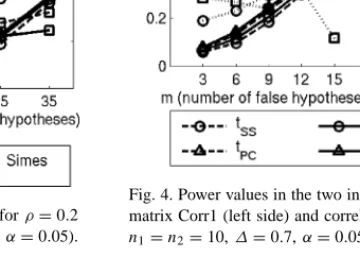
Fig. 3. Power values in the two independent samples case fork=20 (left side) andk=100 (right side) (ρ=0.8,n1=n2 =10,∆=0.7, α=0.05).
test statistics. When applying the new statistic taintroduced inSection 2.1.3.2, we obtained more powerful tests for equal correlations, seeFig. 3. Note that the power of the test with ta is higher for k =100 than fork = 20 when m/k is 0.1 or 0.9, whereas the power of the other tests seems to be independent of k. Only, when m = k, ta provides a low power, see alsoFig. 4. The explanation is given inSection 2.1.3.2.
When considering the correlation structures given by the matrices Corr1 and Corr2, we obtained the power estimates in Fig. 4. Under Corr1 the power curves do not differ so strongly as under Corr2 where the tests with tSS and tsum are distinctly better. Under both correlation structures tapro- vides low power. However, as already mentioned, in these simulations all m mean differencesµyi−µxiwere positive.
If we considered positive and negative differences, the power for tSSand tsumwould be lower and the power for tahigher.
Table 3provides an overview of which methods were best in which configuration. The statements there may be helpful
Fig. 4. Power values in the two independent samples case with correlation matrix Corr1 (left side) and correlation matrix Corr2 (right side) (k=15, n1=n2=10,∆=0.7,α=0.05).
Table 3
Best multivariate tests under different configurations for paired samples and two independent samples
Correlation Relative number of false hypotheses Paired samples Two independent samples
ρ=0.2 Small tmax, Simes, Bonferroni ta
Medium t|sum| t|sum|
Large t|sum|, tsum, tSS, tPC t|sum|, OLS, tSS
ρ=0.8 Small tmax ta
Medium tmax ta
Large tmax, t|sum|, tsum tSS, t|sum|
Corr1 Small tmax ta
Medium tmax tmax
Large tsum, t|sum|, tSS, tPC tsum, t|sum|, tSS, tPC
Corr2 Small tsum, tSS tsum, OLS, tSS, OLR
Medium tsum, tSS tsum, OLS, tSS, OLR
Large tsum, tSS, t|sum| tsum, OLS, tSS, OLR
to decide which of the different tests or test statistics should be used for evaluating data at hand.
3.2. Applications of multivariate tests to EEG coherence data
3.2.1. Paired samples of word processing under two different conditions
The data we now evaluate come from the experiment described inSection 2.2.2.1. The number of subjects was 23. For each subject, a vector of 171 coherence values was obtained under two different conditions, namely under the processing of either concrete or abstract nouns. The co- herence values are given for 10 sections of time: 0–100, 100–200, . . ., 900–1000 ms. For each section, we tested the global hypothesis of no difference between concrete and abstract nouns processing in all 171 components. The P-values obtained for the permutation test with the differ- ent test statistics are given inTable 4. P-values smaller than 0.05 are in bold type, which means that the correspond- ing tests rejected the global hypothesis at the 5% level.
The P-values for the Bonferroni and the Simes methods are omitted. Neither rejected the global hypothesis. The pure Läuter tests also did not provide significance in contrast to permutation tests that used the Läuter test statistics. It can
Table 4
P-values of the multivariate permutation test with different test statistics for 10 sections of time Test Time in ms
0–100 100–200 200–300 300–400 400–500 500–600 600–700 700–800 800–900 900–1000
tsum 0.0164 0.1202 0.1216 0.3455 0.0344 0.0482 0.3091 0.3433 0.6591 0.5607
t|sum| 0.0212 0.1462 0.0842 0.1910 0.0230 0.0308 0.2198 0.2743 0.4269 0.5005
tmax 0.2845 0.0368 0.0660 0.0576 0.0252 0.0174 0.0458 0.0336 0.2517 0.7197
tSS 0.0144 0.1218 0.1290 0.3575 0.0336 0.0526 0.3133 0.3477 0.6591 0.5581
tPC 0.0138 0.0928 0.0640 0.1616 0.0202 0.0208 0.2250 0.2887 0.5581 0.5167
tPC+ 0.0148 0.1022 0.0732 0.2216 0.0236 0.0308 0.2835 0.3285 0.5617 0.5143
be seen that in different sections different tests provided significance.
3.2.2. Paired samples from longitudinal observations of word processing for only one component under two different conditions
In this section, we consider the same data as in the for- mer section. However, we now evaluate only the coherence values obtained for one of the 171 components, namely for the electrode pair P3/O1, as a function of time. As we have 10 sections of time, we have a multivariate test problem of dimension k=10. The mean coherence values under pro- cessing of abstract and concrete nouns are given for the 10 sections of time inFig. 5, left side.
This illustration and also the boxplots of the pairwise dif- ferences inFig. 5, right side, suggest that the presentation of abstract nouns results in higher coherence values than the presentation of concrete nouns for this electrode pair.
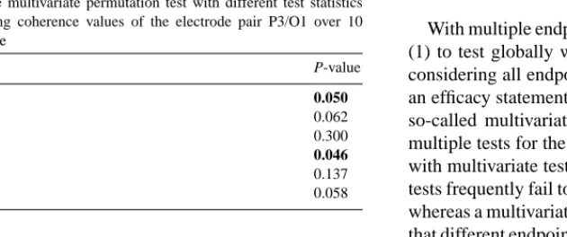
When we separately test each of the 10 differences with the Wilcoxon test, we obtain P-values greater than 0.05, see Fig. 5, right side. However, the P-values of the multi- variate permutation tests with the test statistics tsumand tSS
are 0.05 and 0.046, respectively, seeTable 5. This permits the rejection of the global null hypothesis and confirms that the curve of coherence values over the 10 sections of time
Fig. 5. Mean coherence values for the electrodes P3 and O1 for abstract and concrete nouns processing (left side) and corresponding boxplots and Wilcoxon test P-values of coherence differences (right side).
Table 5
P-values of the multivariate permutation test with different test statistics when comparing coherence values of the electrode pair P3/O1 over 10 sections of time
Test statistics P-value
tsum 0.050
t|sum| 0.062
tmax 0.300
tSS 0.046
tPC 0.137
tPC+ 0.058
is significantly higher for abstract nouns than for concrete nouns.
3.2.3. Independent samples data of foreign language processing by two different groups
In this section, we evaluate data of the experiment as de- scribed inSection 2.2.2.2. The aim is to compare coherence values of the language students and the non-language stu- dents. Again, for each student a vector of 171 coherence val- ues is given. We have to test the global null hypothesis that the vectors of both groups have the same expectations. The P-values of the permutation test with different test statis- tics are given in Table 6. At the 5% level, we can reject the global null hypothesis of no difference between the two groups with the test statistics tsum, t|sum|, tmax, tSS, and ta.
Table 6
P-values for the multivariate permutation test with different test statistics when comparing coherence values of language and non-language students
Test statistics P-value
tsum 0.037
t|sum| 0.049
tmax 0.026
tSS 0.035
tPC 0.072
tPC+ 0.052
ta 0.048
4. Discussion
With multiple endpoints, two different aims are of interest:
(1) to test globally whether there is an overall effect when considering all endpoints simultaneously and (2) to provide an efficacy statement for each individual endpoint. We need so-called multivariate or global tests for the first aim and multiple tests for the second aim. In this paper we only deal with multivariate tests. It should be mentioned that multiple tests frequently fail to detect effects for individual endpoints, whereas a multivariate test provides significance. This means that different endpoints may jointly explain a treatment effect when using a multivariate test.
In this paper, we have introduced several multivariate tests with an emphasis on multivariate permutation tests. The computational effort of permutation tests is relatively high.
But permutation tests have various advantages.Good (2000) states: ‘Permutation tests permit us to choose the test statis- tic best suited to the task at hand’.
All simulation results presented in this paper were ob- tained under k-variate normality. With exponential and log-normal distributions we obtained similar results as with normal distributions. Hence, they are not reported in this paper.
Our investigations of the varying power characteristics showed that among the different multivariate tests or test statistics, no specific one can be determined as the best.
It depends, on the correlation structure, on the number of endpoints for which differences exist, on the magnitude of the differences, on the total number of endpoints and on other factors, which test is able to reject the global hypothesis.
Thus, prior knowledge concerning the correlation between the components and the relative number of components at which differences exist should be used to find an appropriate multivariate test. Advice and recommendations as to which methods are appropriate can be found inTable 3ofSection 3.1.
In order to demonstrate the properties of different mul- tivariate tests we applied them to EEG coherence data
obtained while participants processed either different word categories or an English text.
Firstly, multivariate tests for paired samples were applied to the processing of concrete and abstract nouns. It is well known that processing of concrete and abstract nouns dif- fers in various ways, which has been assessed with several different neuro-physiological and -psychological techniques (e.g.Bleasdale, 1987; Coltheart, 1987; Kiehl et al., 1999;
Weiss et al., 1999). With several of our tests, we obtained significant global differences between the 171-dimensional coherence vectors for concrete and abstract nouns for the time intervals between 0–200 and 400–800 ms. These find- ings partly correspond to previous results on phase relations which showed the most prominent differences between con- crete and abstract nouns processing between 300–500 and 600–800 ms, respectively (Schack et al., 2003). The time intervals showing the most significant differences coincide with the results of an ERP-study of West and Holcomb (2000), who noticed that concrete words elicited a more neg- ative ERP than abstract words between 300 and 800 ms.
Secondly, multivariate tests for independent samples were applied to EEG coherence data from high and low proficiency second language speakers processing English TV news reports. It is a commonsense argument that people differ in their proficiency and amount of training in their second languages, hence have different levels of perfor- mance. EEG coherence has been used to detect the differ- ences between high and low foreign language performers (Reiterer and Rappelsberger, 2001). A significant global difference between the 171-dimensional vectors of coher- ence values (intensity of coherence) of language students and non-language students could be found with most of our multivariate tests. Obviously, this was caused by differences for most electrode pairs with a tendency of larger coherence values for language students.
Acknowledgements
We would like to thank the two referees for their use- ful comments and suggestions. This work was supported by Interdisziplinäres Zentrum für Klinische Forschung Jena, Projekt 1.8, by the Austrian Science Foundation (“Herta Firnberg”—project T127) and the German Science Founda- tion (SFB 360).
References
Blair RC, Karniski W. An alternative method for significance testing of waveform difference potentials. Psychophysiology 1993;30:518–24.
Blair RC, Higgins JJ, Karniski W, Kromrey JD. A study of multivariate permutation tests which may replace Hotelling’s T2 test in prescribed circumstances. Multivariate Behav Res 1994;29:141–63.
Bleasdale FA. Concreteness-dependent associative priming: separate lexi- cal organization for concrete and abstract words. J Exp Psychol: Learn Mem Cogn 1987;13:582–94.
Bregenzer T. Tests zur Auswertung klinischer Studien mit multiplen End- punkten. Doctoral Thesis, University Cologne; 2000.
Coltheart M. Deep dyslexia: a review of the syndrome. In: Coltheart M, Patterson KE, Marshall JC, editors. Deep dyslexia. London: Routledge and Kegan Paul; 1987.
Frick H. A note on the bias of O’Brien’s OLS test. Biometrical J 1997;39:125–8.
Galan L, Biscay R, Rodriguez JL, Perez-Abalo MC, Rodriguez R. Testing topographic differences between event related brain potentials by using non-parametric combinations of permutation tests. Electroencephalogr Clin Neurophysiol 1997;102:240–7.
Good P. Permutation tests. New York: Springer; 2000.
Harmony T, Fernandez T, Fernandez-Bouzas A, Silva-Pereyra J, Bosch J, Diaz-Comas L, et al. EEG changes during word and figure catego- rization. Clin Neurophysiol 2001;112:1486–98.
Karniski W, Blair RC, Snider AD. An exact statistical method for com- paring topographic maps. Brain Topogr 1994;6:203–10.
Kiehl KA, Liddle PF, Smith AM, Mendreck A, Forster BB, Hare RD.
Neural pathways involved in the processing of concrete and abstract words. Hum Brain Mapp 1999;7:225–33.
Kropf S. Hochdimensionale multivariate Verfahren in der medizinischen Statistik. Aachen: Shaker Verlag; 2000.
Läuter J, Glimm E, Kropf S. New multivariate tests for data with an inherent structure. Biometrical J 1996;38:5–23.
Ludbrook J, Dudley H. Why permutation tests are superior to t and F tests in biomedical research. Am Statistician 1998;52:127–
32.
O’Brien PC. Procedures for comparing samples with multiple endpoints.
Biometrics 1984;40:1079–87.
Pocock SJ, Geller NL, Tsiatis AA. The analysis of multiple endpoints in clinical trials. Biometrics 1987;43:487–98.
Rappelsberger P, Petsche H. Probability mapping: power and coherence analyses of cognitive processes. Brain Topogr 1988;1:46–54.
Reiterer S, Rappelsberger P. EEG-coherence analysis and foreign language processing. Neuroimage 2001;13:592.
Reitmeir P, Wassmer G. One-sided multiple endpoint testing in two- sample comparisons. Commun Stat Simulation Comput 1996;25:99–
117.
Samuel-Chan E. Is the Simes improved Bonferroni procedure conserva- tive? Biometrika 1996;83:928–33.
Schack B, Rappelsberger P, Weiss S, Möller E. Adaptive phase estimation and its application in EEG analysis of word processing. J Neurosci Methods 1999;93:49–59.
Schack B, Weiss S, Rappelsberger P. Cerebral information transfer during word processing: where and when does it occur and how fast is it?
Hum Brain Mapp 2003;19:18–36.
Simes RJ. An improved Bonferroni procedure for multiple tests of sig- nificance. Biometrika 1986;73:751–4.
Tang DI, Gnecco C, Geller NL. An approximate likelihood ratio test for a normal mean vector with nonnegative components with application to clinical trials. Biometrika 1989;76:577–83.
Weiss S, Müller HM. The contribution of EEG coherence to the investi- gation of language. Brain Lang 2003;85:325–43.
Weiss S, Müller HM, Rappelsberger P. Processing concepts and sce- narios: electrophysiological findings on language representation. In:
Riegler A, Peschl M, Stein A, editors. Understanding representation in the cognitive sciences. New York: Plenum Press; 1999. p. 237–
45.
West WC, Holcomb PJ. Imaginal, semantic, and surface-level processing of concrete and abstract words: an electrophysiological investigation.
J Cogn Neurosci 2000;12:1024–37.