Impact of Different Data Sets

Impact of Different Data Sets

H. K. Pradhan¹ , C. Völker¹ , S. N. Losa^1,2 , A. Bracher^1,3 , and L. Nerger¹

1Alfred‐Wegener‐Institut Helmholtz‐Zentrum für Polar‐und Meeresforschung, Bremerhaven, Germany,²Shirshov Institute of Oceanology, Russian Academy of Sciences, Moscow, Russia,³Institute of Environmental Physics, University of Bremen, Bremen, Germany

Abstract

ocean‐ecosystem model MITgcm‐REcoM2 for two years using a local ensemble Kalmanfilter. The ecosystem model has two PFTs: small phytoplankton (SP) and diatoms. Three different sets of satellite PFT data are assimilated: Ocean‐Color‐Phytoplankton Functional Type (OC‐PFT), Phytoplankton Differential Optical Absorption Spectroscopy (PhytoDOAS), and SYNergistic exploitation of hyper‐and multi‐spectral precursor SENtinel measurements to determine Phytoplankton Functional Types (SynSenPFT), which is a synergistic product combining the independent PFT products OC‐PFT and PhytoDOAS. The effect of assimilating PFT data is compared with the assimilation of total chlorophyll data (TChla), which constrains both PFTs through multivariate assimilation. While the assimilation of TChla already improves both PFTs, the assimilation of PFT data further improves the representation of the phytoplankton community. The effect is particularly large for diatoms where, compared to the assimilation of TChla, the SynSenPFT assimilation results in 57% and 67% reduction of root‐mean‐square error and bias, respectively, while the correlation is increased from 0.45 to 0.54. For SP the assimilation of SynSenPFT data reduces the root‐mean‐square error and bias by 14% each and increases the correlation by 30%. The separate assimilation of the PFT data products OC‐PFT, SynSenPFT, and joint assimilation of OC‐PFT and PhytoDOAS data leads to similar results while the assimilation of PhytoDOAS data alone leads to deteriorated SP but improved diatoms.

When both OC‐PFT and PhytoDOAS data are jointly assimilated, the representation of diatoms is improved compared to the assimilation of only OC‐PFT. The results show slightly lower errors than when the synergistic SynSenPFT data are assimilated, which shows that the assimilation successfully combines the separate data sources.

1. Introduction

Phytoplankton, the lowest trophic level of the marine food web, consumes carbon dioxide for its photo- synthesis and thus plays a fundamental role in marine carbon cycling. Ocean‐biogeochemical models are effective tools to study global variability and possible trends of phytoplankton and the processes affecting them (Aumont et al., 2015). Today, the most sophisticated marine ecosystem models (e.g., DGOM, Le Quéré et al., 2005; ERSEM, Ciavatta et al., 2011; NOBM, Gregg et al., 2003; PISCES, Aumont et al., 2015; DARWIN, Dutkiewicz et al., 2015) simulate several phytoplankton functional types (PFTs) for a better representation of phytoplankton ecology and its influence on biogeochemistry. It has been questioned, however, whether there exists enough data to constrain these complex models (Anderson, 2005). Reliable predictions are often hindered by the limitations of the biogeochemical model, for example, due to incomplete process understanding, and a limited number and coverage of observational products used for model evaluation and for constraining parametrizations (Gehlen et al., 2015). Data assimilation can be applied to incorporate observational information into the models to improve predicted model states. Thus, output from the assimilative models can be used in place of observational data, which originally have data gaps, for example, due to cloud cover in ocean color satellite data.

Up to now, nearly all studies that estimated phytoplankton concentrations by data assimilation used total chlorophyll (TChla) data to constrain the model. Some studies focused on different biogeochemi- cally active regions (e.g. Ciavatta et al., 2011; Ciavatta et al., 2016; Natvik & Evensen, 2003;

©2020. American Geophysical Union.

All Rights Reserved.

Key Points:

• Phytoplankton‐type assimilation corrects the phytoplanktonfields stronger than total chlorophyll assimilation in particular for diatoms

• The phytoplankton‐type

assimilation reduces the exclusion of the different groups so that both types coexist

• The joint assimilation of two phytoplankton‐type satellite products leads to further improvement of the assimilation results

Correspondence to:

H. K. Pradhan, hpradhan@awi.de

Citation:

Pradhan, H. K., Völker, C., Losa, S. N., Bracher, A., & Nerger, L. (2020). Global assimilation of ocean‐color data of phytoplankton functional types: Impact of different data sets.Journal of Geophysical Research: Oceans,125, e2019JC015586. https://doi.org/

10.1029/2019JC015586

Received 23 AUG 2019 Accepted 27 JAN 2020

Accepted article online 3 FEB 2020

Ourmières et al., 2009; Rousseaux & Gregg, 2012; Simon et al., 2015; Triantafyllou et al., 2007) while others used global model configurations (e.g., Ford & Barciela, 2017; Gregg, 2008; Gregg &

Rousseaux, 2014; Nerger & Gregg, 2007; Nerger & Gregg, 2008; Rousseaux & Gregg, 2015; Tjiputra et al., 2007). Many assimilation studies use ecosystem models that only simulate a single phytoplankton group, which then directly represents TChla. In models with multiple PFTs, where the sum of the PFT chlorophyll concentrations represents TChla, the assimilation of the observed TChla needs to be distributed over the PFTs. For the multiple PFTs of the NASA Ocean Biogeochemical Model (NOBM, Gregg, 2008, Gregg et al., 2003), TChla was assimilated by distributing the assimilation increment of TChla so that the relative abundance of the each PFT chlorophyll in TChla is kept constant (Gregg, 2008; Nerger & Gregg, 2007; Nerger & Gregg, 2008). Pradhan et al. (2019) showed that assimilating TChla as the sum of the PFTs and updating the PFTs in a multivariate way using the ensemble‐ estimated cross covariances can lead to better estimates of PFT chlorophyll concentrations than this ratio‐preserving update.

Only few recent studies have assimilated data that directly represent different PFTs. These derived data from satellites are much less common and more difficult to retrieve (e.g., Bracher et al., 2009; Brewin et al., 2017; Hirata et al., 2011; Losa et al., 2017a). For the optimization of biogeochemical model para- meters, Xiao and Friedrichs (2014a, 2014b) showed that the assimilation of size‐fractioned chlorophyll data improved the simulation of phytoplankton groups in a one‐dimensional model at different loca- tions of the Mid‐Atlantic Bight. The recent study by Ciavatta et al. (2018) assimilated four PFTs—dia- toms, and the size‐fractioned pico‐, nano‐, and micro‐phytoplankton—into the ERSEM‐POLCOMS model for the North Western European Shelf. The PFT data were generated to particularly match the PFTs of the model (Brewin et al., 2017). The data were empirically derived from the global total chlor- ophyll of the European Space Agency Ocean‐Color Climate Change Initiative (OC‐CCI, Sathyendranath et al., 2018). In Ciavatta et al. (2018), the PFT data assimilation led to a better simulation of the phy- toplankton community structure compared to the traditional assimilation of TChla data. Using the same ecosystem model but a different physical circulation model, Skákala et al. (2018) assimilated the same PFT data into the NEMO‐ERSEM configuration in the North West European Shelf using the variational data assimilation scheme NEMOVAR (see Waters et al., 2015). The assimilation improved 5‐day fore- casts of chlorophyll but deteriorated silicate model estimates. The regional studies show a good potential for assimilating PFT data that is prepared to be consistent with the model. Here, the effect of assimilat- ing PFT data is assessed in a global model configuration using observational data from different sources that were not particularly generated for the model and hence only approximate the different PFTs of the model.

This study focuses on understanding how the phytoplankton community structure is affected by phyto- plankton group assimilation in comparison to TChla assimilation in a global model. Next to investigating the overall difference between the assimilation of TChla and PFT chlorophyll data, PFT data from different available satellite products, SynSenPFT (Losa et al., 2017b), Ocean‐Color‐Phytoplankton Functional Type (OC‐PFT, Soppa et al., 2017), and Phytoplankton Differential Optical Absorption Spectroscopy (PhytoDOAS, Bracher et al., 2009), are assimilated. The product OC‐PFT is derived using an abundance‐based approach while PhytoDOAS is based on phytoplankton absorption properties. Further, a joint assimilation of OC‐PFT and PhytoDOAS data is performed. In these experiments, the varying influence of assimilating different satellite PFT data sets is assessed. Our aim in this study is primarily methodological: to explore whether assimilation of PFT data is able to better constrain modeled PFT data, thus helping to overcome the problem, for example, stated in Anderson (2005), that we have too little data to constrain the larger number of growth parameters in PFT‐based models compared to simpler Nutrients Phytoplankton Zooplankton Detritus (NPZD)‐type models. Consequences that an improved PFT represen- tation may have on other modeledfields, which are of larger biological or biogeochemical interest, such as export production or nutrient distributions, are beyond the scope of our current work.

This study is organized as follows: The physical and ecosystem models, the data assimilation technique, the different data products utilized for assimilation and evaluation, and the setup of the numerical experiments are described in section 2. The different cases assimilating TChla and PFT data are compared in section 3.

Section 4 discusses the assimilation effect, and section 5 provides the general conclusions and future scope of the work.

2. Methods

2.1. Coupled Model MITgcm‐RecoM2

The ocean‐biogeochemical model used here is based upon the physical circulation model MITgcm (MITgcm Group, 2018). It is configured in a nearly global configuration covering 80°N to 79°S. There is a constant resolution of 2° along longitude. In latitudinal direction, the resolution is 2° in the Northern Hemisphere north of 10°N while it is 0.5° around the equator and gradually refined in the Southern Hemisphere reaching 0.38° at the Antarctic continent. The configuration has 30 vertical layers with 10 m resolution at the surface that gradually decreases to 500 m toward a maximum ocean depth of 5,700 m. The configuration excludes the Arctic Ocean, that is, at 80°N there is a no‐flux boundary. A state‐of‐the‐art sea ice model (Losch et al., 2010) is coupled with the physical and the ecosystem model components.

The coupled ecosystem model Regulated Ecosystem Model (REcoM2, Hauck et al., 2013) has 21 tracers and simulates two phytoplankton groups: small phytoplankton (SP) and diatoms. The other compartments include detritus, main inorganic and dissolved nutrients (dissolved inorganic carbon, dissolved inorganic nitrogen, iron, and silicon), and zooplankton, which is in the top of the trophic levels. REcoM2 uses a quota formulation with separate variables to represent the concentrations of carbon, nitrogen, and chlorophyll in both the phytoplankton groups with photo‐acclimation based on Geider et al. (1998). This model describes changes in C:N:Chl ratio of phytoplankton under varying light and nutrient conditions, as observed for example in the culture experiments by Laws and Bannister (2004); a variable Si:C ratio has been added to this model following Hohn (2009). Further variables are biogenic silica for diatoms and calcium carbonate for SP. The minimum concentration of the biogeochemical variables in the model is 10⁻⁴mg/m³for chlor- ophyll and 10⁻⁴mmol/m³for carbon‐and nitrogen‐based biomasses. More detailed information regarding the coupled physical‐ecosystem model can be found in Hauck et al. (2013).

The model is run with atmospheric forcing from the Coordinated Ocean‐Ice Reference Experiment (Large &

Yeager, 2004). The ironflux forcing is calculated using a dust depositionfield from Mahowald (2003).

2.2. Data Assimilation Method

The data assimilation is performed using the ensemble‐based local error‐subspace transform Kalmanfilter (Nerger et al., 2012). For this, the Parallel Data Assimilation Framework (Nerger & Hiller, 2013; http://

pdaf.awi.de) was coupled online to MITgcm‐REcoM2. The same data assimilation methodology was used in Chen et al. (2017), Mu et al. (2018), Pradhan et al. (2019), and Goodliff et al. (2019). Thisfilter is compu- tationally more efficient and has lower sampling error than the EnKF (Evensen, 1994). A horizontal locali- zation radius of 5° is prescribed, that is, the localfilter update at a grid point uses all observations within this radius and the observation influence is damped to zero as distance increases. A vertical localization to 75 m depth is applied by linearly tapering the assimilation update. The assimilation is performed on logarithmic concentrations because chlorophyll is approximately lognormally distributed (Campbell, 1995). The size of the logarithmic assimilation increments is limited to less than 1.0 because the assimilation of logarithmically transformed concentrations can lead to unrealistically large increments compared to the assimilation of actual concentrations (Goodliff et al., 2019).

2.3. Data for Assimilation and Evaluation 2.3.1. Assimilated Satellite Data

Different assimilation experiments are performed, which either assimilate satellite TChla or chlorophyll‐a concentration data separated into PFTs. The TChla data are the release version 3.1 of the OC‐CCI, Sathyendranath et al. (2018) of the European Space Agency. For the assimilation of PFTs, different satellite products are available. Here the assimilation of the following three different products is compared:

The OC‐PFT (Ocean‐Color‐Phytoplankton Functional Type) Chla product by Losa et al. (2017a) is com- puted using the abundance‐based approach following Hirata et al. (2011) that relates the Chla fraction of a particular phytoplankton type (f‐PFT) to total chlorophyll‐a(TChla). These relationships are derived from in situ samples of marker pigments measured with high‐performance liquid chromatography.

The statistical models for retrieving diatoms, haptophytes and prokaryotes used in this data product (see Supplementary Material to Losa et al. (2017a), Section 1) were built with the Diagnostic Pigment Analysis (Brewin et al., 2015; Hirata et al., 2011; Uitz et al., 2006; Vidussi et al., 2001) of a large and spa- tially evenly distributed data set of in situ phytoplankton pigment measurements (Soppa et al., 2017).

Losa et al. (2017a) applied these empirical functions to satellite TChla from OC‐CCI version 2 (https://

rsg.pml.ac.uk/thredds/catalog‐cci.html, OC‐CCI 2015) to compute Chla for diatoms, haptophytes, and cyanobacteria. The data are available daily on a 4 km by 4 km sinusoidal grid covering the global ocean.

The empirical nature of the functions used to derive the PFT Chla concentrations implies some limita- tions on the accuracy of the retrievals, for example, in case of atypical associations like when shifts in phytoplankton composition occur without any changes in TChla. The uncertainties of the OC‐PFT pro- ducts were assessed (see Figure 5 in Losa et al., 2017a) based on mean absolute error of OC‐PFT diatoms, haptophytes, and cyanobacteria Chla relative to in situ Chla calculated for the biomes determined follow- ing Hardman‐Mountford et al. (2008).

The PhytoDOAS PFT product version 3.3 (Bracher et al., 2017) contains dailyfields of 7‐day composites around each day of Chla for diatoms, coccolithophores (as a type of haptophytes), and cyanobacteria inter- polated onto a 0.5° × 0.5° grid covering the global ocean. Following Bracher et al. (2009) and Sadeghi et al.

(2012a) with some modifications (see Bracher et al., 2017; Losa et al., 2017a), the PFT Chla is retrieved using a PFT‐specific spectral optical imprint that is detectable from the top‐of‐atmosphere radiance with the PhytoDOAS applied to satellite measurements with a high spectral resolution (hyperspectral data) of the sensor “SCanning Imaging Absorption Spectrometer for Atmospheric CHartographY” (SCIAMACHY).

The original pixel size of SCIAMACHY data is 30 km by 60 km, and the satellite revisiting period allows for global coverage in 6 days. This rather coarse spatial and temporal resolution of the sensor measurements limits the assessment of the accuracy of the SCIAMACHY‐based PhytoDOAS PFT Chla retrievals with in situ observations since only very few in situ observations are within a homogeneous area of the size of a SCIAMACHY pixel. However, Aiken et al. (2007) point out that in the open ocean phytoplankton assem- blages may be homogenously distributed over 50–100 km and smaller scales are possible for specific commu- nities. Comparisons to a few in situ matchups fulfilling this criterion showed a Root Mean Square Deviation (RMSD) less than 45% for PhytoDOAS diatoms and cyanobacteria data (Bracher et al., 2009) and in (Sadeghi et al., 2012b) PhytoDOAS coccolithophore Chla was validated by comparison with satellite‐derived particu- late inorganic carbon (Balch et al., 2005).

The SYNergistic exploitation of hyper‐and multi‐spectral precursor SENtinel measurements to determine Phytoplankton Functional Types (SynSenPFT) data product was obtained by combining retrievals of OC‐

PFT and PhytoDOAS (Losa et al., 2017a) with the aim to improve the coverage and resolution of the PhytoDOAS product, which in principle is far less dependent on a priori information than the OC‐PFT results. As descried above, OC‐PFT and PhytoDOAS products have distinct retrieval principles and are applied to different satellite sensors. SynSenPFT data (Losa et al., 2017b) are available globally on daily basis from August 2002 to March 2012 with a resolution of 4 km. The data set includes the Chla of the three‐group diatoms, cyanobacteria, and coccolithophores. Uncertainties are also determined by comparison against in situ data and are described in detail in Losa et al. (2017a).

For the data assimilation, the PFTs included in the different data sets have to be matched to the two groups of REcoM2. For this, in OC‐PFT the sum of the two nondiatoms‐type haptophytes and prokaryotes was assumed as SP. Similarly, the sum of cyanobacteria (which represent the same group as prokaryotic phyto- plankton) and coccolithophores was assumed as SP for PhytoDOAS and SynSenPFT. Diatoms from all the data sets were explicitly available for assimilation. All the satellite data sets are interpolated to the model grid for assimilation and verification purposes.

For the assimilation, the errors in the data have to be approximated. Spatially varying errors for total chlor- ophyll from OC‐CCI were available with the data set and are used following Ciavatta et al. (2016). For the PFT data sets no spatially or temporally varying error data are available from the data sources. Moreover, there is a representation error due to the mismatch in PFT grouping and represented spatial and temporal scales (partly also as a result of projecting the data sets onto the model grid). For this reason, a constant loga- rithmic standard deviation of 0.3 is assumed, which on actual concentration relates to a relative error. This value is a common choice when assimilating chlorophyll observations. However, it has been shown that data errors can be higher than 35% (Maritorena et al., 2010).

The satellite data sets are only partly independent. The PhytoDOAS data are retrieved differently than OC‐

CCI. However, OC‐PFT data are derived using the TChla concentrations from OC‐CCI. Further, the SynSenPFT data are a synergistic product of PhytoDOAS and OC‐PFT retrievals.

2.3.2. In Situ Observations

The data assimilation results are evaluated by comparison with in situ observations. For this the in situ data set from several databases and individual cruise campaigns by Soppa et al. (2017) was used. The data set pro- vides Chla concentrations for diatoms, haptophytes, prokaryotes, and total chlorophyll. For SP, we assume that it is the sum of haptophytes and prokaryotes as for the satellite data. Only in situ data concentrations of at least 0.01 mg/m³were considered for the evaluation, since lower values are likely unrealistic as mentioned in Losa et al. (2017a). To compare the modelfields with the in situ data, the nearest model grid point was used. The total number of collocation points for the comparison with the modelfields is 1164 for SP and 824 for diatoms. Note that the total number of collocation points is higher than in Pradhan et al. (2019) since there only points were used where the concentrations of both the modelfields and in situ data were at least 0.01 mg/m³. The in situ data were partly used to calibrate the satellite data retrievals. Thus, the in situ and assimilated satellite data are not fully independent but still usable to assess the assimilation results.

2.4. Data Assimilation Experiments

To initialize the data assimilation experiments, a single model state was integrated from 2003 to 2006 as a model spin‐up. Then, a 20‐member ensemble spin‐up run was computed for the year 2007 in which eight biogeochemical model parameters were stochastically perturbed so that each ensemble state uses a different set of parameters. The perturbed parameters are the chlorophyll degradation rate, the initial slope of the photosynthesis‐irradiation curve, and the maximum specific rate of photosynthesis for both phytoplankton groups and the maximum grazing rate and the grazing efficiency of the zooplankton. The perturbations use a lognormal distribution with a relative variance of 0.125. The perturbations ensure that the biogeochemical processes act slightly different in each model state and lead to varying model states. This information is then used as the uncertainty estimate (in form of the ensemble sample covariance matrix) in the data assimilation method. The ensemble of model states is then used to initialize the data assimilation process, which is per- formed over the years 2008 and 2009. The state vector of modelfields that are directly updated by the assim- ilation contains the eightfields that describe the two PFTs of REcoM2. The other components of REcoM2, that is, the inorganic and organic nutrients, dissolved inorganic carbon, alkalinity, and the concentrations of zooplankton and detritus in different nutrient and carbon units are not part of the state vector. Thus, they are only indirectly influenced by the PFT assimilation through the model dynamics during the forecast phase. The data assimilation is performed at eachfifth day using 5‐day composites of the observations. As for PhytoDOAS data only 7‐day composites are available for each day, and these are assimilated with the same 5‐day interval as the other data sets.

The experimental setup is the same as used by Pradhan et al. (2019) who assimilated TChla from OC‐CCI, while here different PFT data sets are assimilated. This PFT data can directly influence the Chla in both PFTs of REcoM2, while the assimilation of TChla uses ensemble‐estimated cross covariances between the TChla and the PFT Chla to correct these concentrations.

Six different experiments are compared:

1. TOT: Assimilation of TChla data from OC‐CCI using varying observation errors provided with the OC‐ CCI data set. The results are identical to Pradhan et al. (2019) and used as a reference here,

2. SYN: Assimilation of SynSenPFT data using constant observation errors, 3. OPT: Assimilation of OC‐PFT data using constant observation errors, 4. PDS: Assimilation of PhytoDOAS PFT data using constant observation errors,

5. OPTpds: Joint assimilation of OC‐PFT and PhytoDOAS data using constant observation errors, and 6. FREE: Free ensemble run without data assimilation.

The experiment OPTpds uses the joint information of the data sets OC‐PFT and PhytoDOAS as separate data sets while the experiment SYN assimilates SynSenPFT data, which was generated by a synergistic combina- tion of OC‐PFT and PhytoDOAS data. Comparing both experiments will allow us to assess whether the direct use of both data sets (in OPTpds) or of the synergistically combined data (in SYN) is better suited for the data assimilation. The experiments OPT and PDS assimilate each one of the data sets and hence allow to assess the assimilation impact of the single data sets. Further, the comparison of the experiment OPTpds with the experiments OPT and PDS allows us to assess how much more information is gained from using the combined observational information of PhytoDOAS and OC‐PFT data.

3. Results

Here wefirst discuss the general impact of PFT data assimilation compared to assimilating TChl data.

Subsequently, we assess the differences that result from assimilating different PFT d ata sets.

3.1. General Impact of PFT Data Assimilation

To assess the general impact of assimilating PFT data compared to TChla, we compare the experiments TOT and SYN. Figure 1 shows the concentrations of SP and diatoms on 20 April 2009 for the experiments TOT (a, b) and SYN (c, d). In the Arctic region there are no values in thefigure. The lowermost panels show the dif- ference of the experiments TOT‐SYN for both PFTs. The overall pattern of thefields is very similar for both experiments, with an ending bloom in the Southern Ocean and the onset of spring blooms in the North Pacific and Atlantic. In SYN, SP concentrations above 0.2 mg/m³are present in the Antarctic basin south of 60°S, while the concentrations are lower for TOT. Further, SYN leads to about 0.4 mg/m³higher concen- trations compared to TOT at some locations in North Atlantic and North Pacific. Between 50°S and 60°S, the PFT assimilation leads to 0.2 mg/m³lower concentrations compared to TOT as is visible in Figure 1e. For the diatoms in Figure 1f, the PFT assimilation reduced the concentration by around 0.2 mg/m³at several loca- tions south of 60°S. In the North Atlantic and North Pacific, the changes are largest with nearly 0.4 mg/m³ higher/lower concentration at different regions. In the ocean basins the differences are negligible. Locally, at the southern tip of South America, in the shelf seas north of Australia, in the Sea of Japan, the Gulf of Oman, and the North Sea, the PFT assimilation is different from the TOT assimilation. Comparing diatoms and SP it is visible that both groups are affected differently by the PFT assimilation.

Table 1 shows the root‐mean‐square error (RMSE) regarding the SynSenPFT group data computed for loga- rithmic concentrations over the years 2008 and 2009. Shown are the global RMSE and regional RMSEs using the regional division shown in Figure 1a: 80–40°N northern region; 40–10°N north central region (NCR); 10°

N–10°S equatorial region; 10–40°S southern central region (SCR); and 40–79°S Antarctic basin. Note that for the experiment SYN, the RMSE is a self‐consistent comparison because these data were assimilated.

Nonetheless, by accounting for errors in the observations, the assimilation ensures that the deviation from the data is not reduced to zero.

Compared to the experiment FREE, the global RMSE of SP is reduced by 17% and 33% for the experiments TOT and SYN, respectively. As mentioned previously, the SP is taken as the sum of coccolithophores and cyanobacteria for SYN assimilation and represents SP of the model. For diatoms, the reduction of the RMSEs is 13% and 60% for TOT and SYN, respectively. Thus, in particular the Chla concentration of the dia- toms is much closer to the observations in SYN than in TOT. However, the RMSE for diatoms is still signifi- cantly higher than for SP. For SP, the error reductions are particularly large for the northern region and the Antarctic basin, where the model has the largest seasonal variability. However, the central region (north central region and southern central region) and the equatorial region still show smaller errors. For diatoms, the errors are higher in the central and equatorial regions than in the northern region and the Antarctic basin in all experiments. Similarly, for TChla the experiment SYN leads to smaller RMSE than TOT in all the domains.

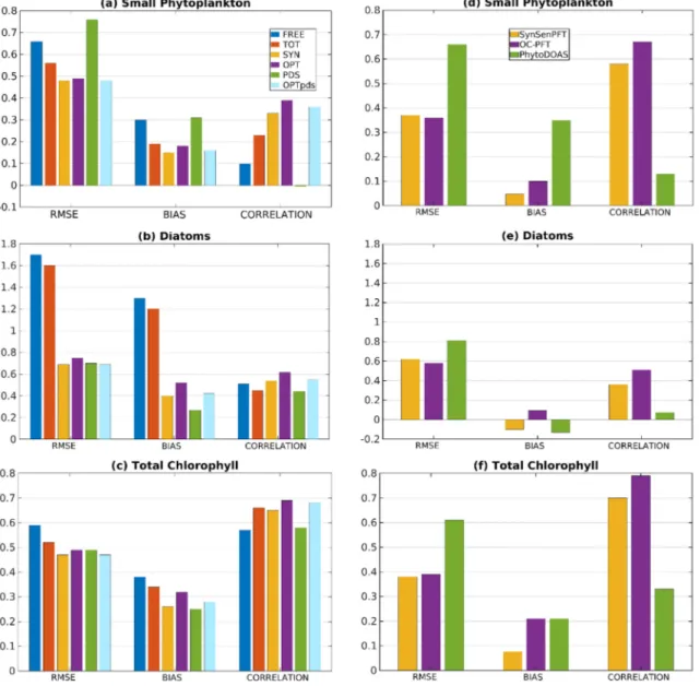
To evaluate the assimilation results with less dependent data, Figures 2a–2c show the RMSE and mean error (bias) computed from modelfields minus in situ data, and the correlation coefficient for the matchup points.

All diagnostics are computed for logarithmic concentrations with regard to the in situ data for SP, diatoms, and TChla. Comparing the left three bars in each group, which show the experiments FREE, TOT, and SYN, one sees the general effect of assimilating PFT data. The assimilation of TChla in experiment TOT reduces the RMSE and bias for SP and diatoms compared to FREE by about 0.1. Further the correlation is increased for SP from 0.1 to 0.23, while it is slightly decreased from 0.51 to 0.45 for diatoms. The PFT assimilation in the experiment SYN further reduces the RMSE and bias. The error reduction is small for SP (14% for RMSE and 21% for bias) but much larger for the diatoms where the RMSE for diatoms is reduced by about 57%, and the bias is reduced by 67% compared to TOT. The correlation is increased in SYN to 0.33 for SP and 0.54 for dia- toms, so that in SYN also the correlation for diatoms is higher than in FREE. The effect on the TChla is shown in Figure 2c. When PFT data are assimilated, the RMSE and bias are reduced compared to the assim- ilation of TChla in experiment TOT. Further, the correlation is increased in the experiments OPT and

Figure 1.Chlorophyll concentration of small phytoplankton (left column) and diatoms (right column) for 20 April 2009: (a, b) experiment TOT: assimilation of TChla, (c, d) experiment SYN: assimilation of SynSenPFT type data, and (e, f) difference SYN‐TOT of the concentrations.

Table 1

RMS Errors of Logarithmic Chlorophyll Concentrations for Small Phytoplankton, Diatoms, and Total Chlorophyll With Regard to SynSenPFT Data for the Global Model Domain and Five Regions for the Free Run (FREE), Total Chlorophyll Assimilation (TOT), and PFT Assimilation of SynSenPFT Data (SYN)

Small phytoplankton Diatoms Total chlorophyll

FREE TOT SYN FREE TOT SYN FREE TOT SYN

Global 0.609 0.507 0.408 1.96 1.71 0.799 0.558 0.44 0.401

Northern 0.948 0.901 0.663 1.77 1.44 0.739 0.739 0.597 0.584

NCR 0.47 0.390 0.355 2.11 1.88 0.805 0.445 0.368 0.339

Equatorial 0.427 0.281 0.268 1.91 1.65 0.831 0.5 0.353 0.32

SCR 0.417 0.318 0.293 2.2 1.99 0.881 0.445 0.352 0.314

Antarctic 0.77 0.649 0.478 1.66 1.42 0.628 0.664 0.502 0.451

Note. The numbers in bold mark the smallest RMSE.

Figure 2.(left column) RMSE, bias, and correlation for model experiments with regard to in situ observations computed for logarithmic concentrations of (a) small phytoplankton (b) diatoms, and (c) total chlorophyll. The values are shown for the free run (FREE), the assimilation of total chlorophyll (TOT), and four cases of PFT assimilation (SYN, OPT, PDS, and OPTpds). (right column) RMSE, bias, and correlation for satellite data with in situ observations of (d) small phytoplankton, (e) diatoms, (f) total chlorophyll for SynSenPFT, OC‐PFT, and PhytoDOAS.

OPTpds but decreased in SYN and PDS. Thus, the assimilation of PFT data is overall also beneficial for the representation of TChla.

3.2. Assimilation Effect of Different PFT Data Sets

Figures 2a–c show also the RMSE, bias, and correlation coefficient for all four experiments with assimilation of PFT data (right four bars in each group). For SP, the experiment PDS which assimilated the PhytoDOAS data has a higher RMSE and bias, and nearly zero correlation. This is different for diatoms, where the RMSE is comparable with that of the experiments that assimilated PFT data and the bias is particularly low. For the other three experiments, the RMSE and bias for SP are nearly the same (lowest for SYN, then OPTpds and then OPT) and the correlation is highest for OPT (0.39) and nearly the same, 0.33 and 0.36, respectively, for SYN and OPTpds. When we compare the experiment OPT with OPTpds, we see that the additional assimila- tion of PhytoDOAS data leads to small reductions in the RMSE and bias, and also a smaller correlation for both SP and diatoms.

Figures 2d–2f show the diagnostics for the satellite data compared to the in situ data. Here the total number of collocation points for SP, diatoms, and TChla are 646, 450, and 802, respectively. The points are fewer because the satellite data values are only available above 0.01 mg/m³. For these points, the RMSE and bias are lower and the correlation is higher for SP and TChla compared to the model results. For diatoms, the bias for the satellite data is close to zero. However, the RMSE is only slightly lower for the satellite data and the correlation is slightly higher for the model.

3.3. Assimilation Effect on Phytoplankton Community Structure

The changes to the SP and diatoms caused by the data assimilation lead to changes in the phytoplankton community structure. To discuss the effect, Figure 3 shows the fraction of SP in the total chlorophyll aver- aged over April 2009 as a compact representation of the community structure. Yellow to red colors show that the SP are dominant, while green to blue colors indicate a dominance of diatoms. The free run (Figure 3a) shows dominance by diatoms in the North Pacific and North Atlantic oceans, in the Weddell Sea, and to a lesser degree in the Ross Sea. All other areas are strongly dominated by SP. When total chlorophyll is assimi- lated (Figure 3b), diatoms become more dominant in the Southern Ocean south of 60°S. On the other hand, the dominance of diatoms is reduced in the North Pacific and Atlantic.

The PFT assimilation in the experiments SYN and OPTpds, shown in Figures 3c and 3d, respectively (simi- lar in OPT, not shown), leads to an overall reduction of the dominances. Thus, while the dominance of SP in FREE and TOT is nearly 100% in regions where SP dominates, this dominance is reduced in SYN to a level of 85 to 90%. This effect is analogous for the regions where diatoms dominate. The PFT assimilation changes the dominance pattern in the Southern Ocean to a lesser degree than the assimilation of TChla.

The major change is a switch from dominance of SP to diatoms inside the Ross Sea. In the North Pacific, the PFT assimilation reduces the overall dominance of diatoms similar to the experiment TOT.

A large difference between TOT and SYN or OPTpds is visible in the North Atlantic. Here SP becomes dominant north of 60°N in wide parts of the ocean, while in TOT the dominance of diatoms was only reduced to a small degree. Comparing SYN (Figure 3c) with OPTpds (Figure 3d) we see that both cases lead to very similar dominance distributions. Mainly, the dominance of SP is about 5–10% lower in OPTpds, in particular in the Northern Hemisphere. Larger differences only occur in the Norwegian Sea, the Kara Sea, and the Labrador Sea where the dominance of SP is partly higher for SYN than OPTpds. In the northern basin and the Antarctic basin, the assimilation has the effect to reduce the seasonal variability of domi- nance. Thus, while in the experiment FREE the diatoms clearly dominate the whole region in later winter and early spring and SP dominates during summer on both hemispheres, the PFT assimilation reduces the strength of the dominance (not shown). In consequence, while there are still locations in these regions in which diatoms dominate during the early spring blooms, there is no clear dominance any more on the regional average (not shown).

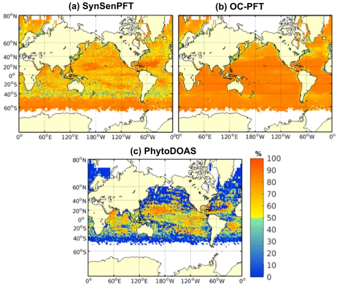
Figure 4 depicts the dominance of PFTs from satellite data averaged over April 2009. The SynSenPFT data show nearly the same spatial distribution as OC‐PFT data except in the region around 40°S where diatoms dominate in the SynSenPFT data. There is a stronger dominance of SP in the OC‐PFT data in general. The dominance of diatoms in the regions around Cape Verde, Yellow Sea, Barents Sea, and eastern Labrador Sea is visible in both satellite data sets. PhytoDOAS data (Figure 4c) show a distinct dominance pattern with

much wider diatoms dominance in comparison to SynSenPFT and OC‐PFT data. The assimilation of PFT data is able to bring the community structure closer to the features seen in SynSenPFT and OC‐PFT data.

However, the dominance level of SP is still higher and the dominance of diatoms around 40°S (Figure 4a) and around Cape Verde is not present in the assimilation. The assimilation also improved the consistency of the community structure when compared to the in situ data. Analogous to the scores shown in Figure 2, the RMSE and bias were reduced from 0.4 and 0.21 in FREE (figure not shown) to 0.29 and 0.11, respectively, in the experiment SYN. The correlation was only slightly improved from 0.26 in FREE to 0.3 in SYN.

4. Discussion

Comparing the assimilation of TChla with the assimilation of PFT data in section 3.1 it is evident that the assimilation of satellite PFT data in particular improves the representation of diatoms. Pradhan et al.

(2019) showed that the use of the ensemble‐estimated cross covariance in the assimilation of TChla already leads to a better representation of diatoms, compared to the assimilation approach that preserves the ratio of each group to TChla (as, e.g., used by Nerger & Gregg, 2008; Gregg, 2008; Rousseaux & Gregg, 2015).

However, assimilating TChla data, the RMSEs for diatoms computed with regard to SynSenPFT satellite data and with regard to in situ data are still much higher than the RMSEs for SP. This error is strongly reduced when PFT satellite data are assimilated. In the evaluation with situ data, the PFT assimilation leads to smaller RMSE and bias, and a larger correlation than the assimilation of TChla for both SP and diatoms, and also the estimated TChla. This holds for all experiments, except when assimilating only PhytoDOAS Figure 3.Fraction of small phytoplankton in the total chlorophyll averaged over April 2019. Green to blue colors show that diatoms are dominant, while small phytoplankton dominates for yellow to red colors. Shown are the fraction for the (a) FREE: free run, (b) TOT: total chlorophyll assimilation, (c) SYN:

SynSenPFT assimilation, and (d) OPTpds: joint assimilation of OC‐PFT and PhytoDOAS data.

data, even though the SP represented in the model does not fully coincide with the PFTs included in the data sets (e.g., haptophytes and cyanobacteria, whose sum was used to represent SP). This positive influence of PFT data is consistent with thefindings of Ciavatta et al. (2018), who assimilated PFTs into a regional model of the North East Atlantic.

The experiment TOT used varying observation errors, while the SYN usedfixed errors. To assess the impact of the varying errors, we have repeated the experiment TOT with afixed observation error of 0.3. When com- paring with SynSenPFT data, the RMSE for the TChla was reduced, that is, the assimilation had an overall stronger effect on TChla. However, for the SP this led to mixed results with regional increases and decreases in the range of ± 13% while the representation of diatoms was regionally deteriorated by up to 23%.

However, in the evaluation with the in situ data, the change in the assumed observation error had a negligible effect.

When the different PFT data sets are assimilated, the differences are smaller than the difference to the assim- ilation of TChla. However, assimilating only PhytoDOAS in experiment PDS leads to higher errors for SP than in the other experiments. This can be partly attributed to a lower data coverage of PhytoDOAS com- pared to OC‐PFT data. However, the PhytoDOAS data itself also show higher RMS error and bias with regard to the in situ data than the OC‐PFT data. The influence of PhyotoDOAS data is clearly different for diatoms, where the assimilation of PhytoDOAS data leads to the smallest bias of all experiments with regard to in situ data. Thus, for diatoms, the PhytoDOAS data provide useful information despite the smaller data availability than OC‐PFT.

Figure 4.Same as Figure 3 but for satellite data averaged over April 2009 for (a) SynSenPFT, (b) OC‐PFT, (c) PhytoDOAS data.

Both experiments that assimilated either SynSenPFT data (SYN) or jointly OC‐PFT and PhytoDOAS data (OPTpds) use these two types of PFT data. In SynSenPFT they are empirically combined and then assimi- lated, while in the experiment OPTpds the uncertainty and covariance estimated from the ensemble simula- tion are used to assimilate the separate data sets at once. While the evaluation with in situ data shows that the errors of SP and diatoms are very similar for both cases, the joint assimilation resulted in higher correla- tions than the assimilating SynSenPFT data.

The assimilation of different PFT data sets also had an effect on the phytoplankton community structure.

The dominance of SP, which is present in wide parts of the ocean, was only slightly reduced with the joint assimilation in OPTpds compared to the assimilation of SynSenPFT data. This shows that the diatoms data have a stronger influence in the assimilation experiment OPTpds where it is directly used compared to when it is assimilated as a combined data set in SynSenPFT. This is associated with the stronger reduction of the diatoms bias visible in Figure 2. Thus, this study would be helpful for validating projections of future changes in phytoplankton community structure where dominance is a useful indicator for representing the community.

In general, one has to keep in mind that the following also adds to the uncertainty in the comparison of free run, assimilated and satellite product: all assimilated PFT products represent the diatoms, but the SP is represented by combinations of different phytoplankton types. PhytoDOAS data contain only cyanobacteria (prokaryotic phytoplankton) and coccolithophores, while the OC‐PFT data and also the in situ PFT data cover haptophytes and prokaryotic phytoplankton. This is in contrast to the model in which SP represents all the phytoplankton except the diatoms. Further, the OC‐PFT and SynSenPFT data sets were based on OC‐CCI data in version 2, while the assimilated OC‐CCI data were version 3.1. The differences in the two versions are not large, but the comparison of the effect is not exact. However, we expect that the differences in the effects on the PFTs when assimilating TChla data (experiment TOT) compared to assimilating PFTs in the other experiments are much larger than the effect of different versions of OC‐CCI data.

5. Conclusion

An increasing number of biogeochemical models represent more than one plankton functional type in their phytoplankton and use those to predict quantities that have some relation to the composition of the phyto- plankton pool, not only its biomass. An example is the prediction of the production of dimethylsulfide, a component primarily produced by haptophyte algae, such as coccolithophores orPheocystis spp. (Vogt et al., 2010). It has been questioned, however, how robust the predictions of PFT models are, due to their lar- ger number of not‐so‐well constrained parameters that describe PFT growth or mortality (Anderson, 2005).

It is therefore of high interest, whether assimilating PFT data derived from satellite observations helps in bet- ter constraining these models.

In this work, satellite data of PFTs were assimilated into the ocean‐biogeochemical model MITgcm‐REcoM2 over the years 2008 and 2009 and the effect of different data products was assessed. Overall, the assimilation experiments show that the assimilation of satellite data of PFTs can improve their model representation compared to the case when only TChla data are assimilated. In the case of a global model with two PFTs used here, the diatoms group was improved to a large degree while the improvement of the SP group was smaller.

A reason for this might be that the SP group in the model is not exactly represented by the assimilated PFT data, and also the in situ data used to assess the assimilation results did not exactly represent the model SP group. This indicates that it is important to have PFT data thatfit the groups in the model. In the study by Ciavatta et al. (2018), the PFT data were particularly generated to be consistent with their model, while here, readily available data sets were used. However, the satellite PFT data sets used in Ciavatta et al. (2018), and likewise the OC‐PFT data set used in our study, are retrieved using empirically derived relationships between total chlorophyll and PFTs. Hence, these data sets will have higher errors than the TChla data itself.

The difference in the state estimates when different PFT data products are assimilated is much smaller than the difference for TChla assimilation. However, assimilating PhytoDOAS data led to higher errors for small phytoplankton. A joint assimilation of OC‐PFT and PhytoDOAS data improved the simulation decreasing the RMS errors and bias in comparison to assimilating only OC‐PFT data. The joint assimilation and the assimilation of the synergistically combined data product SynSenPFT led to very similar RMS error and bias, but the correlation was slightly higher for the joint assimilation. This indicates that assimilating the data

products separately might be beneficial as the data assimilation combines the observational information using the covariances that are dynamically estimated by the ensemble; however, the difference was not significant here.

The PFT assimilation performed here has several limitations. First, it was performed with estimated con- stant observation errors because no error information was provided with the PFT data sets. Further, the spa- tial resolution and temporal availability of the data limit its influence in the data assimilation. This holds especially for PhytoDOAS data that has only weekly coverage, which is much lower than the daily availabil- ity of the SynSenPFT and OC‐PFT products. However, despite its lower coverage, assimilating the PhytoDOAS data next to OC‐PFT data was still beneficial for the representation of the diatoms. Further improvements are expected from data sets whose PFTs are consistent with those represented by the model, by improved data coverage, and by availability of spatially varying observational errors. Further, as a possi- ble future work one could combine OC‐PFT and PhytoDOAS data using different error variances for each in the assimilation, and/or performing bias correction between the products.

The data assimilation methodology applied here used the logarithm of the chlorophyll concentrations.

While the lognormal distribution is a common assumption, it might not be fully true. This is indicated by the sensitivity of the data assimilation process, which was stabilized here using a vertical localization and a limitation of the maximum assimilation increment. It is a task for the future to study whether using the so‐called Gaussian anamorphosis of the ensemble, for example, used by Doron et al. (2011), can lead to a bet- ter ensemble distribution for the computation of the data assimilation increments.

References

Aiken, J., Fishwick, J. R., Lavender, S., Barlow, R., Moore, G. F., Sessions, H., et al. (2007). Validation of MERIS reflectance and chlorophyll during the BENCAL cruise October 2002: Preliminary validation of new demonstration products for phytoplankton functional types and photosynthetic parameters.International Journal of Remote Sensing,28(3–4), 497–516. https://doi.org/10.1080/

01431160600821036

Anderson, T. R. (2005). Plankton functional type modelling: Running before we can walk?Journal of Plankton Research,27(11), 1073–1081.

https://doi.org/10.1093/plankt/fbi076

Aumont, O., Ethé, C., Tagliabue, A., Bopp, L., & Gehlen, M. (2015). PISCES‐v2: An ocean biogeochemical model for carbon and ecosystem studies.Geoscientific Model Development,8(8), 2465–2513. https://doi.org/10.5194/gmd‐8‐2465‐2015

Balch, W. M., Gordon, H. R., Bowler, B. C., Drapeau, D. T., & Booth, E. S. (2005). Calcium carbonate measurements in the surface global ocean based on Moderate‐Resolution Imaging Spectroradiometer data.Journal of Geophysical Research,110, C07001. https://doi.org/

10.1029/2004JC002560

Bracher, A., Dinter, T., Wolanin, A., Rozanov, V., Vladimir, V., Losa, S. N., & Soppa, M. A. (2017). Global monthly mean chlorophyll“a”

surface concentrations from August 2002 to April 2012 for diatoms, coccolithophores and cyanobacteria from PhytoDOAS algorithm version 3.3 applied to SCIAMACHY data, link to NetCDFfiles in ZIP archive. PANGAEA. https://doi.org/10.1594/PANGAEA.870486 Bracher, A., Vountas, M., Dinter, T., Burrows, J. P., Röttgers, R., & Peeken, I. (2009). Quantitative observation of cyanobacteria and diatoms

from space using PhytoDOAS on SCIAMACHY data.Biogeosciences,6(5), 751–764. https://doi.org/10.5194/bg‐6‐751‐2009

Brewin, R. J. W., Ciavatta, S., Sathyendranath, S., Jackson, T., Tilstone, G., Curran, K., et al. (2017). Uncertainty in ocean‐color estimates of chlorophyll for phytoplankton groups.Frontiers in Marine Science,4. https://doi.org/10.3389/fmars.2017.00104

Brewin, R. J. W., Sathyendranath, S., Jackson, T., Barlow, R., Brotas, V., Airs, R., & Lamont, T. (2015). Influence of light in the mixed‐layer on the parameters of a three‐component model of phytoplankton size class.Remote Sensing of Environment,168, 437–450. https://doi.

org/10.1016/J.RSE.2015.07.004

Campbell, J. W. (1995). The lognormal distribution as a model for bio‐optical variability in the sea.Journal of Geophysical Research, 100(C7), 13,237. https://doi.org/10.1029/95JC00458

Chen, Z., Liu, J., Song, M., Yang, Q., & Xu, S. (2017). Impacts of assimilating satellite sea ice concentration and thickness on Arctic sea ice prediction in the NCEP climate forecast system.Journal of Climate,30(21), 8429–8446. https://doi.org/10.1175/JCLI‐D‐17‐0093.1 Ciavatta, S., Brewin, R. J. W., Skákala, J., Polimene, L., de Mora, L., Artioli, Y., & Allen, J. I. (2018). Assimilation of ocean‐color plankton

functional types to improve marine ecosystem simulations.Journal of Geophysical Research: Oceans,123, 834–854. https://doi.org/

10.1002/2017JC013490

Ciavatta, S., Kay, S., Saux‐Picart, S., Butenschön, M., & Allen, J. I. (2016). Decadal reanalysis of biogeochemical indicators andfluxes in the North West European shelf‐sea ecosystem.Journal of Geophysical Research: Oceans,121, 1824–1845. https://doi.org/10.1002/

2015JC011496

Ciavatta, S., Torres, R., Saux‐Picart, S., & Allen, J. I. (2011). Can ocean color assimilation improve biogeochemical hindcasts in shelf seas?

Journal of Geophysical Research,116, C12043. https://doi.org/10.1029/2011JC007219

Doron, M., Brasseur, P., & Brankart, J.‐M. (2011). Stochastic estimation of biogeochemical parameters of a 3D ocean coupled physical–

biogeochemical model: Twin experiments.Journal of Marine Systems,87(3), 194–207. https://doi.org/10.1016/j.jmarsys.2011.04.001 Dutkiewicz, S., Hickman, A. E., Jahn, O., Gregg, W. W., Mouw, C. B., & Follows, M. J. (2015). Capturing optically important constituents

and properties in a marine biogeochemical and ecosystem model.Biogeosciences,12(14), 4447–4481. https://doi.org/10.5194/bg‐12‐4447‐ 2015

Evensen, G. (1994). Sequential data assimilation with a nonlinear quasi‐geostrophic model using Monte Carlo methods to forecast error statistics.Journal of Geophysical Research,99(C5), 10,143. https://doi.org/10.1029/94JC00572

Ford, D., & Barciela, R. (2017). Global marine biogeochemical reanalyses assimilating two different sets of merged ocean colour products.

Remote Sensing of Environment,203, 40–54. https://doi.org/10.1016/j.rse.2017.03.040 Acknowledgments

We acknowledge the North‐German Supercomputing Alliance (HLRN) for providing HPC resources that have contributed to the research results reported in this paper. This work is funded by the AWI Strategy Fund of the Alfred Wegener Institute Helmholtz Centre for Polar and Marine Research (AWI), Germany. We acknowledge the Euromarine network for funding par- tially to attend the“Ensemble data assimilation workshop 2016”in Bergen, Norway, which gave H. K. P. deeper insight regarding assimilation. S. L.

gratefully acknowledges the funding by the Deutsche Forschungsgemeinschaft (DFG, German Research Foundation)

—project 268020496—TRR 172, within the Transregional Collaborative Research Center“ArctiC Amplification: Climate Relevant Atmospheric and SurfaCe Processes, and Feedback Mechanisms (AC)3”and partly made in the framework of the state assignment of the Federal Agency for Scientific Organizations (FASO) Russia (theme 0149‐2019‐0015). The in situ data for validation are available at https://doi.pangaea.de/10.1594/

PANGAEA.875879 while the model simulations are available at https://doi.

pangaea.de/10.1594/

PANGAEA.910973. Finally, the authors would like to acknowledge the two anonymous reviewers for their con- structive comments.

Gehlen, M., Barciela, R., Bertino, L., Brasseur, P., Butenschön, M., Chai, F., et al. (2015). Building the capacity for forecasting marine biogeochemistry and ecosystems: Recent advances and future developments.Journal of Operational Oceanography,8(sup1), s168–s187.

https://doi.org/10.1080/1755876X.2015.1022350

Geider, R. J., MacIntyre, H. L., & Kana, T. M. (1998). A dynamic regulatory model of phytoplanktonic acclimation to light, nutrients, and temperature.Limnology and Oceanography,43(4), 679–694. https://doi.org/10.4319/lo.1998.43.4.0679

Goodliff, M., Bruening, T., Schwichtenberg, F., Li, X., Lindenthal, A., Lorkowski, I., & Nerger, L. (2019). Temperature assimilation into a coastal ocean‐biogeochemical model: Assessment of weakly and strongly coupled data assimilation.Ocean Dynamics,69(10), 1217–1237. https://doi.org/10.1007/s10236‐019‐01299‐7

Gregg, W. W. (2008). Assimilation of SeaWiFS ocean chlorophyll data into a three‐dimensional global ocean model.Journal of Marine Systems,69(3–4), 205–225. https://doi.org/10.1016/j.jmarsys.2006.02.015

Gregg, W. W., Ginoux, P., Schopf, P. S., & Casey, N. W. (2003). Phytoplankton and iron: Validation of a global three‐dimensional ocean biogeochemical model.Deep Sea Research Part II: Topical Studies in Oceanography,50(22), 3143–3169. https://doi.org/10.1016/j.

dsr2.2003.07.013

Gregg, W. W., & Rousseaux, C. S. (2014). Decadal trends in global pelagic ocean chlorophyll: A new assessment integrating multiple satellites, in situ data, and models.Journal of Geophysical Research: Oceans,119, 5921–5933. https://doi.org/10.1002/

2014JC010158

Hardman‐Mountford, N. J., Hirata, T., Richardson, K. A., & Aiken, J. (2008). An objective methodology for the classification of ecological pattern into biomes and provinces for the pelagic ocean.Remote Sensing of Environment,112(8), 3341–3352. https://doi.org/10.1016/j.

rse.2008.02.016

Hauck, J., Völker, C., Wang, T., Hoppema, M., Losch, M., & Wolf‐Gladrow, D. A. (2013). Seasonally different carbonflux changes in the Southern Ocean in response to the southern annular mode.Global Biogeochemical Cycles,27, 1236–1245. https://doi.org/10.1002/

2013GB004600

Hirata, T., Hardman‐Mountford, N. J., Brewin, R. J. W., Aiken, J., Barlow, R., Suzuki, K., et al. (2011). Synoptic relationships between surface Chlorophyll‐aand diagnostic pigments specific to phytoplankton functional types.Biogeosciences,8(2), 311–327. https://doi.org/

10.5194/bg‐8‐311‐2011

Hohn, S. (2009). Coupling and decoupling of biogeochemical cycles in marine ecosystems.Ecological Modelling,135.

Large, G., & Yeager, S. (2004). Diurnal to decadal global forcing for ocean and sea‐ice models: The data sets andflux climatologies. https://

doi.org/10.5065/D6KK98Q6

Laws, E. A., & Bannister, T. T. (2004). Nutrient‐and light‐limited growth ofThalassiosirafluviatilisin continuous culture with implications for phytoplankton growth in the ocean. Retrieved November 6, 2019, from https://aslopubs.onlinelibrary.wiley.com/doi/abs/10.4319/

lo.2004.49.6.2316

Le Quéré, C. L., Harrison, S. P., Colin Prentice, I., Buitenhuis, E. T., Aumont, O., Bopp, L., et al. (2005). Ecosystem dynamics based on plankton functional types for global ocean biogeochemistry models.Global Change Biology,11(11), 2016–2040. https://doi.org/10.1111/

j.1365‐2486.2005.1004.x

Losa, S. N., Soppa, M., Dinter, T., Wolanin, A., Oelker, J., & Bracher, A. (2017b). Global chlorophyllasurface concentrations for diatoms, coccolithophores and cyanobacteria as the synergistic SynSenPFT product combined PhytoDOAS and OC‐PFT for the period of time August 2002–April 2012, links to NetCDFfiles. PANGAEA. https://doi.org/10.1594/PANGAEA.875873. Supplement to: Losa, S. N. et al.

(2017): Synergistic exploitation of hyper‐and multi‐spectral precursor sentinel measurements to determine phytoplankton functional types (SynSenPFT). Frontiers in Marine Science, 4, 203. https://doi.org/10.1594/PANGAEA.875873

Losa, S. N., Soppa, M. A., Dinter, T., Wolanin, A., Brewin, R. J. W., Bricaud, A., et al. (2017a). Synergistic exploitation of hyper‐and multi‐

spectral precursor sentinel measurements to determine phytoplankton functional types (SynSenPFT).Frontiers in Marine Science,4, 203. https://doi.org/10.3389/fmars.2017.00203

Losch, M., Menemenlis, D., Campin, J.‐M., Heimbach, P., & Hill, C. (2010). On the formulation of sea‐ice models. Part 1: Effects of different solver implementations and parameterizations.Ocean Modelling,33(1), 129–144. https://doi.org/10.1016/j.ocemod.2009.12.008 Mahowald, N. (2003). Interannual variability in atmospheric mineral aerosols from a 22‐year model simulation and observational data.

Journal of Geophysical Research,108(D12), 4352. https://doi.org/10.1029/2002JD002821

Maritorena, S., D'Andon, O. H. F., Mangin, A., & Siegel, D. A. (2010). Merged satellite ocean color data products using a bio‐optical model:

Characteristics, benefits and issues.Remote Sensing of Environment,114(8), 1791–1804. https://doi.org/10.1016/J.RSE.2010.04.002 MITgcm Group. (2018). MITGCM USER MANUAL. Retrieved from http://mitgcm.org/public/r2_manual/latest/online_documents/

manual.html

Mu, L., Losch, M., Yang, Q., Ricker, R., Losa, S. N., & Nerger, L. (2018). Arctic‐wide sea ice thickness estimates from combining satellite remote sensing data and a dynamic ice‐ocean model with data assimilation during the CryoSat‐2 period.Journal of Geophysical Research:

Oceans,123, 7763–7780. https://doi.org/10.1029/2018JC014316

Natvik, L.‐J., & Evensen, G. (2003). Assimilation of ocean colour data into a biochemical model of the North Atlantic: Part 1. Data assimilation experiments.Journal of Marine Systems,40–41, 127–153. https://doi.org/10.1016/S0924‐7963(03)00016‐2

Nerger, L., & Gregg, W. W. (2007). Assimilation of SeaWiFS data into a global ocean biogeochemical model using a local SEIKfilter.Journal of Marine Systems,68(301), 237–254.

Nerger, L., & Gregg, W. W. (2008). Improving assimilation of SeaWiFS data by the application of bias correction with a local SEIKfilter.

Journal of Marine Systems,73(1–2), 87–102. https://doi.org/10.1016/J.JMARSYS.2007.09.007

Nerger, L., & Hiller, W. (2013). Computers & geosciences software for ensemble‐based data assimilation systems—Implementation stra- tegies and scalability.Computers and Geosciences,55, 110–118. https://doi.org/10.1016/j.cageo.2012.03.026

Nerger, L., Janjić, T., Schröter, J., & Hiller, W. (2012). A regulated localization scheme for ensemble‐based Kalmanfilters.Quarterly Journal of the Royal Meteorological Society,138(664), 802–812. https://doi.org/10.1002/qj.945

Ourmières, Y., Brasseur, P., Lévy, M., Brankart, J. M., & Verron, J. (2009). On the key role of nutrient data to constrain a coupled physical‐

biogeochemical assimilative model of the North Atlantic Ocean.Journal of Marine Systems,75(1–2), 100–115. https://doi.org/10.1016/j.

jmarsys.2008.08.003

Pradhan, H. K., Völker, C., Losa, S. N., Bracher, A., & Nerger, L. (2019). Assimilation of global total chlorophyll OC‐CCI data and its impact on individual phytoplanktonfields.Journal of Geophysical Research: Oceans,124, 470–490. https://doi.org/10.1029/2018JC014329 Rousseaux, C. S., & Gregg, W. W. (2012). Climate variability and phytoplankton composition in the Pacific Ocean.Journal of Geophysical

Research,117, C10006. https://doi.org/10.1029/2012JC008083

Rousseaux, C. S., & Gregg, W. W. (2015). Recent decadal trends in global phytoplankton composition.Global Biogeochemical Cycles,29, 1674–1688. https://doi.org/10.1002/2015GB005139