https://doi.org/10.5194/bg-18-1351-2021
© Author(s) 2021. This work is distributed under the Creative Commons Attribution 4.0 License.
Technical note: Seamless gas measurements across the land–ocean aquatic continuum – corrections and evaluation of sensor data for CO 2 , CH 4 and O 2 from field deployments in contrasting environments
Anna Rose Canning1,2,a, Peer Fietzek3, Gregor Rehder4, and Arne Körtzinger1,5
1GEOMAR Helmholtz-Zentrum für Ozeanforschung, Kiel, Germany
2-4H- JENA engineering GmbH, Jena, Germany
3Kongsberg Maritime GmbH, Hamburg, Germany
4Leibniz Institute for Baltic Sea Research Warnemünde, Rostock–Warnemünde, Germany
5Christian-Albrechts-Universität zu Kiel, Kiel, Germany
aformerly at: Kongsberg Maritime Contros GmbH, Kiel, Germany Correspondence:Anna Rose Canning (acanning@geomar.de) Received: 16 April 2020 – Discussion started: 4 May 2020
Revised: 2 November 2020 – Accepted: 18 November 2020 – Published: 23 February 2021
Abstract. The ocean and inland waters are two separate regimes, with concentrations in greenhouse gases differing on orders of magnitude between them. Together, they cre- ate the land–ocean aquatic continuum (LOAC), which com- prises itself largely of areas with little to no data with re- gards to understanding the global carbon system. Reasons for this include remote and inaccessible sample locations, often tedious methods that require collection of water sam- ples and subsequent analysis in the lab, and the complex in- terplay of biological, physical and chemical processes. This has led to large inconsistencies, increasing errors and has in- evitably lead to potentially false upscaling. A set-up of mul- tiple pre-existing oceanographic sensors allowing for highly detailed and accurate measurements was successfully de- ployed in oceanic to remote inland regions over extreme concentration ranges. The set-up consists of four sensors si- multaneously measuring pCO2, pCH4 (both flow-through, membrane-based non-dispersive infrared (NDIR) or tunable diode laser absorption spectroscopy (TDLAS) sensors), O2
and a thermosalinograph at high resolution from the same water source. The flexibility of the system allowed for de- ployment from freshwater to open ocean conditions on vary- ing vessel sizes, where we managed to capture day–night cy- cles, repeat transects and also delineate small-scale variabil- ity. Our work demonstrates the need for increased spatiotem-
poral monitoring and shows a way of homogenizing methods and data streams in the ocean and limnic realms.
1 Introduction
Both carbon dioxide (CO2) and methane (CH4) are sig- nificant players in the Earth’s climate system, with 2016 being the first full year in which atmospheric CO2 rose above 400 parts per million (ppm), with an average of 402.8±0.1 ppm (Le Quéré et al., 2018). Since 1750, it has risen from 277 ppm. A similar trend has been seen with CH4, which has increased by 150 % in the atmosphere to 1803 parts per billion (ppb) between 1750 and 2011 (Ciais et al., 2013), with an acceleration in recent years to 1850 ppb in 2017 (Nisbet et al., 2019). With the oceans being a sink for an estimated ∼24 % of anthropogenic CO2 emissions (Friedlingstein et al., 2019), they have been under continu- ous observation and study, resulting in the collection of large global databases (e.g., Takahashi et al., 2009; Bakker et al., 2016). Such observations have shown both regional and/or temporal variabilities between a source and sink for CO2, yet it is typically a low to moderate CH4 source (∼0.4–
1.8 Tg CH4yr−1; Bates et al., 1996; Borges et al., 2018; Rhee 2009), increasing in coastal regions (Bange, 2006). Inland
waters, however, are a different story, and although it has been known for over 50 years that they are mostly supersat- urated with CO2(Park, 1969), up until recently their budgets have been of relatively little focus. Although regions such as lakes, rivers and reservoirs have been recognized as sig- nificant players in the carbon budget over the past couple of decades (see Carpenter et al., 1995; Cole and Caraco, 1998;
Caraco, 2001 with updates and reviews from Tranvik et al., 2009; Raymond et al., 2013 and Regnier et al., 2013), com- pared to the ocean data sets, having quantified and consistent data and consensus within these regions is still in the rel- atively early stages. Global CO2 and CH4 emissions from inland waters are estimated at 2.1 Pg C yr−1 (Raymond et al., 2013) and 0.7 Pg C yr−1(Bastviken et al., 2011), respec- tively. Mixing regimes (e.g. deltas and estuaries) and streams and smaller bodies of water are known to be overly impor- tant within these inland systems (Holgerson and Raymond, 2016; Natchimuthu et al., 2017; Grinham et al., 2018), yet there is very little data coverage with respect to both of these parameters (Borges et al., 2018) – even more so when they are evaluated together. Therefore, a specific need exists for high-resolution spatiotemporal measurements in regimes of highly dynamic, varyingpCO2concentrations (Yoon et al., 2016; Paulsen et al., 2018; Friedlingstein et al., 2019).
One issue leading to little data coverage is that the com- bination of both inland waters and the ocean, i.e. the land–
ocean aquatic continuum (LOAC), is usually not studied con- tinuously but rather split between oceanographers and lim- nologists. Although significant progress has been made in recognizing the importance of the LOAC as a whole sys- tem (e.g. Raymond et al., 2013; Regnier et al., 2013; Down- ing 2014; Palmer et al., 2015; Xenopoulos et al., 2017), huge knowledge gaps are still present, particularly related to limited field data availability (Meinson et al., 2016). Of- ten, this is due to different measuring techniques and pro- tocols, both with respect to in situ/autonomous observations and the collection of discrete data. This has been previously noted, through blind or spot sampling having large effects on the overall measured results, potentially leading to under- /overestimations in concentrations and fluxes (Richey et al., 2002; Abril et al., 2014; Canning et al., 2020b). Further- more, this is further complicated bypCO2,pCH4 and dis- solved O2being controlled by several factors, including bi- ological effects, vertical and lateral mixing and temperature- dependent thermodynamic effects (Bai et al., 2015). These effects are exacerbated within inland waters where variabil- ity is far higher due to variations in environmental conditions and the magnitude of biological processes and anthropogenic influences (Cole et al., 2007). The high spatial and tempo- ral variability within the inland/mixing waters (Wehrli, 2013) only increases these difficulties, ultimately leading to the in- terface between the ocean and inland to be considered one of the hardest systems to observe accurately and adequately.
This has led to limitations and lack of verifications, leading to errors, discrepancies and uncertainties involved in scaling up
the data. Inland waters tend to exhibit extreme ranges of CO2
partial pressure (pCO2,<100 to>10 000 µatm; this study;
Abril et al., 2015; Ribas-Ribas et al., 2011) in comparison to oceanic waters (∼100–700 µatm; Valsala and Maksyutov, 2010), while also showing extreme variabilities for both O2 and CH4. Given the much smaller concentration changes and gradients, oceanic sensors and methods have been specifi- cally tailored to assure high accuracy over oceanic concen- tration ranges, in comparison to inland waters.
One way of tackling these limitations and measurement technique differences is through sensors, ensuring a unified way of measuring with well-constrained accuracy and preci- sion. In specific regions, this has become more widespread and reviewed numerous times within the coastal and open ocean (see Atamanchuk et al., 2015; Clarke et al., 2017).
Multiple seagoing methods have been applied since the 1960s (see examples in Takahashi, 1961; DeGrandpre et al., 1995; Waugh et al., 2006; Pierrot et al., 2009; Schus- ter and Körtzinger, 2009; Becker et al., 2012) to measure and estimate greenhouse gases, such as CO2, across a vari- ety of aquatic regions. Inland water investigations have also seen clear progress with the development of continuous, au- tonomous measurement techniques (e.g. DeGrandpre et al., 1995; Baehr and DeGrandpre, 2004; Crawford et al., 2014;
Meinson et al., 2016; Brandt et al., 2017). Yet, only few studies have employed membrane-based equilibration sen- sors with non-dispersive infrared spectrometry (NDIR) de- tection (e.g. Johnson et al., 2009; Bodmer et al., 2016; Yoon et al., 2016; Hunt et al., 2017), with some adapting atmo- spheric sensors (see Bastviken et al., 2015). These methods often focus on only one gas (usually CO2), and none of these methods mentioned cover both water regimes (ocean to in- land), potentially leading to missed mixing regime regions.
On top of this, spatiotemporal data coverage has been noted to be sparse (Yoon et al., 2016) and is needed to advance our budget accuracies and understanding.
Given the biological and physical parameters of inland waters, multi-gas analyses is the way forward, which was previously noted in the work of Brennwald et al. (2016), where they worked on the development of the membrane in- let mass spectrometry (MIMS) known as miniRuedi. This system measured as a nearly fully autonomous multi-gas mass spectrometer; however, despite advances in both inert and reactive gas measurements, the need for a filter and gas standards for extreme gradients gives this set-up a disadvan- tage in highly diverse inland waters. This highlights one issue with extremely variable environments and shows that there is need to develop a robust, fully autonomous sensor system that is portable enough for small and simple platforms. The development needs to be able to measure a full range of con- centrations accurately and precisely, which is usually out of the specifications of sensors designed for one region. It needs to have the potential to measure multiple gases and ancillary parameters in unison across salinity and regional boundaries (including extreme concentrations), enabling us to measure
throughout the LOAC. These efforts would hopefully bridge the ocean–limnic gap both technically and by reducing dis- crepancies and errors while having high-resolution, real-time measurements. To be accepted within both inland waters and the ocean, it needs to be within oceanic specifications while being able to handle larger concentration ranges. This is es- sential for improved monitoring, potentially avoiding spot sampling bias, providing in-need high-quality spatiotemporal variability data, tracking the global carbon budget (Le Quéré et al., 2018) and potentially applying it in areas of the high- est uncertainties with potentially high anthropogenic input (Schimel et al., 2016).
Here we used state-of-the-art, membrane-based equilibra- tor non-dispersive infrared (NDIR) and tunable diode laser absorption spectroscopy (TDLAS) sensors for pCO2 and pCH4, respectively, which uses an oxygen optode and a ther- mosalinograph to create a set-up allowing measurements in a continuous flow-through system. To assess the versatility, performance, portability and measurement quality of the set- up, it was deployed across the three main aquatic environ- ments, namely oceanic, brackish and limnic. We present the technical findings from the campaigns, showing the need for such high-resolution combined gas data on a larger spatiotemporal scale; however, biogeochemical implications will not be further investigated. The primary objective of the work presented here was, with the use of oceanic, state-of- the-art tested sensors, to realize a fully versatile, portable and robust flow-through system to accurately, autonomously and simultaneously measure multiple dissolved gases (CO2, CH4
and O2) and ancillary parameters (temperature and salinity) across the full range of salinities. The second was to assess the potential for high-quality spatiotemporal data extraction.
The set-up was subsequently deployed in each region of se- lected salinities (ocean, brackish and limnic waters) to allow for both spatial and temporal measurements. Extensive post- campaign corrections were assessed to see the need for their adaptation over all the regions, and for the more precise cor- rections, small-scale variability was used. Discrete samples were collected, and reference systems were deployed along- side to provide quality assessment of the performance of the flow-through set-up.
2 Material and methods 2.1 Sensors and ranges
The set-up featured four separate sensors measuring three dissolved gases and standard hydrographic parameters (Ta- ble 1).
The CONTROS HydroC®CO2FT (HC–CO2) and CON- TROS HydroC® CH4 FT (HC–CH4) (formerly Kongsberg Maritime Contros GmbH, Kiel, Germany; now -4H- JENA Engineering GmbH, Jena, Germany, and hereinafter -4H- JENA) are both commercially manufactured sensors which
use membrane-based equilibrators combined with NDIR and TDLAS gas detectors, respectively. Both sensors are of the flow-through type in which water is pumped through a plenum, with a planar semi-permeable membrane, across which dissolved gas partial pressure equilibrium is estab- lished with the headspace behind, as described by Fietzek et al. (2014). The sensors were factory calibrated before and after each cruise (Romanian campaigns all together), and the calibration polynomials were provided (in case of thepCO2 sensor) by the manufacturer.
The CONTROS HydroFlash® O2 (formerly Kongsberg Maritime Contros GmbH, Kiel, Germany; hereinafter KM- CON) was an optical sensor (optode) based on the principle of fluorescence quenching (see Bittig et al., 2018b, for an op- tode technology review). As the sensor was only available as a submersible type, a flow-through cell was built around the sensor head for integration into the flow-through system.
The SBE 45 micro thermosalinograph (Sea-Bird Scien- tific, Bellevue, WA, USA) was used to measure temperature and conductivity to calculate salinity. All sensor frequencies depended on cruise type and were set between one reading output per minute to one reading per second (oceanic to in- land waters).
2.2 Initial procedures and background
Initial experiments were conducted within the laboratory at GEOMAR, Kiel, Germany, and during short sea trials on board research vessel (RV)Littorinain 2016 to ensure the optimal performance of all sensors (data not shown here).
HC–CO2was placed within the set-up upstream of HC–CH4
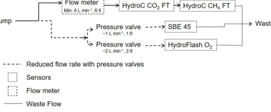
due to higher sensitivity and the dependence of the parame- terpCO2on temperature changes. The water flow was split between sensors, due to differing flow range requirements. A flow meter and pressure valves were installed to provide op- timal flow speeds, as shown in the schematic of the overall set-up (Fig. 1).
Depending on the vessel type and the location of the mea- surement system contained therein, the pump was placed either in the moon pool of the ship or at the front of the boat (limnic cruises; see Table 2). The total flow was reg- ulated by multiple pressure valves to a pump rate of approx- imately 9–10 L min−1. The HC–CO2and HC–CH4 show a distinct dependence on their response time (RT) and on the water flow rate, with the demand for the HC–CO2flow rates ranging from 2–16 L min−1(manufacturer recommendation is 5 L min−1) and flow rates for the HC–CH4ranging from 6–16 L min−1. Based on this information, combined with preliminary testing and power accessibility considerations across all regions, 6 L min−1was used as the target flow rate for the HC–CO2and HC–CH4. Data acquired with any flow rate below 5 L min−1were flagged as being questionable as they may have contributed to increased errors.
The data were logged on an internal logger for the HC–
CO2 and HC–CH4 in unison and displayed live using the
Figure 1.Flow schematic of the set-up, including minimal flow ratios. The flow rate was measured only for the main flow. For the side flows, the rate was adjusted, by pressure valves, to be a fraction (i.e. 1:9 and 2:9 for L min−1) of the total flow.
Table 1.Sensors and their manufacturer specifications, along with calibration range (for the CONTROS HydroC®CO2FT and CH4FT, factory calibration ranges were specific to the campaigns).
Model Deployment Detector Resolution Accuracy Response Specified Power Dimensions Weight Range of
type type time flow consumption (mm) (kg) factory
(t63) rate calibration
(min:sec) (L min−1)
CONTROS FTc <1 ±1 % t63∼1:32 350 mA 325x 0–6000
HydroC®CO2FT membrane NDIR µatm of at 16◦C; 2–15 at 240x 5.3 µatm
(-4H- JENA)a equilibration reading 5 L min−1 12 V 126
CONTROS FTc <0.01 ±2 µatm t63∼22:46 600 mA 452x <2−
HydroC®CH4FT membrane TDLAS µatm or 3 % at 17◦C; 6–15 at 283x 8.5 40 000
(-4H- JENA)a equilibration of reading 7 L min−1 12 V 142.5 µatm
CONTROS Fluorescence 0.1 J 23×197 0.17 air 0–400
HydroFlash®O2 Submersible quenching <0.1 % ±1 % t63<00:03 N/A per sample with 0.11 mbarpO2
(KMCON)b connector water
SBE 45d 30 mA at 338x 0 to 7
Thermosalinograph FTc Conductivity 0.00001 ±0.0003 N/A 0.6–1.8 12–30 V 134.4x 4.6 S m−1
Conductivity cell S m−1 S m−1 76.2
SBE 45d 30 mA at 338x −5 to
Thermosalinograph FTc Thermistor 0.0001 ±0.002 N/A 0.6–1.8 12–30 V 134.4x 4.6 +35◦C
Temperature ◦C ◦C 76.2
a-4H- JENA Engineering GmbH, Jena, Germany (formerly Kongsberg Maritime Contros GmbH, Kiel, Germany).bFormerly Kongsberg Maritime Contros GmbH, Kiel, Germany.
cFlow through.dSea-Bird Scientific, Bellevue, WA, USA.
CONTROS DETECT software. The SBE thermosalinograph and HydroFlash O2were logged on SeatermV2 software and a terminal programme (Tera Term), respectively. The sensors have the ability to set the timestamps for logged data, allow- ing alignment among all sensor systems and/or local time for discrete sample collection. Water flow was measured us- ing LabJack software, and any power cuts (or other circum- stances such as boats passing near to the house boat during the limnic cruises) were logged manually to ensure the best- quality outcome from the data processing which is described in the next sections.
The set-up was tested in the following three different lo- cations: the South Atlantic Ocean (oceanic), western Baltic Sea (brackish) and the Danube river delta, Romania, (limnic) between 2016 and 2017 (Figs. 2 and 3). Although, in brack- ish water regions like the Baltic Sea, the same measurement techniques for many instruments and sampling methods as
those within the ocean are used, certain techniques (e.g. al- kalinity titration) generally need special adaption for the low- salinity range. The different deployments ensured the sensors were tested in the field across the full salinity range, from freshwater to seawater, from moderate to tropical tempera- tures and from low concentrations near atmospheric equilib- rium to extreme cases of supersaturation (CH4and CO2) or undersaturation (CO2and O2). The choice of cruises also al- lowed testing of the versatility of the set-up by deploying it on a range of vessel types (see Fig. 2, Table 2 and Sect. 2.3).
2.3 Campaigns
2.3.1 Meteorcruise M133 to the South Atlantic (oceanic)
The system was set up on the RVMeteor(cruise M133) dur- ing the South Atlantic Crossing (SACROSS) campaign, from
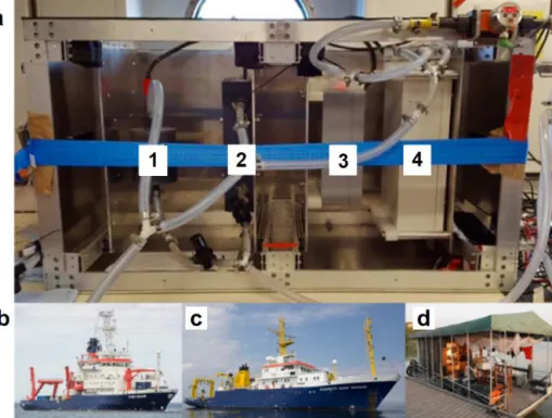
Figure 2.Complete flow-through set-up(a)in operation on board RVMeteor, indicating the easily accessible sensors for O2(1),T andS (2), andpCO2(3) and CH4(4). Besides the operation on RVMeteor, M133,(b)across the Atlantic, the set-up was also deployed on RV Elisabeth Mann Borgese, EMB 142,(c)within the Baltic Sea and on a houseboat in the Danube Delta(d), Romania, for spring (Rom1), summer (Rom2) and autumn (Rom3).
Cape Town, South Africa, to Islas Malvinas, Argentina, be- tween 15 December 2016 and 13 January 2017 (open to shelf oceanic waters). Discrete samples were collected throughout the cruise for total alkalinity (TA), dissolved inorganic car- bon (DIC), CH4and O2. The water was pumped up by means of a submersible pump installed in the ship’s moon pool at about 5.7 m depth. The system logged once every minute, which was deemed sufficient until the Patagonian Shelf was reached, where the measurement frequency was increased to 1 Hz. Sea surface temperature data were measured with a temperature sensor (SBE 38; Sea-Bird Scientific, Belle- vue, WA, USA) installed at the seawater intake in the moon pool, which was used for temperature correction of the flow- through system data. Sea surface salinity was taken from the ship’s thermosalinograph (SBE 21; SeaCAT thermosalino- graph (TSG); Sea-Bird Scientific, Bellevue, WA, USA) lo- cated within the mess room, and the water inlet was located on the bulbous bow. These salinity data were used for the car- bonate system calculations related to the discrete reference.
CH4 data collected during this cruise were not used due to an internal issue of the detector related to absorption peak identification. These data were automatically flagged within the sensor diagnostic values and subsequently excluded. This issue was fixed for the limnic campaigns by the installation of a reference gas cell in the absorption path of the detector.
2.3.2 Elisabeth Mann Borgesecruise EMB 142 to the western Baltic Sea (brackish)
The sensor package was run on board the RVElisabeth Mann Borgese (EMB 142) during a cruise to the western Baltic Sea between 15 and 22 October 2016 (brackish waters). The cruise was one of the main field activities of the Scientific Committee on Oceanic Research (SCOR) working group 142 (under the project titled “Dissolved N2O and CH4measure- ments: Working towards a global network of ocean time se- ries measurements of N2O and CH4”) and was entirely dedi- cated to the inter-comparison of continuous and discrete N2O and CH4measurement techniques (see Wilson et al., 2018), but some of the systems also measuredpCO2continuously.
Discrete samples were collected for validation of the CO2 and CH4sensors. All analysers and the discrete sampling line were connected to the same water supply from a submersible pump system installed in the ship’s moon pool (depth 3 m), ensuring that the same water was used by all groups. A back- pressure regulation system assured the independent flow as- surance of the individual set-ups. The sensors logged contin- uously at a rate of between once per second and once per minute, depending on local variability. During this cruise, only half the CH4data were used due the same technical rea- son as stated for the oceanic cruise.
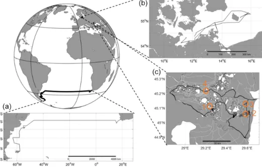
Figure 3.Transects for all test sites.(a)Oceanic – South Atlantic; RVMeteor, cruise M133; ocean (Cape Town, South Africa, to Stanley, Islas Malvinas).(b)Brackish – RVElisabeth Mann Borgese, cruise EMB 142; western Baltic Sea.(c)Limnic – Rom1–3; Danube Delta, Romania. Orange circles, labelled 1 through 4, show the stations of stationary overnight stops (see Fig. 11). For further information, see Table 2.
2.3.3 Romania 1–3 cruises in the Danube river delta, Romania (limnic)
Campaigns over three consecutive seasons were conducted during three field campaigns throughout the Danube Delta in Romania (limnic) in 2017, namely during spring (Rom1 – 17–26 June 2017), summer (Rom2 – 3–12 August 2017) and autumn (Rom3 – 13–23 October 2017). The Danube Delta is situated at the border of Romania and Ukraine on the edge of the Black Sea. It is the second-largest river delta in Europe with a diverse wetland area of about 3000 km2, with a vari- ety of lakes, rivers and channels. The equipment was set up on board a small houseboat, giving access to smaller chan- nels and hard to reach areas. A small power generator or car batteries were used to power the system. With an 11–24 V power source, the set-up can take readings at up to 1 Hz. In combination with the flow-through set-up, discrete samples were collected using the same water inlet as the sensors prior to the sensor inlet, with little disruption to the overall water flow. Data acquisition was only interrupted when there were unexpected rainstorms or problems with the power supply, i.e. power cuts due to lack of fuel. Bilge pumps were de- ployed from the bow of the house boat to reduce water body perturbations caused by the boat that would affect the flow- through measurements. The excess water was discarded over the side, away from the pump location. A few times during the deployment, there were no SBE data since the data log- ging did not automatically restart after a re-powering of the system. During these times, temperature data from the optode
(mean offset from the SBE for all cruises 0.16±0.10◦C) were used instead.
2.4 Method validation
To validate the sensor measurements, discrete samples were collected simultaneously from the same water source (vessel dependent) using tubing connected to the manifold that was connected to the sensors.
TA and DIC samples were collected in 500 mL Duran glass bottles (100 mL borosilicate glass bottles for inland waters) following the standard operating procedure for wa- ter sampling for the parameters of the oceanic carbon diox- ide system (SOP 1; Dickson et al., 2007), with 87, 8 and 68 discrete samples from the oceanic, brackish and inland water cruises, respectively. The samples were poisoned with 100 µL (20 µL inland) of saturated HgCl2 solution to stop biological activity from altering the carbon distributions in the sample container before analysis, a procedure not typ- ically performed in limnic research. A headspace of ap- proximately 1 % of the bottle volume was left to allow for water expansion. A greased stopper was put in place and secured in an airtight manner, using an elastic strap. The samples were then stored in a dark, cool place until mea- sured. The versatile instrument for the determination of titra- tion alkalinity (VINDTA; Marianda Marine Analytics and Data, Kiel, Germany) and single-operator multiparameter metabolic analyser (SOMMA; University of Rhode Island, Narragansett Bay, MA, USA) were used to measure TA (Mintrop et al., 2000) and DIC (Johnson et al., 1987) in
the brackish and seawater samples. Freshwater samples were measured using a total alkalinity titrator (model AS-ALK2;
Apollo SciTech, LLC., Newark, USA) and a DIC analyser (model AS-C3; Apollo SciTech, LLC., Newark, USA). Mea- surements were calibrated with certified reference material (CRM) provided by Andrew Dickson (University of Cali- fornia, San Diego, CA, USA), with a determined precision of ±1.64 and ±1.15 µmol kg−1, respectively, for DIC and TA, and freshwater precision from duplicates was±1.29 and
±2.90 µmol kg−1for DIC and TA, respectively.
TA and DIC were then used to compute pCO2, using the open-access CO2SYS software (Lewis et al., 1998), employing the Millero (2010), Millero et al. (2006) and Millero (1979) carbonic acid dissociation constants (K1 and K2) for seawater, brackish and freshwater samples, respec- tively. For the pH scale and KSO4 dissociation constants, seawater and Dickson and Riley (1979), were used.
CH4 samples were collected in 20 mL bottles, poisoned with 50 µL of saturated solution HgCl2and crimp sealed. The samples were then stored until measurement. CH4in these water samples was measured with a gas chromatographic method, following a procedure described by Weiss and Price (1980) and Annette Kock (unpublished data), with an av- erage standard deviation of the mean CH4concentration of 2.7 % calculated following Annette Kock (unpublished data) and David (1951). During transportation and storage, some CH4samples developed air bubbles due to warming causing some of the gases (e.g. nitrogen and oxygen) to become su- persaturated and eventually outgas; these samples were dis- carded.
During the brackish water cruise, the mobile equilibrator sensor system (MESS; Leibniz Institute for Baltic Sea Re- search) was used as a reference system. The system consists of an open, mixed showerhead bubble-type equilibrator, with an auxiliary equilibrator attached to the main exchange ves- sel. Water flow was adjusted to approximately 6 L min−1dur- ing the cruise. A total of three cavity-enhanced absorption spectrometers (CEAS) were attached in parallel and from which only the results of the greenhouse gas (GHG) anal- yser (Los Gatos Research (LGR), San Jose, CA, USA) de- termining xCO2 andxCH4 were used for comparison pur- poses in this study. Total airflow through the pumps of the sensors, and an additional air pump, was set to approximately 1 L min−1. A set of calibration gas runs covered a range from 1806 to 24 944 ppb for methane and 201.3 to 1001.5 ppm for CO2. The source of the calibration gases was the central cal- ibration facility of the European Integrated Carbon Observa- tion Research Infrastructure (ICOS Central Analytical Labo- ratories – CAL). The high standard was produced by the Na- tional Oceanic and Atmospheric Administration (NOAA) as an initiative of the SCOR working group 143. The response times for methane and CO2for the chosen flow rates were de- termined prior to the cruise to be approximately∼330 and
∼35 s, respectively, at roughly 6 L min−1, with a gas flow of 4.7 L min−1. Similar system operations and details of the
post-processing of the data are given in Gülzow et al. (2011), which is installed on a voluntary observing ship (VOS) line and regularly reports the data to the Surface Ocean CO2AT- las (SOCAT) database (Bakker et al., 2016).
Oxygen was sampled in 100 mL borosilicate glass bot- tles with a precisely known volume and titrated using the Winkler method (Winkler, 1888) on the oceanic cruise. The precision of the Winkler-titrated oxygen measurements was 0.29 µmol L−1and based on 120 duplicates from the mathe- matical average of standard deviations per replicate. Samples containing any air bubbles were discarded.
2.5 Sensor data processing
The corrections on the rawpCO2output from the HC–CO2 sensor were for sensor drift (Sect. 2.5.1; both zero and span), any observed warming of the sampled water at the sensor with respect to the seawater intake temperature (Sect. 2.5.2), extended calibrations (Sect. 2.5.3; over 6000 ppm, i.e. the up- per limit of manufacturer calibration range; although cali- brated with xCO2, the final data by the sensors were con- verted topCO2) and the effect of the sensor response time (RT; Sect. 2.5.4).
2.5.1 Sensor drift
Sensor drift for the HC–CO2 was corrected on the basis of pre- and post-deployment calibrations and the regular in situ zeroings, using the sensor’s auto-zero function, in which CO2is scrubbed from the measured gas stream using a soda lime cartridge. This zero measurement is then used in post- processing to correct for the drift over the deployment, de- tails of which are described in Fietzek et al. (2014). The ze- roings were carried out at regular intervals of 4 to 12 h in the various field campaigns, and for correction during process- ing, we considered the temporal change in the concentration- dependent response of the sensor between pre- and the post- cruise factory calibration, i.e. span drift, to be linear to the sensor’s runtime.
2.5.2 Temperature correction
The temperature correction was applied for allpCO2data to correct for any temperature difference between measurement in the flow-through set-up and in situ temperature. After a time lag correction due to an in situ temperature and equi- librium temperature mismatch resulting from the travelling time of the water from intake to sensor spot (Takahashi et al., 1993), the temperature correction was used forpCO2as follows:
pCO2(Tin situ)=pCO2(Tequ)·exp[0.0423·(Tin situ−Tequ)], (1) where Tin situ is the in situ temperature (i.e. sea surface temperature, SST, from inlet), andTequ is the equilibration temperature. For CH4, the correction, following Gülzow et
al. (2011), was applied as follows:
pCH4=pCH4,equ·
CH4,sol,equ CH4,sol,in situ
, (2)
wherepCH4is the finalpCH4(atmosphere – atm),pCH4,equ is thepCH4(atm) at equilibrium, CH4,sol,equ is the solubil- ity (mol (L atm)−1) of CH4at equilibrium temperature and CH4,sol,insitu is the solubility (mol (L atm)−1) at the in situ temperature.
2.5.3 Extended calibrations
During the Danube river field campaigns, CO2 data some- times exceeded 6000 ppm, i.e. the upper limit of the factory calibration range. NDIR detectors, such as the one used in the HC–CO2 sensor, show a non-linear signal response; there- fore, extrapolation over the factory-calibrated range could not be done safely, and an extended calibration was con- ducted. Prior to the extended calibrations, a further post- processing calibration was conducted by the manufacturer.
The polynomial was compared to that of the initial post cal- ibration from Rom2, revealing an average offset between the two of−0.766±0.94 (±SD) ppm. This proved that the HC–
CO2 had shown little change over the period, ensuring the extended calibration was still applicable and could be ap- plied to this campaign. The extended lab calibration was per- formed on manually produced gas mixtures. The xCO2 of these mixtures was calculated considering the precisely mea- sured flow ratios of the mixed gases N2and CO2. The pre- pared calibration gas was wetted and routed to the HC–CO2 membrane equilibrator. An extended calibration curve was then estimated to reduce the measurement uncertainty over an extended range of 5000–30 000 parts per million by vol- ume (ppmv). Still, the measurement error at this range of ap- proximately 3 % is larger than the±1 % accuracy for mea- surements within the regular factory calibration range. This was due to larger uncertainties in the calibration reference (N2and CO2; Air Liquide, Düsseldorf, Germany; 99.999 % and 99.995 % accuracy, respectively), the flow error of the mass flow controllers and the smaller sensor sensitivities at higher partial pressures. Although calibrated withxCO2, fi- nal data by the sensors were converted topCO2in µatm.
2.5.4 Response time
The HC–CO2sensor response time (RT) for the correspond- ing flow rate and temperature was estimated from the sig- nal recovery after each zeroing interval by fitting an expo- nential function to the signal increase following the zeroing.
Sensor response time is typically denoted ast63, which rep- resents the e-folding timescale of the sensor, i.e. the time over which, following a stepwise change in the measured property, the sensor signal has accommodated 63 % of the step’s amplitude (Miloshevich et al., 2004). This correction was carried out by following a RT correction (RT-Corr) rou- tine by Fiedler et al. (2013). However, the conditions within
the limnic regions were simply too variable compared to the available in situ RT determinations and the in situ RT de- pendencies that could be derived from the in situ measure- ments. Therefore, prior to the first campaigns, experiments were conducted within temperature-controlled culture rooms to see how thee-folding time of the HC–CO2flow-through sensor was affected by flow and temperature. These char- acterizations were used as the basis for the HC–CO2 RT- Corr for the limnic cruises, as described below for HC–CH4. Procedures for RT-Corr are further described by Fiedler et al. (2013) and Miloshevich et al. (2004).
Due to the HC–CH4 using a TDLAS detector, drift cor- rection was not needed as it produces a derivative signal that is directly proportional to CH4, eliminating offsets in a zero baseline technique along with a narrow band detec- tion, therefore reducing signal noise (Werle, 2004). However, compared to the HC–CO2, the HC–CH4 sensor has an ap- proximately 15 times longer RT due multiple combined rea- sons, namely lower solubility, lower CH4permeability of the membrane material and the comparatively larger internal gas volume. To enable a meaningful analysis of all the dissolved gas sensor signals, the CH4data therefore needed a RT-Corr.
This was derived in a different way to the HC–CO2, as no zeroing process within the HC–CH4 allowed regular phe- nomenological estimation of the in situ RT during measur- ing. To quantify the CH4sensor’st63, laboratory experiments with a modified sensor unit were conducted at different flow rates (5.7, 6.5 and 7 L min−1) and temperatures (11.06, 15.05 and 18.04◦C) to determine the RT as a function of these pa- rameters. The HC–CH4 used for the RT determination ex- periments was modified by the installation of two additional valves in the internal gas circuit (see the sensor schematic in the Fietzek et al., 2014). Switching these valves enables the bypassing of the membrane equilibrator and causes, for example, equilibrated, lowpCH4gas to be continuously cir- culated through the detector. Then, thepCH4in the calibra- tion tank could be increased. As soon as a stablepCH4level was reached in the tank, the valves within the HydroC were switched back and the gas passed the membrane equilibrator again. From the resulting signal increase, the time constant for the equilibration process, i.e. the sensor RT, could be de- termined.
These modifications only affected the internal gas volume and flow properties to a small extent. An effect on the de- termined RT, compared to the RT of a standard HC–CH4, is therefore considered negligible. This information was then applied to the raw HC–CH4field data, considering the mea- sured flow rate and temperature and the method of (Fiedler et al., 2013).
Post-processing of the HC–O2followed the SOP provided by KMCON, using Garcia and Gordon (1992) combined fit constants. Further processing to convert the output into gravimetric (µmol kg−1) and volumetric units (µmol L−1) for comparison with other sensors and the discrete sam- ples is described in the SCOR WG142 recommendations on
Figure 4.Calibration polynomial from the post-cruise manufacturer calibration (grey dots; KMCON) and the manual extended calibra- tion curve (black dots), with the top range of the KMCON cali- bration range indicated (dashed line) above which the non-linear behaviour of the non-dispersive infrared (NDIR) spectrometry sen- sor becomes stronger. The processed signal was calculated from the raw and reference signal data during processing.
O2 quantity conversions (Bittig et al., 2018a). During the oceanic cruise, an average offset of−19.04±2.26 (±root mean square error – RMSE) µmol L−1 and−29.78±5.04 (±RMSE) µmol L−1was also found within the open ocean and shelf, respectively, to discrete oxygen data. Two separate linear offset corrections were applied throughout all oceanic data. Significant optode sensor drift, particularly when the sensor is not in the water, is a well-documented phenomenon (Bittig et al., 2018b).
The output from the factory-calibrated SBE 45 thermos- alinograph had no need for post-processing. All accuracies of the sensors are shown in Table 1.
3 Results
The set-up was easily adapted to each power source, manag- ing to measure across the range of salinities and concentra- tions (Table 2). The results of the corrections are shown in the following sections.
3.1 Extended calibration
Compared with the prior calibration curve from the con- ducted calibration at KMCON, the final extended 5◦ poly- nomial had to be shifted slightly (690 ppm). This was ex- pected due to slightly different calibration methods and was done so that both polynomials matched at the top of the cal- ibration range from KMCON (∼6000 ppm). The sensor was able to reach values of nearly 30 000 ppm before starting to reach saturation (Fig. 4). Given that this range was of simi- lar magnitude to discrete samples and previous pCO2 data
from the Danube Delta (Marie-Sophie Maier, unpublished data; reaching values of up to and over 20 000 ppm), the cor- rection was applied to all data above 6000 ppm. However, note that the general uncertainty of the sensor at this range is larger than that at company operational values, and due to the longer time period between deployments, spring and summer campaigns have an unquantified increased error. We assume 3 % as a conservative estimate of the overall accuracy of the xCO2 measurements in the extended range (>6000 ppm).
From the noise of the signal during the calibrations, the es- timated precision is±1 % of the CO2reading, and we think that, even at this reduced accuracy, the observations in the highpCO2range are of significant scientific value.
3.2 RT correction analysis
The HC–CO2response time correction (RT-Corr) laboratory experiments quantitatively show the effect of temperature and flow and point to the importance of recording the flow data (Fig. 5). As stated before, due to varying flow and tem- perature, the HC–CO2RT was determined by the laboratory experiments shown in Fig. 5a. An example of the estimation oft63is given in Fig. 5b, which shows the signal recovery fol- lowing a zeroing procedure, witht63=93 s. Both increased flow rate and temperature reduce the RT of the sensor signif- icantly.
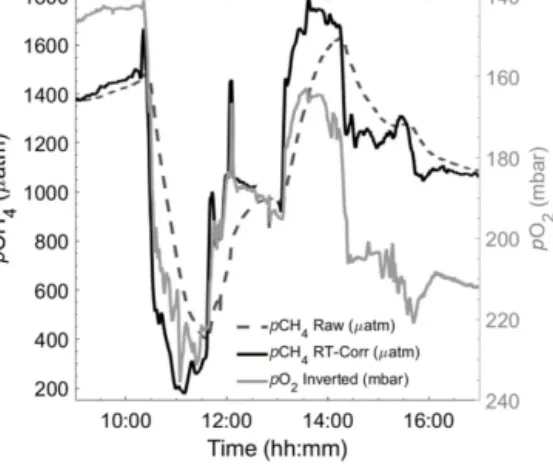
The RT of the HC–CH4was far higher than for CO2and varied between 1425 and 1980 s (Fig. 5c), depending on tem- perature and flow, with both higher temperature and flow rate yielding shorter RT (for comparison,t90for the HC–CO2and HC–CH4was 212 and 3145 s, respectively). This was then applied to the raw HC–CH4data and compared with thepO2, which has a RT of<3 s (KMCON; HydroFlash user manual) and therefore does not require an RT correction, to qualita- tively assess the suitability of the correction, which can be seen from the near-perfect qualitative match betweenpCH4 andpO2(Fig. 6). Note the invertedpO2due to typically hav- ing an inverse relationship withpCH4.
3.3 Verification by discrete sample comparison 3.3.1 CO2
Discrete pCO2 was calculated from TA and DIC mea- surements that had an average precision from replicates of 1.48 µmol kg−1(TA) and 1.04 µmol kg−1(DIC) after the re- moval of one outlier sample. During the oceanic cruise, this provided a mean difference within the open ocean of−0.13±
5.25 µatm (±SD) to the data measured by the HC–CO2flow- through system (HC–CO2 pCO2 – calculatedpCO2; DIC and TA). This mean increased within the productive waters along the Patagonia Shelf to up to 2.56±6.21 µatm (±SD).
A comparison between the performances of the HC–CO2 is shown in Fig. 7, where each region has been separated.
The comparison for the brackish water is against the cali-
Figure 5.Response time (s) of the HC–CO2determined at four temperatures within controlled laboratory conditions for different water flow rates (2, 5 and 8 L min−1) with errors too small to see(a). An example of the output(b)shows howt63is retrieved after a zeroing interval, witht63determined by the model’s fit (line in red). Response time (RT) forpCH4is also shown(c)for flow rates of 5.7, 6.5 and 7 L min−1 conducted in controlled conditions at KMCON.
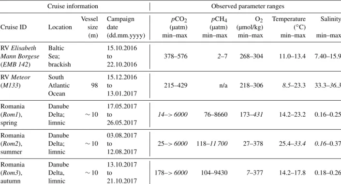
Table 2.Cruise table for all field campaigns in 2016 and 2017, with cruise/ship names (cruise ID in italic), areas and observed maximum to minimum values for all measured parameters (in italic). ForpCO2, the sensor is only factory calibrated up to 6000 ppm; therefore, this was deemed as being the maximum in these circumstances.
Cruise information Observed parameter ranges
Vessel Campaign pCO2 pCH4 O2 Temperature Salinity
Cruise ID Location size date (µatm) (µatm) (µmol/kg) (◦C)
(m) (dd.mm.yyyy) min–max min–max min–max min–max min–max
RVElisabeth Baltic 15.10.2016
Mann Borgese Sea; to 378–576 2–7 268–304 11.0–13.4 7.40–15.9
(EMB 142) brackish 22.10.2016
RVMeteor South 15.12.2016
(M133) Atlantic 98 to 215–429 n/a 218–306 8.5–23.3 33.3–36.3
Ocean 13.01.2017
Romania Danube 17.05.2017
(Rom1), Delta; ∼10 to 14–>6000 76–8660 173–431 14.2–23.2 0.16–0.25
spring limnic 26.05.2017
Romania Danube 03.08.2017
(Rom2), Delta; ∼10 to 25–>6000 118–11 700 27–378 25.4–33.4 0.16–0.37
summer limnic 12.08.2017
Romania Danube 13.10.2017
(Rom3), Delta, ∼10 to 178–>6000 104–9430 7–377 14.2–17.8 0.18–0.26
autumn limnic 21.10.2017
n/a: not applicable.
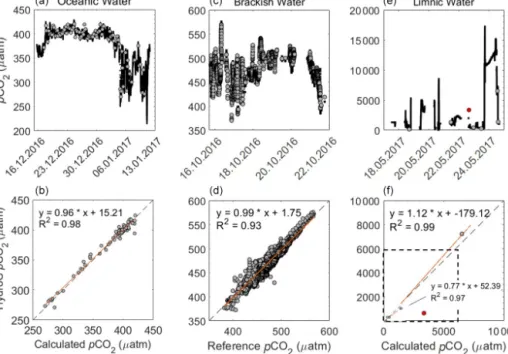
brated data from the state-of-the-art equilibrator set-up, us- ing an LGR off-axis ICOS (Gülzow et al., 2011) showing an offset of−2.87±7.71 (±SD) µatm (HC–CO2– reference pCO2). Note the change in pCO2 for each region, varying from undersaturated (mainly oceanic waters) to supersatu- rated (brackish waters) and almost 20 000 µatm within the limnic waters during Rom1 (Fig. 7).
The limnic measurements of TA and DIC had an average precision based on replicates of 1.03 and 0.27 µmol kg−1for TA and DIC, respectively.
3.3.2 CH4
The average offset of the reference system to the HC–CH4
during the first half of the brackish cruise was−0.95±0.19 (±SD) µatm for the RT-CorrpCH4data (Fig. 8). This gave an average offset within the manufacturer accuracy specifi- cation range of±2 µatm, with a mean offset of 0.79±0.64 (±SD) µatm. Both sensors showed the same variability and magnitude to one another, even with the offset (Fig. 8).
Given the previous evaluation of the RT-Corr, this im- proved the accuracy of the HC–CH4 within the limnic sys- tem of Romania (HC–CH4– measuredpCH4; Rom1 – from
Figure 6. Section of a 24 h cycle of data from the autumn limnic cruise (Rom3), showing raw (black dashed line) and RT-Corr (black solid line)pCH4µatm measured by the HC–CH4with invertedpO2 mbar (grey line) as a technically independent, yet parameter-wise, linked reference for real-time spatiotemporal variability, i.e. RT O2 sensorRT CH4sensor.
−164.3±1117.3 (±SD) µatm to 182.6±591.3 (±SD) µatm;
Rom2 – from 609.3±1065 (±SD) µatm to 537.9±1145 (±SD) µatm; Rom3 – from 466.5±383 (±SD) µatm to 457.1±376 (±SD) µatm; Rom1 is shown in Fig. 9). Match- ing discrete sample data with continuous sensor data that have a long RT becomes very complicated in highly vari- able situations. The effect of variable situations was also no- ticeable within the triplicates of the discrete samples, with some varying by over 400 µatm (with an average variabil- ity between repeated samples at 122.6±100.9 (±SD) µatm), leading to the offset with the HC–CH4seeming reasonable.
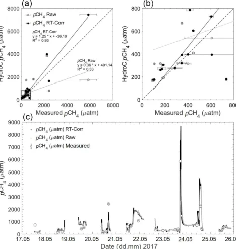
The agreement between sensor data and discrete samples in- creased significantly with the RT-Corr, as shown in Fig. 9, with theR2improving from 0.33 to 0.93 and the slope from 0.36 to 1.25. Peaks within the data are also observed within the discrete measurements (Fig. 9c) in combination with the sensor data, e.g. Fig. 9c between 20.05 and 21.05. It has to be noted that the determination of dissolved CH4concentrations from discrete samples is also not fully mature and shows significant inter-laboratory offsets (Wilson et al., 2018), and thus, the observed discrepancy is likely not to be entirely caused by our sensor-based measurements.
3.3.3 O2
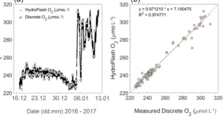
During the oceanic cruise, after the post-offset correc- tion (stated above), O2µmol L−1 had an average offset of
−0.1±3.4 (±SD) µmol L−1 (HydroFlash O2 – discrete samples O2) over the whole transect (Fig. 10). Although sta- ble and matching the variability throughout (Fig. 10a), note the increased offset observed when entering the Patagonian Shelf (Fig. 10b).
4 Discussion
We have presented a portable, easily accessible, quick to set up multi-gas measurement system that can autonomously measure across the entire LOAC. The operational boundaries of these sensors were tested over various deployment dura- tions (∼1 month to hours), small spatial scales and under a wide range of operational environmental conditions.
OceanicpCO2sensors are needed to operate with an over- all accuracy of±2 µatm (Pierrot et al., 2009); therefore, this sensor performance throughout the open ocean was consid- ered to be very good (Sect. 3.3.1). The offset found during the oceanic campaign, when entering the Patagonian Shelf (5.26±4.33 µatm), is potentially due to biofouling within the tubing from the pump to the sensors. The offset observed by the optode for O2increased during the Patagonian Shelf waters due to the higher concentration ranges and gradients found along the shelf, possibly indicating an emerging bio- fouling issue of the sensor or within the casing surrounding the sensor. This demonstrated the overall relatively long-term stability and reliability of the O2optode even in an area with such extreme hydrographic variability. This was expected due to optodes being used widely in multiple environments (see Bittig et al., 2018b, Kokic et al., 2016, and Wikner et al., 2013, for oceanic, coastal and fresh water examples).
In the brackish water campaign, the HC–CO2 and HC–
CH4 showed good agreement with the reference systems within the manufacturer’s specifications. The data from the HC–CH4, although having an internal issue as stated in Sect. 2.3.1, showed the same magnitude and variability as the reference system (Fig. 8). With little noise from both sys- tems, natural variability was witnessed by both to further as- sure us that the system was running efficiently.
The limnic campaigns were ideally suited to test the flex- ibility of these sensors, with concentration ranges reaching almost 30 000 µatm forpCO2, over 10 000 µatm forpCH4 and O2ranging from supersaturated to suboxic. Direct com- parisons with the CH4 and CO2 concentrations show rela- tively similar variations to previous measurements within the Danube Delta lakes (Durisch-Kaiser et al., 2008; Pavel et al., 2009). Due to the design, physical placement and high flow speed, no biofouling of the membranes of the HC–CO2and HC–CH4 occurred even within particle-rich environments, with very little settlement during our campaigns. However, our campaigns consisted of continuous movement through varying regions, and therefore, long-term stationary deploy- ment in highly particulate waters may potentially lead to set- tlement. Overall, the set-up showed a good performance with continuous data collection, providing values within the ex- pected ranges forpCO2 across different salinity areas and when split into lakes rivers and channels (Hope et al., 1996;
Bouillon et al., 2007; Lynch et al., 2010). However, in com- parison to rivers and streams of a similar size,pCH4 deter- mined in this study generally had higher overall concentra- tions (Wang et al., 2009; Crawford et al., 2017) and higher
Figure 7.pCO2(µatm) from the HC–CO2within the following three regions: oceanic (aandb, including the open ocean and the Patagonian Shelf), brackish(c, d)and limnic waters(e, f)with the reference data used. The top graphs show the overall transects, with HC–CO2data as a black line and the reference data as grey dots (date presented as dd.mm.yyyy). The lower graphs are property–property plots showing the 1:1 line (dashed) and the line of the best linear fit (orange). For the validation of our system, we used the calculatedpCO2from TA and DIC, using CO2SYS for both oceanic and limnic waters, whereas a reference system was used for the brackish waters, as described above.
During the Rom1 (limnic cruise),n=7 with the outlier in red (sample with an unclear match to flow-through data excluded from fit), with the box (dashed line) indicating the 6000 ppm company calibration limit.
Figure 8.pCH4µatm data from the HC–CH4during the brackish cruise (EMB 142; RVElisabeth Mann Borgese) expedition in the western Baltic Sea, with the reference system over the first half of the cruise. Panel (a)shows the HC–CH4 data with a negative offset, resulting in lower concentrations compared to that of the reference data. Panel(b)shows a 1:1 plot, with a regression line (R2=0.928) illustrating the constant offset, but with a similar slope of data. Within the brackish waters, the offset was within the spec- ifications from KMCON, yet both values (reference and HC–CH4) were in the range of that previously found within the region (Gül- zow et al., 2013).
overall medians (Stanley et al., 2016). Yet, they are within the range found for other freshwater systems and on a simi- lar scale with other regions, showing large increases in CH4
concentrations (Bange et al., 2019). When focusing on the discrete sample comparison between the calculated pCO2
(from TA and DIC) and measuredpCO2 (HC–CO2) in the limnic cruise (Sect. 3.3.1), the deviation was not unexpected due to the likely presence of organic alkalinity that causes an unknown TA bias leading to an offset in the calculatedpCO2 (Abril et al., 2015).
Having the combination of all these sensors, especially with CH4, makes this set-up more unique for measurements across the LOAC. Due to the high accuracy needed for oceanicpCO2 measurements, optimization and continuous improvements of these measurements has been occurring for decades (Körtzinger et al., 1996; Dickson et al., 2007; Pier- rot et al., 2009) yet for a comparatively narrow range of oceanic conditions. Sensors have undergone multiple devel- opments and improvements over these years, with the fo- cus on measurements within these water bodies with high accuracy for a relatively small concentration range. In the market, there are currently few oceanicpCO2sensors capa- ble of measuring under environmental conditions that cross the boundaries from limnic to oceanic, including the SAMI- CO2 ocean CO2sensor (Sunburst Sensors, LLC, Missoula, MT, USA; see DeGranpre et al., 1995; Baehr and DeGrand-
Figure 9. (a) Rom1pCH4µatm data versus measured discrete samples ofpCH4µatm, with both raw HC–CH4data and response time corrected (RT-Corr) data over the full range of concentrations.(b)A close-up view of the lower 800 µatm, with errors for the measured samples against the HC–CH4data. The grey line signals the line of best fit for the raw pCH4, and the black line signals the RT-Corr pCH4µatm.(c)The full transect with discretepCH4µatm samples for the spring cruise over time (date in dd.mm), but some error bars are too small to see.
pre, 2004; and Phillips et al., 2015). However, with simi- lar accuracies in the ocean, one advantage of the continu- ous NDIR/TDLAS-based instruments used here is that no chemical consumables are required for the measurements (refer to the review papers for a discussion of different sen- sors, i.e. Clarke et al., 2017, and Martz et al., 2015, and for current technological updates on carbonate chemistry instru- mentation, refer to the International Ocean Carbon Coordi- nation Project, IOCCP, at http://www.ioccp.org/, last access:
30 October 2020). Traditional flow-through systems, on the other hand, such as the commonly used GO system (Gen- eral Oceanics, Miami, FL, USA), are generally larger, more complex and built from more components. They also require more maintenance (see reference gases), and the data ac- quisition is therefore more labour-intensive, also increasing the probability of human error. Sensors designed for inland water bodies tend to be on the lower price range for vari- ous reasons, which unfortunately leads to lower accuracies and greater inconsistencies (Meinson et al., 2016; Friedling- stein et al., 2019; Canning, 2020). Measurements across the
LOAC need high-accuracy sensors as the concentrations and dynamic ranges usually decrease from inland waters to the ocean and, thus, have to match with the oceanic standards, and the set-up presented here was designed to fulfil these re- quirements.
Due to the higher quantity and quality of temporal and spa- tial measurements needed (Natchimuthu et al., 2017), below we present data examples from our various field campaigns to illustrate the utility and observational power of our ap- proach to resolving both spatial and temporal variability in parallel for all measured quantities and at a very high resolu- tion.
4.1 Temporal variability
In the Danube Delta, the portability of the set-up allowed us to focus on temporal variability for specific regions over three seasons. Due to the low power consumption, the small generator and car batteries were sufficient to easily run the entire set-up, allowing for high-resolution (up to 1 Hz), con-
Figure 10.Oxygen concentration during cruise M133 from recal- ibrated continuous optode and discrete Winkler titration measure- ments(a)and a property–property plot(b). For the open ocean and shelf waters, the mean offset is−0.08±1.89 (±SD) µmol L−1and
−0.15±6.49 (±SD) µmol L−1, respectively. Higher variability to- wards the end of the transect is due to entering the productive Patag- onian Shelf (06.01.2017–13.01.2017), which is also seen in higher concentrations of O2.
tinuous measurements to extract diel cycles in the same way over the three seasons. Figure 11 displays data from a 2-week field campaign (Rom3), with areas of stationary measure- ments over extended time periods (grey shading in Fig. 11;
see Fig. 3c for locations). Data were continuously logged for all parameters throughout the campaigns, with interruptions only when the houseboat docked. During each campaign, temporal variability showed differences between the regions (lakes, rivers and channels). The stationary phase of the first campaign was in a channel next to Lake Isaac (Fig. 11; grey box on 16.10.; duration 15 h:26 min; Fig. 3c1). An instant peak in CO2and CH4can be seen when entering the channel from the lake, coinciding with a drop in O2. Over this diel cycle, CO2 and O2 are apparently governed by production and respiration, as expected (Nimick et al., 2011), yet with relatively constant and high CH4 concentrations. However, during the second stationary zone measurements (Figs. 11;
3c2; 19.10.) conducted within a lake,pCO2is shown to in- crease steadily during the station, while always remaining far lower than within the channel. The same diel pattern is shown in the final station’s stationary phase (Figs. 11; 3c4; 23.10.), which is located in one of the northern channels, far from any lake. These comparisons (from channel to lake variabili- ties) throughout the transects show the temporal variabilities within regions adjacent to, or within close proximity to, one another and differ vastly in both magnitude and diel pattern, even when comparing the same region (channel next to a lake – 16.10.; a further northern channel – 23.10.; Figs. 11; 3c4).
Looking closer into specific temporal variabilities, Fig. 12 shows an exemplary 24 h cycle within a small channel. This location was marked as a hotspot within our transect, show- ing drastic concentration changes with clear coupling be- tween O2,pCO2and temperature. ThepCO2increases from 5000 µatm to nearly 17 000 µatm during the night, then de-
creases back to initial levels during the day, coinciding with sunrise and sunset, while the opposite trend for both tem- perature and pO2 was observed. Timing and amplitude of these diel trends could have been lost with discrete sampling alone. Due to the same diel variation observed from this lo- cation over 2 of the 3 months (Rom1–2), uncertainties be- hind this variation, such as passing of water parcels anoma- lies or wind-driven variation as suggested before (Serra and Colomer, 2007; Van de Bogert et al., 2012), can be ruled out as possible explanations. Although diel cycles in inland wa- ters have been investigated (for channels, estuarine, lakes and pond investigations, respectively; see Nimick et al., 2011;
Maher et al., 2015; Andersen et al., 2017; van Bergen et al., 2019; Canning et al., 2020b), they are generally left out when it comes to average concentrations and corresponding fluxes. Evaluating our data gives evidence that such practices have to be critically evaluated, especially given the abun- dance and magnitude of diel cycles observed in these regions.
Furthermore, allowing for multiple gases to be measured si- multaneously enables extreme observations, such as this, to shed some light on the processes involved (Canning et al., 2020b). Therefore, any study aiming to measure representa- tive concentrations and fluxes for limnic systems with signif- icant diel variability will have to address this. Adequate sam- pling/observation schemes should be implemented to avoid strong biases (e.g. by both day–night sampling or by convo- luting spatial and temporal variability in 24 h non-stationary mapping exercises).
4.2 Spatial variability
During the limnic campaigns, CH4 showed extreme spa- tial and temporal differences, which highlight the need for high spatiotempral coverage. Although RT-Corr is not a new method within the ocean/brackish waters (see e.g. Fiedler et al., 2013; Gülzow et al., 2011; Miloshevich et al., 2004), the results of both the HC–CO2and HC–CH4corrections show high promise and an absolute need for such sensors in fresh- waters that measure in highly spatially diverse regions. Both system stability and sensitivity could be demonstrated dur- ing the oceanic cruise (15 December 2016–13 January 2017;
Fig. 13). A little spatial variability was expected over the large distance when crossing the open ocean waters of the South Atlantic Gyre. The fact that even these small varia- tions in pCO2, O2 and temperature still show clear corre- lations points at the very low noise level of the measure- ments. The Brazil and Malvinas currents merge when en- tering the Patagonian Shelf, creating upwelling with fresh nutrients and, therefore, strongly increased primary produc- tion (Matano et al., 2010). These waters are characterized by high productivity with higherpO2and lowerpCO2(Fig. 13) and increased overall variability compared to the open ocean.
Some of these variabilities show the dynamic mixing be- tween the contrasting water masses of the confluent surface currents. This region is one of the most productive and en-
Figure 11.Sections acquired during the autumn limnic cruise. Rom3, showingpCO2(µatm; logarithmic scale),pCH4(µatm; logarithmic scale) andpO2(in mbar) and temperature (in◦C; grey) from the SBE across the entire deployment. Temperature is kept constant on the right yaxis for direct changes to be noticed within each gas. Shaded areas and numbers (1–4) indicate periods of stationary observations when anchored in one location (see Fig. 3c1–4), with the station keeping durations in hours and minutes (shown in the middle row). Gaps in data collection refer to times when the systems were switched off.
Figure 12. (a)Measurements ofpCO2(in µatm; blue),pO2(in mbar; orange) and temperature (in◦C; black), during the Danube river campaign, Rom2, in summer 2017. The grey rectangle highlights a 24 h cycle acquired at a fixed location in a channel.(b)Close up of this 24 h cycle, with sunset (solid red) and sunrise (dashed line red) indicated, showing extreme variability in the diel cycle timescale.(c)Cruise track of the campaign, with the red dot indicating the position of the 24 h stationary data acquisition.