arXiv:1108.0501v1 [astro-ph.CO] 2 Aug 2011
M. Ackermann
2, M. Ajello
2, A. Allafort
2, E. Angelakis
3, M. Axelsson
4,5,6, L. Baldini
7, J. Ballet
8,
3
G. Barbiellini
9,10, D. Bastieri
11,12, R. Bellazzini
7, B. Berenji
2, R. D. Blandford
2, E. D. Bloom
2,
4
E. Bonamente
13,14, A. W. Borgland
2, A. Bouvier
15, J. Bregeon
7, A. Brez
7, M. Brigida
16,17,
5
P. Bruel
18, R. Buehler
2, S. Buson
11,12, G. A. Caliandro
19, R. A. Cameron
2, A. Cannon
20,21,
6
P. A. Caraveo
22, J. M. Casandjian
8, E. Cavazzuti
23, C. Cecchi
13,14, E. Charles
2, A. Chekhtman
24,
7
C. C. Cheung
25, S. Ciprini
14, R. Claus
2, J. Cohen-Tanugi
26, S. Cutini
23, F. de Palma
16,17,
8
C. D. Dermer
27, E. do Couto e Silva
2, P. S. Drell
2, R. Dubois
2, D. Dumora
28, L. Escande
28,29,
9
C. Favuzzi
16,17, S. J. Fegan
18, W. B. Focke
2, P. Fortin
18, M. Frailis
30,31, L. Fuhrmann
3,
10
Y. Fukazawa
32, P. Fusco
16,17, F. Gargano
17, D. Gasparrini
23, N. Gehrels
20, N. Giglietto
16,17,
11
P. Giommi
23, F. Giordano
16,17, M. Giroletti
33,1, T. Glanzman
2, G. Godfrey
2, P. Grandi
34,
12
I. A. Grenier
8, S. Guiriec
35, D. Hadasch
19, M. Hayashida
2, E. Hays
20, S. E. Healey
2,
13
G. J´ ohannesson
36, A. S. Johnson
2, T. Kamae
2, H. Katagiri
32, J. Kataoka
37, J. Kn¨ odlseder
38,
14
M. Kuss
7, J. Lande
2, S.-H. Lee
2, F. Longo
9,10, F. Loparco
16,17, B. Lott
28, M. N. Lovellette
27,
15
P. Lubrano
13,14, A. Makeev
24, W. Max-Moerbeck
39, M. N. Mazziotta
17, J. E. McEnery
20,40,
16
J. Mehault
26, P. F. Michelson
2, T. Mizuno
32, C. Monte
16,17, M. E. Monzani
2, A. Morselli
41,
17
I. V. Moskalenko
2, S. Murgia
2, M. Naumann-Godo
8, S. Nishino
32, P. L. Nolan
2, J. P. Norris
42,
18
E. Nuss
26, T. Ohsugi
43, A. Okumura
44, N. Omodei
2, E. Orlando
45,2, J. F. Ormes
42, M. Ozaki
44,
19
D. Paneque
46,2, V. Pavlidou
39,1, V. Pelassa
26, M. Pepe
13,14, M. Pesce-Rollins
7, M. Pierbattista
8,
20
F. Piron
26, T. A. Porter
2, S. Rain`o
16,17, M. Razzano
7, A. Readhead
39, A. Reimer
47,2,1,
21
O. Reimer
47,2, J. L. Richards
39, R. W. Romani
2, H. F.-W. Sadrozinski
15, J. D. Scargle
48,
22
C. Sgr` o
7, E. J. Siskind
49, P. D. Smith
50, G. Spandre
7, P. Spinelli
16,17, M. S. Strickman
27,
23
D. J. Suson
51, H. Takahashi
43, T. Tanaka
2, G. B. Taylor
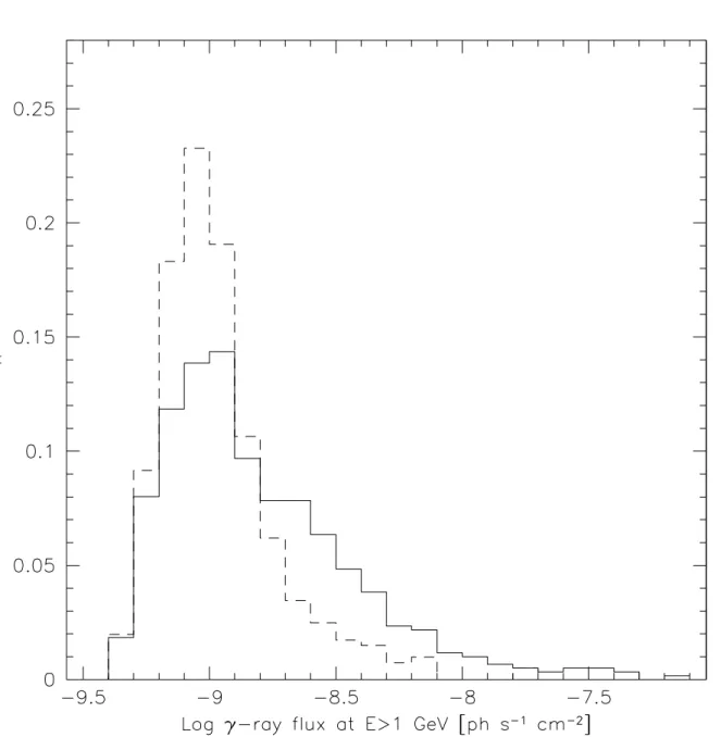
52, J. G. Thayer
2, J. B. Thayer
2,
24
D. J. Thompson
20, D. F. Torres
19,53, G. Tosti
13,14, A. Tramacere
2,54,55, E. Troja
20,56,
25
J. Vandenbroucke
2, G. Vianello
2,54, V. Vitale
41,57, A. P. Waite
2, P. Wang
2, B. L. Winer
50,
26
K. S. Wood
27, Z. Yang
58,6, M. Ziegler
1527
1Corresponding authors: M. Giroletti, giroletti@ira.inaf.it; V. Pavlidou, pavlidou@astro.caltech.edu; A. Reimer, afr@slac.stanford.edu.
2W. W. Hansen Experimental Physics Laboratory, Kavli Institute for Particle Astrophysics and Cosmology, De- partment of Physics and SLAC National Accelerator Laboratory, Stanford University, Stanford, CA 94305, USA
3Max-Planck-Institut f¨ur Radioastronomie, Auf dem H¨ugel 69, 53121 Bonn, Germany
4Department of Astronomy, Stockholm University, SE-106 91 Stockholm, Sweden
5Lund Observatory, SE-221 00 Lund, Sweden
6The Oskar Klein Centre for Cosmoparticle Physics, AlbaNova, SE-106 91 Stockholm, Sweden
7Istituto Nazionale di Fisica Nucleare, Sezione di Pisa, I-56127 Pisa, Italy
8Laboratoire AIM, CEA-IRFU/CNRS/Universit´e Paris Diderot, Service d’Astrophysique, CEA Saclay, 91191 Gif sur Yvette, France
9Istituto Nazionale di Fisica Nucleare, Sezione di Trieste, I-34127 Trieste, Italy
10Dipartimento di Fisica, Universit`a di Trieste, I-34127 Trieste, Italy
11Istituto Nazionale di Fisica Nucleare, Sezione di Padova, I-35131 Padova, Italy
12Dipartimento di Fisica “G. Galilei”, Universit`a di Padova, I-35131 Padova, Italy
13Istituto Nazionale di Fisica Nucleare, Sezione di Perugia, I-06123 Perugia, Italy
14Dipartimento di Fisica, Universit`a degli Studi di Perugia, I-06123 Perugia, Italy
15Santa Cruz Institute for Particle Physics, Department of Physics and Department of Astronomy and Astrophysics, University of California at Santa Cruz, Santa Cruz, CA 95064, USA
16Dipartimento di Fisica “M. Merlin” dell’Universit`a e del Politecnico di Bari, I-70126 Bari, Italy
17Istituto Nazionale di Fisica Nucleare, Sezione di Bari, 70126 Bari, Italy
18Laboratoire Leprince-Ringuet, ´Ecole polytechnique, CNRS/IN2P3, Palaiseau, France
19Institut de Ciencies de l’Espai (IEEC-CSIC), Campus UAB, 08193 Barcelona, Spain
20NASA Goddard Space Flight Center, Greenbelt, MD 20771, USA
21University College Dublin, Belfield, Dublin 4, Ireland
22INAF-Istituto di Astrofisica Spaziale e Fisica Cosmica, I-20133 Milano, Italy
23Agenzia Spaziale Italiana (ASI) Science Data Center, I-00044 Frascati (Roma), Italy
24College of Science, George Mason University, Fairfax, VA 22030, resident at Naval Research Laboratory, Wash- ington, DC 20375, USA
25National Research Council Research Associate, National Academy of Sciences, Washington, DC 20001, resident at Naval Research Laboratory, Washington, DC 20375, USA
26Laboratoire de Physique Th´eorique et Astroparticules, Universit´e Montpellier 2, CNRS/IN2P3, Montpellier, France
27Space Science Division, Naval Research Laboratory, Washington, DC 20375, USA
28Universit´e Bordeaux 1, CNRS/IN2p3, Centre d’´Etudes Nucl´eaires de Bordeaux Gradignan, 33175 Gradignan,
France
29CNRS/IN2P3, Centre d’´Etudes Nucl´eaires Bordeaux Gradignan, UMR 5797, Gradignan, 33175, France
30Dipartimento di Fisica, Universit`a di Udine and Istituto Nazionale di Fisica Nucleare, Sezione di Trieste, Gruppo Collegato di Udine, I-33100 Udine, Italy
31Osservatorio Astronomico di Trieste, Istituto Nazionale di Astrofisica, I-34143 Trieste, Italy
32Department of Physical Sciences, Hiroshima University, Higashi-Hiroshima, Hiroshima 739-8526, Japan
33INAF Istituto di Radioastronomia, 40129 Bologna, Italy
34INAF-IASF Bologna, 40129 Bologna, Italy
35Center for Space Plasma and Aeronomic Research (CSPAR), University of Alabama in Huntsville, Huntsville, AL 35899, USA
36Science Institute, University of Iceland, IS-107 Reykjavik, Iceland
37Research Institute for Science and Engineering, Waseda University, 3-4-1, Okubo, Shinjuku, Tokyo, 169-8555 Japan
38Centre d’´Etude Spatiale des Rayonnements, CNRS/UPS, BP 44346, F-30128 Toulouse Cedex 4, France
39Cahill Center for Astronomy and Astrophysics, California Institute of Technology, Pasadena, CA 91125, USA
40Department of Physics and Department of Astronomy, University of Maryland, College Park, MD 20742, USA
41Istituto Nazionale di Fisica Nucleare, Sezione di Roma “Tor Vergata”, I-00133 Roma, Italy
42Department of Physics and Astronomy, University of Denver, Denver, CO 80208, USA
43Hiroshima Astrophysical Science Center, Hiroshima University, Higashi-Hiroshima, Hiroshima 739-8526, Japan
44Institute of Space and Astronautical Science, JAXA, 3-1-1 Yoshinodai, Chuo-ku, Sagamihara, Kanagawa 252- 5210, Japan
45Max-Planck Institut f¨ur extraterrestrische Physik, 85748 Garching, Germany
46Max-Planck-Institut f¨ur Physik, D-80805 M¨unchen, Germany
47Institut f¨ur Astro- und Teilchenphysik and Institut f¨ur Theoretische Physik, Leopold-Franzens-Universit¨at Inns- bruck, A-6020 Innsbruck, Austria
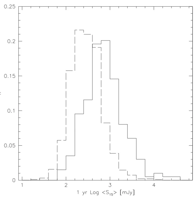
48Space Sciences Division, NASA Ames Research Center, Moffett Field, CA 94035-1000, USA
49NYCB Real-Time Computing Inc., Lattingtown, NY 11560-1025, USA
50Department of Physics, Center for Cosmology and Astro-Particle Physics, The Ohio State University, Columbus, OH 43210, USA
51Department of Chemistry and Physics, Purdue University Calumet, Hammond, IN 46323-2094, USA
52University of New Mexico, MSC07 4220, Albuquerque, NM 87131, USA
53Instituci´o Catalana de Recerca i Estudis Avan¸cats (ICREA), Barcelona, Spain
54Consorzio Interuniversitario per la Fisica Spaziale (CIFS), I-10133 Torino, Italy
55INTEGRAL Science Data Centre, CH-1290 Versoix, Switzerland
56NASA Postdoctoral Program Fellow, USA
ABSTRACT
28
29
We present a detailed statistical analysis of the correlation between radio and gamma-ray emission of the Active Galactic Nuclei (AGN) detected by
Fermiduring its first year of operation, with the largest datasets ever used for this purpose. We use both archival interferometric 8.4 GHz data (from the VLA and ATCA, for the full sam- ple of 599 sources) and concurrent single-dish 15 GHz measurements from the Owens Valley Radio Observatory (OVRO, for a sub sample of 199 objects). Our unprecedent- edly large sample permits us to assess with high accuracy the statistical significance of the correlation, using a surrogate-data method designed to simultaneously account for common-distance bias and the effect of a limited dynamical range in the observed quantities. We find that the statistical significance of a positive correlation between the cm radio and the broad band (E > 100 MeV) gamma-ray energy flux is very high for the whole AGN sample, with a probability
<10
−7for the correlation appearing by chance. Using the OVRO data, we find that concurrent data improve the significance of the correlation from 1.6
×10
−6to 9.0
×10
−8. Our large sample size allows us to study the dependence of correlation strength and significance on specific source types and gamma-ray energy band. We find that the correlation is very significant (chance probability
<10
−7) for both FSRQs and BL Lacs separately; a dependence of the corre- lation strength on the considered gamma-ray energy band is also present, but additional data will be necessary to constrain its significance.
Subject headings:
Gamma rays: galaxies – Radio continuum: galaxies – Galaxies: active
30
– Galaxies: jets – BL Lacertae objects: general – quasars: general
31
1. Introduction
32
After more than 1 year of scanning the gamma-ray sky by the Large Area Telescope (LAT)
33
onboard the
Fermi Gamma-ray Space Telescope (Fermi), the most extreme class of Active Galac-34
tic Nuclei (AGN), blazars (used to refer collectively to BL Lac objects, hereafter BL Lacs, and
35
flat spectrum radio quasars, hereafter FSRQs), remain among the most numerous gamma-ray
36
source populations. Indeed, the First
Fermi-LAT catalog of gamma-ray sources (hereafter 1FGL,37
Abdo et al. 2010a) includes more than 1400 sources and about half of them are believed to be AGNs
38
(Abdo et al. 2010d) with most of them identified via radio catalogs (e.g., CRATES; Healey et al.
39
2007). More than 370 high-latitude (
|b|>10
◦) sources in the 1FGL remain unidentified.
40
57Dipartimento di Fisica, Universit`a di Roma “Tor Vergata”, I-00133 Roma, Italy
58Department of Physics, Stockholm University, AlbaNova, SE-106 91 Stockholm, Sweden
Blazars have been observed to emit at all energies, from the radio band up to very-high energy
41
gamma-rays. Many of the gamma-ray blazars detected so far appear to emit the bulk of their
42
total radiative output at gamma-ray energies. Strong variability across the whole electromagnetic
43
spectrum and on various time scales is considered as one of the most intriguing properties of this
44
source type. In particular their high-energy emission can easily vary by more than an order of
45
magnitude from one observing epoch to the next (e.g. Mukherjee et al. 1997; Abdo et al. 2010c),
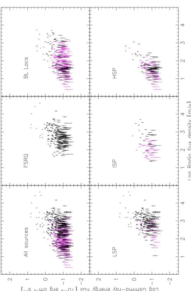
46
and variability time scales at high energies are mostly much shorter (even down to just a few
47
minutes in the TeV band, e.g. Aharonian et al. 2007) than in the long wavelength bands.
48
The high inferred bolometric luminosities, rapid variability, and apparent superluminal motions
49
observed from a range of blazars provide compelling evidence that the non-thermal emission of
50
blazars originates from a region which is propagating relativistically along a jet directed at a small
51
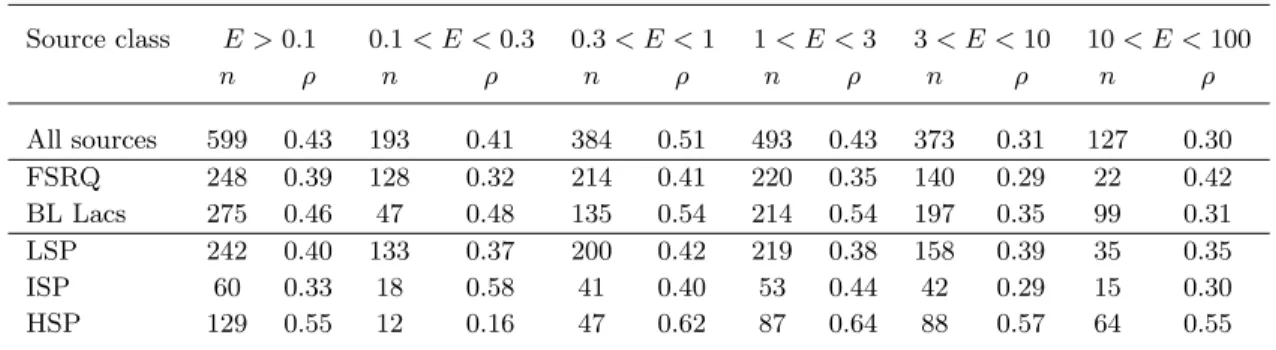
angle with respect to our line of sight.
52
Because most identified gamma-ray AGN are classified as radio-loud objects, a luminosity
53
correlation between those two wavebands appears possible. If proved true, constraints on the
54
physics and location of the jet emission from such AGN may be deduced. Many attempts have
55
been made in the past to investigate correlations between radio (cm)- and gamma-ray luminosities of
56
AGN (e.g., Stecker et al. 1993; Padovani et al. 1993; Salamon & Stecker 1994; Taylor et al. 2007).
57
However, the relation has not been conclusively demonstrated when all relevant biases and selection
58
effects are taken into account (see, e.g. M¨ ucke et al. 1997).
59
For example, while luminosities represent the intrinsic source property, as opposed to fluxes,
60
the use of luminosities always introduces a redshift bias in samples which cover a wide distance
61
range since luminosities are strongly correlated with redshift (Elvis et al. 1978). Such redshift
62
dependence can be removed by means of a partial correlation analysis (see e.g., Dondi & Ghisellini
63
1995). On the other hand, intrinsic correlations between the gamma-ray and radio luminosities
64
may be smeared out, or even lost in the corresponding flux diagrams whereas artificial flux-flux
65
correlations can be induced due to the effect of a common distance modulation of gamma-ray and
66
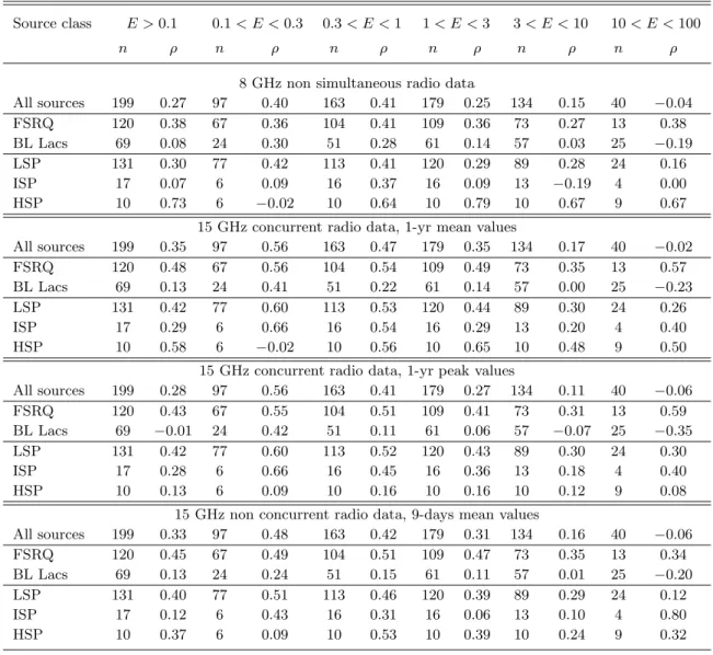
radio luminosities (the “common-distance” bias, see e.g. Pavlidou et al. 2011).
67
Samples that are strongly sensitivity limited restrict the populated region in the luminosity-
68
luminosity diagram to a narrow band, thereby causing serious biases. Therefore, Feigelson & Berg
69
(1983) proposed to include all upper limits to avoid artificial correlations and incorrect conclusions
70
(Schmitt 1985). However, upper limits are usually not distributed randomly in the flux-flux or
71
luminosity-luminosity plane, but are localized in a particular area. In this case, a survival analysis
72
may give misleading results (Isobe 1989). Furthermore, this analysis cannot account for biases
73
caused by misidentification of sources or by truncation effects. Finally, the use of rank correla-
74
tion tests (e.g., Kendall’s
τ, Spearman rank correlation coefficient
ρ) complicates the inclusion of75
observational uncertainties.
76
Another problem is the data and source selection. Blazars are inherently variable sources in the
77
radio as well as the gamma-ray band on a broad range of time scales. Simultaneous observations are
78
therefore the only appropriate data for a correlation analysis. However, due to the lack of such data,
79
the mean (e.g., Padovani et al. 1993) or the brightest flux values (e.g., Dondi & Ghisellini 1995)
80
have often been used instead. As a consequence the dynamical range in the luminosity-luminosity
81
plane is significantly reduced in those cases, and can hence mimic a correlation (M¨ ucke et al. 1997).
82
The question of a correlation between the radio and GeV band on the basis of
Fermidata has re-
83
cently generated a lot of interest and has been the subject of a series of investigations (Kovalev et al.
84
2009; Ghirlanda et al. 2010, 2011; Mahony et al. 2010). However, these studies have been gener-
85
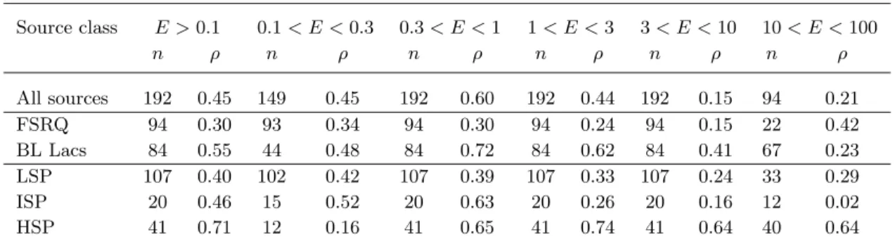
ally limited to a small fraction of the
Fermi-detected AGN and have used non-simultaneous or86
quasi-simultaneous measurements. Moreover, these works have primarily addressed the issue of the
87
apparent strength
of the correlation, rather than that of its
intrinsic significance, which requires a88
dedicated method of statistical analysis. In this paper, we will use the term ”apparent correlation
89
strength” for measures of the tightness of a correlation between radio and gamma-ray
fluxes(such
90
as various correlation coefficients) as seen in the raw data, without applying any correction or sig-
91
nificance assessment to address common-distance bias and the limits on the measured fluxes (the
92
issue of ”censored data”). In contrast, we will use the term ”intrinsic correlation” for the physical
93
correlation between radio and gamma-ray (time-averaged) luminosities, in the limit of an infinite
94
survey, and ”intrinsic correlation significance” for the statistical significance of the claim that a
95
specific dataset exhibits a non-zero intrinsic correlation.
96
In this paper, we revisit this topic exploiting for the first time the
Fermi-LAT data in full, in two97
ways. First, we make use of archival data for about 600 sources, a dataset more than twice as large
98
as that used in Ghirlanda et al. (2010) and Mahony et al. (2010). Second, we take advantage of the
99
large set of concurrent measurements provided by the OVRO monitoring program (Richards et al.
100
2010). The pre-Fermi-launch OVRO sample included
∼200 blazars that are included in the 1FGL
101
catalog, and for which average 15 GHz fluxes measured
concurrentlywith the 1FGL gamma-ray
102
fluxes can be calculated. In addition, we exploit a new statistical method (Pavlidou et al. 2011) to
103
assess the significance of the correlation coefficients.
104
The paper is structured as follows: in Sect. 2, we present the gamma-ray and radio data and
105
the association procedure; the results are presented in Sect. 3 and discussed in Sect. 4 using a
106
dedicated statistical analysis based on the method of surrogate data. A more general discussion is
107
given in Sect. 5 and the main conclusions are summarized in Sect. 6.
108
In the following, we use a ΛCDM cosmology with
h= 0.71, Ω
m= 0.27, and Ω
Λ= 0.73
109
(Komatsu et al. 2009). The radio spectral index is defined such that
S(ν)∝ν−αand the gamma-
110
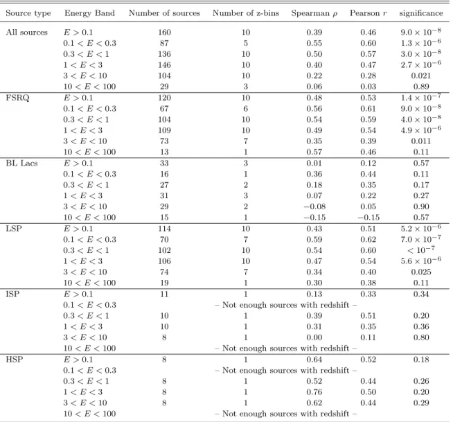
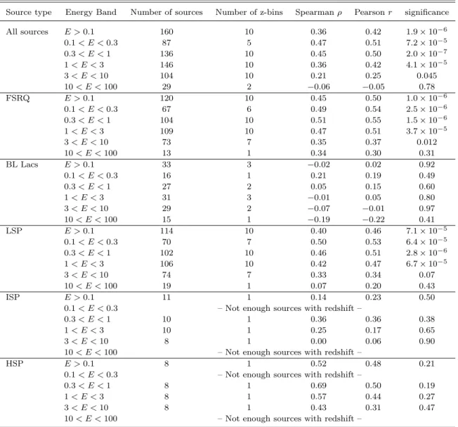
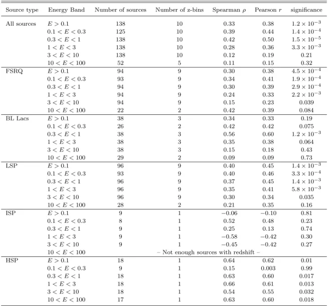
ray photon index Γ such that
dNphoton/dE∝E−Γ.
111
2. Observations and dataset
112
2.1. Gamma-ray data
113
The gamma-ray sources in the present paper are a subset of those in the First
Fermi-LAT cat-114
alog (1FGL, Abdo et al. 2010a). The 1FGL is a catalog of high-energy gamma-ray sources detected
115
by the LAT during the first 11 months of the science phase of
Fermi, i.e. between 2008 August 4116
and 2009 July 4. The procedures used in producing the 1FGL catalog are discussed in detail in
117
Abdo et al. (2010a); in total, the 1FGL contains 1451 sources detected and characterized in the
118
100 MeV to 100 GeV range and belonging to a number of populations of gamma-ray emitters.
119
In general, associations of gamma-ray sources with lower-energy counterparts necessarily rely
120
on a spatial coincidence between the two. A firm counterpart identification requires the search for
121
correlated variability, which is a major effort in the case of AGNs; therefore, only 5 AGNs are listed
122
as firm identifications by Abdo et al. (2010a), although ongoing studies will undoubtedly expand
123
this set. For the rest, associations in 1FGL use a method for finding correspondence between LAT
124
sources and AGNs based on the calculation of association probabilities using a Bayesian approach
125
implemented in the
gtsrcidtool included in the LAT
ScienceToolspackage. A detailed description
126
and a complete list of the source catalogs used by
gtsrcidto draw candidate counterparts can be
127
found in Abdo et al. (2010a).
128
The set of all high-latitude (
|b| >10
◦) 1FGL sources with an AGN association from
gtsrcid129
constitutes the First LAT AGN Catalog (1LAC, Abdo et al. 2010d). Some LAT sources are asso-
130
ciated with multiple AGNs, and consequently, the catalog includes 709 AGN associations for 671
131
distinct 1FGL sources. Each source has an association probability
P, evaluated by examining the
132
local density of counterparts from a number of source catalogs in the vicinity of the LAT source.
133
The main catalogs used are the Combined Radio All-sky Targeted Eight GHz Survey (CRATES;
134
Healey et al. 2007), the Candidate Gamma-Ray Blazar Survey (CGRaBS; Healey et al. 2008), and
135
the Roma-BZCAT (Massaro et al. 2009). Since a few gamma-ray sources have more than one pos-
136
sible association, and not all associations are highly significant, Abdo et al. (2010d) have further
137
defined an AGN “clean” sample consisting of those AGNs that (1) are the sole AGN associated with
138
the corresponding 1FGL gamma-ray source and (2) have an association probability
P ≥80%; a few
139
sources, “flagged” in the 1FGL catalog as exhibiting some problem, have also been discarded and
140
do not belong in the 1LAC clean sample. This clean sample contains 599 AGNs. In the following
141
analysis, whenever we mention the 1LAC sample, we will always be referring to the clean sample
142
even if we do not state so explicitly.
143
For each source in the 1FGL (and hence in the 1LAC), Abdo et al. (2010a) have first obtained
144
good estimates of the significance and the overall spectral slope Γ. Then, in order to obtain good
145
estimates of the energy flux, each of the five energy bands (from 100 to 300 MeV, 300 MeV to 1
146
GeV, 1 to 3 GeV, 3 to 10 GeV, and 10 to 100 GeV) has been fit independently, fixing the spectral
147
index of each source to Γ as derived from the fit over the full interval; finally, the sum of the energy
148
flux in the five bands provided a reliable estimate of the overall flux.
149
In sources with a poorly measured flux (88/599), Abdo et al. (2010a) replaced the value from
150
the likelihood analysis with a 2σ upper limit. However, since these sources are significantly detected
151
when the full band is considered, we estimated their energy fluxes from the flux densities at the
152
pivot energies given by Abdo et al. (2010a), and using the tabulated photon indices and the relative
153
uncertainties on the corresponding quantities. All the obtained data are consistent with the 2σ
154
limits and so have been used for our analysis.
155
We maintain the 1LAC classification of each AGN on the basis of its optical spectrum either
156
as an FSRQ or a BL Lac using the same scheme as in CGRaBS (Healey et al. 2008). In particular,
157
following Stocke et al. (1991), Urry & Padovani (1995), and March˜ a et al. (1996), an object is
158
classified as a BL Lac if the equivalent width (EW) of the strongest optical emission line is
<5 ˚ A,
159
the optical spectrum shows a Ca
IIH/K break ratio
C <0.4, and the wavelength coverage of the
160
spectrum satisfies (λ
max−λmin)/λ
max >1.7 in order to ensure that at least one strong emission
161
line would have been detected if it were present.
162
In addition to the optical spectrum classification, the 1LAC blazars are also classified based
163
on the position of the synchrotron peak, following the scheme proposed by Abdo et al. (2010e); we
164
therefore consider also the three following spectral types: low-synchrotron-peaked blazars (LSP,
165
νpeakS <
10
14Hz); intermediate-synchrotron-peaked (ISP, 10
14Hz
< νpeakS <10
15Hz); or high-
166
synchrotron-peaked (HSP,
νpeakS >10
15Hz). Althought the two classification schemes do have
167
some degeneracy (e.g., HSP sources are largely BL Lacs, while most FSRQs are LSP sources),
168
it is relevant to discuss them both, as the spectral classification is linked to the physical process
169
(synchrotron radiation) responsible for the low frequency emission.
170
In our study we will of course be using only sources that have been associated with a low-
171
energy AGN counterpart. However, we note that 1FGL also contains 374 unassociated sources. If
172
some of these sources are AGN that were not associated with a lower-energy counterpart because
173
they happen to be too faint in radio, then this could potentially introduce a bias in our assessment
174
of the radio/gamma flux correlations. In Fig. 1, we show normalized histograms of the gamma-
175
ray–fluxes of the high-latitude (
|b| >10
◦) AGNs and of the high-latitude unassociated sources.
176
Although in both distributions the sources tend to cluster in the low flux bins, this effect is much
177
more pronounced in the unassociated gamma-ray sources, and there is strong statistical evidence
178
that the two samples are not drawn from the same population (K-S probability of 4.3
×10
−13).
179
This makes it unlikely that we significantly overestimate the strength of the correlation because of
180
the existence of yet-unassociated, radio-faint and gamma-ray-bright blazars.
181
On the other hand, in any given radio flux limited sample there are sources that are radio
182
bright and gamma-ray quiet (see e.g.
§2.2.2 below for the case of the OVRO sample). This fact can
183
be the consequence of long-term variability and/or low duty cycle in gamma-rays (Ghirlanda et al.
184
2011); in any case, in this paper we only deal with the sources detected by LAT.
185
2.2. Radio data
186
In Table 1, we list the radio flux densities used for the present work, along with some basic
187
information on the sources (position, optical and spectral type, redshift). In particular, we give the
188
archival 8 GHz interferometric flux density in Col. 8 (with the corresponding reference in Col. 9)
189
and the 15 GHz single dish flux density, when available, in Cols. 10–12. A summary of the details
190
of the relevant observations are given in the following subsections.
191
2.2.1. CRATES/Other catalogs
192
For all sources in the 1LAC, we were able to collect interferometric measurements of the historic
193
radio flux density. This provides us with the largest database of radio and gamma-ray measurements
194
ever obtained and we use it for a discussion of the correlation between the two bands.
195
Most of these data come from CRATES (478 sources) or CRATES-like (96 sources) observa-
196
tions. The CRATES catalog (Healey et al. 2007) contains precise positions, 8.4 GHz flux densities,
197
and radio spectral indices for over 11,000 flat-spectrum sources over the entire
|b|>10
◦sky. In the
198
region
δ >−40
◦, the 8.4 GHz data were obtained with the VLA in its largest (A) configuration, and
199
the spectral indices were determined by comparing the 8.4 GHz flux density and the 1.4 GHz flux
200
density from the NRAO VLA Sky Survey (NVSS; Condon et al. 1998). In the region
δ <−40
◦, the
201
8.4 GHz data were obtained with ATCA in a variety of large configurations (6A/C/D, 1.5B/C/D),
202
and the spectral indices were determined by comparing the 8.4 GHz flux density and the 843 MHz
203
flux density from the Sydney University Molonglo Sky Survey (SUMSS; Mauch et al. 2003).
1204
The data for sources that are not in CRATES are often of identical or very similar quality
205
to those for CRATES sources. For example, 8.4 GHz data from the Cosmic Lens All-Sky Survey
206
(CLASS; Myers et al. 2003; Browne et al. 2003), from which the CRATES catalog obtained much of
207
its northern hemisphere data in the first place, were all taken with the VLA in the A configuration.
208
Similarly, the PMN-CA catalog
2of over 6600 radio sources was compiled from 8.6 GHz data
209
obtained with ATCA in the 6A, 6C, and 6D configurations. As a result, the radio flux densities
210
and spectral indices of most non-CRATES sources can still be compared directly to those of true
211
CRATES sources without introducing any systematic errors or biases.
212
For 19 sources, for which 8.4 GHz VLA or ATCA measurements are not available, we ex-
213
trapolate from lower frequency interferometric measurements (e.g. those reported from the Roma-
214
BZCAT, Massaro et al. 2009). The spectral indices used for the extrapolation are those available
215
1Strictly speaking, the ATCA observations were performed at 8.6 GHz, and the flux densities were converted to 8.4 GHz by interpolation using the spectral index, but even for a very inverted source (α=−1), this represents an adjustment of<3% to the flux density.
2Survey results can be downloaded from http://www.parkes.atnf.csiro.au/observing/databases/pmn/casouth.pdf
from NED; when none was available, it was conventionally set to
α= 0.0.
216
Finally, there are 6 sources in the 1LAC that possess a significant amount of extended radio
217
emission (such as the misaligned AGNs discussed by Abdo et al. 2010b) and escape the selection
218
criteria of CRATES and similar surveys. However, these are all rather well known radio sources,
219
and it has been straightforward to obtain interferometric measurements of their radio core flux
220
density from the literature, either directly or with trivial calculations (e.g. interpolation).
221
2.2.2. OVRO
222
Since late 2007, the Owens Valley Radio Observatory (OVRO) 40 m Telescope has been en-
223
gaged in a blazar monitoring program to support the
Fermi-LAT (Richards et al. 2010). In this224
program, all 1158 CGRaBS blazars north of declination
−20
◦have been observed approximately
225
twice per week or more frequently since June 2007 (Healey et al. 2008). Gamma-ray blazars and
226
other sources detected by
Fermihave been added to the program which makes the total number of
227
monitored sources close to 1500. Of these sources, 199 appear as “clean” associations in the 1LAC
228
catalog.
229
The OVRO flux densities are measured in a single 3 GHz wide band centered on 15 GHz. Ob-
230
servations were performed using azimuth double switching as described in Readhead et al. (1989),
231
which removes much atmospheric and ground interference. The relative uncertainties in flux density
232
result from a 5 mJy typical thermal uncertainty in quadrature with a 1.6% systematic uncertainty.
233
The absolute flux density scale is calibrated to about 5% via observations of the steady calibrator
234
3C 286, using the Baars et al. model (Baars et al. 1977). A complete description of the OVRO
235
program, population studies of the radio variability, their relation with other physical properties
236
and a study of the time relation between radio and gamma-ray emission are presented in a series
237
of dedicated publications (Richards et al. 2010; Pavlidou et al. 2011; Max-Moerbeck et al. 2011).
238
Because the
Fermi-LAT flux densities used in this study represent time averages over the
239
observation period, we produce estimates of the 15 GHz time average flux density from the OVRO
240
data for each source by linearly interpolating between successive light curve values, integrating
241
between the start and end dates, then dividing by the time interval. For the 11 month data here,
242
the start date was midnight August 4, 2008 (MJD 54682), and the end date was midnight July 4,
243
2009 (MJD 55016). Hereafter, we will be referring to average 15 GHz radio fluxes obtained in this
244
manner as the OVRO
concurrentdata.
245
qThe normalized distribution of average fluxes of the OVRO subset is shown in Fig. 2, over-
246
plotted with the distribution of average fluxes, obtained in the same manner, of gamma-ray quiet
247
CGRaBS sources north of declination
−20
◦. The sources which are also in 1LAC have generally
248
higher 15 GHz average fluxes. However, there is substantial overlap between the two distributions,
249
so the existence of sources with large fluxes at 15 GHz but which are faint in gamma rays is not
250
unexpected. Therefore, our expectation from the distribution of fluxes alone is that if a statistically
251
significant correlation between radio and gamma-ray fluxes indeed exists, it will likely have a
252
substantial scatter.
253
3. Results
254
In this section we present the results of our search for possible correlations between radio flux
255
densities and the gamma-ray photon flux for the sources in the 1LAC sample. In particular, in
256
Sect. 3.1 we consider the full 1LAC sample and search for correlations with archival radio data,
257
while in Sect. 3.2 we focus on the subset of sources observed at OVRO, considering both concurrent
258
and archival radio data; finally, in Sect. 3.3 we present results for a subset of the 1LAC composed
259
of sources detected in at least 4 individual energy bands. There are 599 sources in the 1LAC clean
260
sample and 199 in the 1LAC-OVRO sample. The OVRO 15 GHz concurrent fluxes are averaged
261
(time-integrated, as in the gamma-ray data) over the same interval as the LAT observations, and
262
for all of sources considered here there exists
gamma-rayvariability on timescales shorter than the
263
averaging period.
264
For each sample, we have compared the radio flux density to the 1-yr gamma-ray energy flux
265
at
E >100 MeV. Moreover, since we have unprecedentedly large datasets, we can also explore
266
whether the strengths of any observed correlations are dependent on the gamma-ray energy band
267
in which the flux is calculated, or on the source spectral type. For this reason, we also compare
268
radio flux densities to gamma-ray photon fluxes calculated in the single energy bands 100 MeV
<269
E <
300 MeV, 300 MeV
< E <1 GeV, 1 GeV
< E <3 GeV, 3 GeV
< E <10 GeV, 10 GeV
< E <270
100 GeV. In each energy band, we consider only the sources that are significant in that band. Not
271
every source is detected in all energy bands; actually, only a small minority is, i.e. 51/599 (8.5%).
272
As a consequence of their different spectral properties, FSRQs are generally more abundant in the
273
lowest energy bands, while BL Lacs are more numerous in the most energetic ones. For instance,
274
for the 1LAC sources, we have 128 FSRQs and 47 BL Lacs in the 100–300 MeV band, and 22
275
FSRQs and 99 BL Lacs in the 10-100 GeV band.
276
Since FSRQs and BL Lacs have different spectral properties and showed different behaviors in
277
the preliminary analysis (Abdo et al. 2009; Giroletti et al. 2010), we also tested the two populations
278
separately, in addition to the full set of sources. Moreover, a classification based on the broadband
279
spectral properties is physically more meaningful, so we also consider the populations of low-,
280
intermediate-, and high-synchrotron-peaked blazars (LSP, ISP, and HSP respectively).
281
In total, we have 36 combinations of source type and gamma-ray energy band for the 1LAC.
282
For the OVRO sample, we have also the possibility to consider the radio data obtained at 15
283
GHz during the same interval of the gamma-ray observations, both as mean and peak flux density
284
measurements, and in a different time domain. For each combination, we produced a scatter plot
285
of the radio vs. gamma-ray flux densities and determined the Spearman’s rank correlation
ρ, which286
are presented in the following subsections.
287
The value of
ρis characteristic of the strength of the correlation, and it can be related to
288
the significance of an
apparentcorrelation between radio and gamma-ray fluxes. However, an
289
assessment of the statistical significance of an
intrinsiccorrelation in each case (after the effects
290
of a common distance and a limited dynamical range are accounted for) is nontrivial and cannot
291
be based on a conventional assumption of unbiased samples. Therefore, we use simulations based
292
on the method of surrogated data to evaluate the significance of intrinsic correlations and discuss
293
them in Sect. 4.
294
3.1. Full sample
295
The sources associated to the 1LAC members span over 4 orders of magnitude in radio flux
296
density, ranging between a few mJy for the faintest BL Lacs to several 10’s of Jy for the brightest
297
quasars (e.g. 3C 273 and 3C 279). The flux density distributions for the whole population and
298
divided by source type are shown in Abdo et al. (2010d). The overall distribution shows a broad
299
peak at
S ∼800 mJy, which is the result of the combination of the two peaks of the single
300
population distributions, with BL Lacs peaking around
S ∼400 mJy and FSRQs at
S ∼1300
301
mJy. In gamma-rays, the energy fluxes span over 3 orders of magnitude (between 4.8
×10
−12and
302
6.6
×10
−10erg cm
−2s
−1at
E >100 MeV), with BL Lacs typically fainter than FSRQs; the mean
303
photon fluxes at
E >100 MeV are 8.5
×10
−8ph cm
−2s
−1and 2.9
×10
−8ph cm
−2s
−1for FSRQs
304
and BL Lacs respectively (Abdo et al. 2010d).
305
We show the gamma-ray and radio flux scatter plots for the 1LAC sources in Fig. 3, 4, and 5.
306
Each figure shows a collection of panels showing various combinations of the 1FGL gamma-ray flux
307
and radio historical flux density. In particular, Fig. 3 shows the gamma-ray energy flux vs. radio
308
flux density for all sources (top left panel), sources divided by optical type (FSRQ and BL Lacs in
309
the centre and right top panels, respectively), and sources divided by spectral type (bottom row,
310
with LSP, ISP, and HSP in the left, middle, and right panels, respectively); in Fig. 4 and Fig. 5,
311
we show the gamma-ray photon flux vs. radio flux in the five individual LAT energy bands (left
312
to right), divided by source type: in Fig. 4, the top row shows all sources, the middle one shows
313
FSRQs, and the bottom one BL Lacs; in Fig. 5, top, middle, and bottom rows are for the three
314
different synchrotron peak classes: LSP, ISP, and HSP blazars, respectively. Symbols in magenta
315
show sources for which a redshift is not available.
316
We report the correlation coefficients between radio and gamma-ray flux for the full sample
317
in Table 2, divided by source type and energy band, and we visualize them in Fig. 6. In this
318
figure, the correlation coefficients are shown across the five energy bands and are connected with
319
lines of different color and style for the various sub-populations: solid black line for the full 1LAC
320
sample, dashed lines for optical type sub-groups (red for FSRQ and blue for BL Lacs), dotted lines
321
for sub-groups defined by the spectral properties (magenta for LSP, green for ISP, cyan for HSP).
322
The accuracy to which the correlation coefficients are determined, based on the number of sources
323
and the strength of the correlation, is shown by the error bars, which correspond to the standard
324
deviation for
ρ, defined as σρ= (1
−ρ2)/
√N −
1; although this standard deviation is formally
325
defined only for the Pearson product-moment correlation coefficient
r(Wall & Jenkins 2003), we
326
extend it to our case, since the distribution of the Spearman
ρfor
N >30 approaches that of the
327
Pearson product-moment.
328
The Spearman correlation coefficient for all (599) sources is
ρ= 0.43. FSRQs and BL Lacs
329
reveal different behaviors. In general, BL Lacs exhibit larger values of
ρthan FSRQs, both when
330
the broad band gamma-ray energy flux is considered and in most of the single energy bands;
331
for example, in the most populated energy band (for both populations, the 1–3 GeV band, with
332
220 FSRQ and 214 BL Lacs), we find
ρ= 0.54 for BL Lacs and
ρ= 0.35 for FSRQs, although
333
the difference is less significant in the other energy bands. Moreover, in FSRQs the correlation
334
coefficient is quite stable across the various energy ranges (between
ρ= 0.29 and
ρ= 0.42), while
335
BL Lacs display some evolution, with
ρdecreasing as fluxes at higher energy bands are considered.
336
If one looks at the spectral type populations, HSPs are always the ones showing a tighter apparent
337
correlation (except for the scarcely populated 100–300 MeV band), and as high as
ρ= 0.64 in the
338
1–3 GeV band.
339
3.2. OVRO sample
340
The sources with OVRO data represent a 199 element subset of the 1LAC sample, going down
341
to radio fluxes as low as 172 mJy (archival 8 GHz value for J1330+5202, the source associated
342
to 1FGL J1331.0+5202) and 64.7 mJy (1-yr concurrent 15 GHz value for J1725+1152). FSRQs
343
outnumber BL Lacs by 120/69. This sample provides the largest dataset of concurrent radio
344
measurements to the 1LAC fluxes and is therefore highly valuable in order to understand the
345
implications of variability on the radio/gamma-ray correlation.
346
In particular, we are in the position of comparing the correlation coefficient not only among
347
different source types and energy bands, but also to assess the differences that arise when we use
348
concurrent data or not. In Table 3, we give the correlation coefficients: for the radio/gamma-ray
349
flux densities using historical radio flux densities at 8 GHz; the mean and peak flux density value
350
at 15 GHz calculated over the first 11 months of activity of the LAT; and an average 15 GHz flux
351
calculated over a one-week interval
afterthe first 11 months of activity of the LAT (specifically,
352
the period between January 23 – 31 2010).
353
Figures 7, 8 and 9 show the scatter plots of the concurrent radio and gamma-ray fluxes, using
354
mean values for the radio flux density. As for the 1LAC case, we show 3 collections of scatter plots:
355
radio vs. gamma-ray energy flux for all sources, FSRQ, BL Lacs, LSP, ISP, and HSP sources in
356
Fig. 7, radio vs. gamma-ray photon flux for all sources, FSRQ, and BL Lacs in Fig. 8, and for LSP,
357
ISP, and HSP sources in Fig. 9. Finally, the trend of
ρas a function of energy band for the various
358
sub-classes is shown in Fig. 10, with the same notation as in Fig. 6.
359
Unlike for the larger 1LAC sample, in the sample with concurrently-measured radio fluxes
360
FSRQs generally display larger values of
ρthan BL Lacs; as an example, in the 1–3 GeV energy
361
band,
ρFSRQ= 0.48 and
ρBLL= 0.13. Moreover, the correlation coefficient for BL Lacs for the
362
energy bands above 1 GeV is consistent with no correlation, becoming even marginally negative
363
in the 10–100 GeV band. It has to be remembered that the OVRO sample is somewhat biased
364
in favor of bright radio sources, so it contains relatively few BL Lacs, and in particular just a
365
handful (10/199) of HSPs, as they are generally rather radio weak. Interestingly, the BL Lac curve
366
falls below the three individual spectral type curves (LSP, ISP, HSP). We note that the sample
367
also contains 41 sources (about 20% of the total) whose spectral type is unknown and that have
368
almost uncorrelated radio and gamma-ray flux density. While this explains part of the difference
369
between BL Lacs and LSP+ISP+HSP, it is also important to warn that the 33 LSP BL Lacs do
370
show systematically lower values of
ρthan the whole group of LSP sources (which is dominated by
371
FSRQs).
372
As far as the radio variability is concerned, we find that for the whole sample the correlation
373
coefficient with concurrent 15 GHz data is always larger than that obtained using archival 8 GHz
374
data or non-concurrent 15 GHz OVRO data. This result is mostly driven by the FSRQ population,
375
while the less numerous BL Lac population does not seem to reveal significant differences between
376
the use of concurrent or non-concurrent radio data. Finally, the use of the peak 15 GHz flux
377
density yields generally weaker correlations, in some cases even weaker than those found using
378
non-concurrent data.
379
3.3. Sources significant in at least four energy bands
380
For both the 1LAC and the OVRO samples, we have considered in each energy range all the
381
sources that were significant in that band. As a consequence of the different spectral characteristics
382
of each individual source, the samples used to calculate the various coefficients have often little
383
overlap between each other (even within the same population), particularly in energy bands that
384
are far apart.
385
For this reason, we have also considered a third case, the sample of sources that are significant
386
in at least four of the five individual energy bands. In this way, we build a relatively bright, well
387
defined, and sizable sample. This sample is composed of 192 sources, and both FSRQ (94 sources)
388
and BL Lacs (84) are well represented.
389
As in the full 1LAC sample, BL Lacs have generally higher values of
ρthan FSRQ (e.g.,
390
ρBLL
= 0.54 and
ρFSRQ= 0.29 for the radio vs. energy flux at
E >100 MeV correlation). The
391
individual values are reported in Table 4 and Figs. 11, 12, 13, and 14, using the same notation as
392
in the full 1LAC and OVRO cases.
393
If we look at the three groups defined by the synchrotron spectral properties, we find that the
394
maximum of the correlation coefficient is obtained in the lowest energy band for LSP (ρ = 0.41
395
between 100 and 300 MeV), in the 300 MeV–1 GeV for ISP (ρ = 0.63), and in the 1–3 GeV for HSP
396
(ρ = 0.74). Therefore – albeit with some overlap between the error bars – the higher the spectral
397
frequency of the synchrotron spectral peak, the higher the energy at which the strongest apparent
398
correlation is observed, and the higher the correlation coefficient itself.
399
4. Significance tests with the method of surrogate data
400
In order to quantitatively assess the significance of any apparent correlation between concur-
401
rent radio and gamma-ray flux densities of blazars in the presence of distance effects, we have used a
402
test based on the method of surrogate data. In studying possible intrinsic correlations between flux
403
densities in different bands the null hypothesis is that they are
intrinsicallyuncorrelated (implicitly
404
assuming that any apparent correlation is due to the observational errors and/or biases). In a fre-
405
quentist approach, we investigate how frequently a sample of objects with intrinsically uncorrelated
406
gamma/radio flux densities, similar to the sample at hand, will yield an apparent correlation as
407
strong as the one seen in the data, when subjected to the same distance effects as our actual sample
408
(see Pavlidou et al. 2011, for a more detailed description of the test).
409
In our test the strength of the apparent correlation is quantified by the Pearson product-
410
moment correlation coefficient
r, defined as411
r
=
PN
i=1
(X
i−X)(Y¯
i−Y¯ )
q PN
i=1
(X
i−X)¯
2PNi=1
(Y
i−Y¯ )
2(1)
Since it is not always straightforward to construct simulated samples with the exact same
412
selection criteria as the data sample, we have used
permutationsof measured quantities. To simulate
413
the effect of a common distance on intrinsically uncorrelated luminosities, we permute in luminosity
414
space:
415
•
We split our sample in N redshift bins, with N determined so that each bin has at least
∼10
416
sources. The separation in bins ensures that the luminosity and redshift distributions of the
417
simulated samples approximate those in the real data, thus avoiding the introduction of biases
418
not present in the data. Note however that, as we have shown in detail in Pavlidou et al.
419
(2011), the significance of the correlation we find increases with increasing N (the correlation
420
becomes more significant), until it saturates for large enough N, provided that the number of
421
sources is large enough.
422
•
In each redshift bin: from the measured radio and gamma-ray flux densities, we calculate
423
radio and gamma-ray luminosities at a common rest-frame radio frequency and rest-frame
424
gamma-ray energy.
3425
3In order to implement the K-correction (project our calculated luminosities to a common rest-frame frequency in
•
We permute the evaluated luminosities, to simulate objects with
intrinsically uncorrelated426
radio/gamma luminosities.
427
•
We assign a common redshift (one of the redshifts of the objects in the bin, randomly selected)
428
to each luminosity pair, and return to flux-density space. Returning to flux-density space
429
allows us to avoid Malmquist bias; assigning a common redshift allows us to simulate the
430
common-distance effect on uncorrelated luminosities. In addition, by permuting in luminosity
431
space we are guaranteed that the simulated samples have the same luminosity dynamical range
432
as our actual sample.
433
•
To avoid apparent correlations induced by a single very bright or very faint object
much434
brighter or fainter than the objects in our actual sample, we reject any flux-density pairs
435
where one of the flux densities is outside the flux-density dynamical range in our original
436
sample. The rejection rate is however very low for N
≥3, and it decreases with increasing N.
437
Using a number of flux density pairs equal to the number of objects in our actual sample, we
438
calculate a value for
r. We repeat the process a large number of times, and calculate a distribution of439
r−
values for intrinsically uncorrelated flux densities. The fraction of the area under this distribution
440
for
|r| ≥rdata, where
rdatais the
r−value for the observed flux densities, is the probability to have
441
obtained an apparent correlation at least as strong as a the one seen in the data from a sample with
442
intrinsically uncorrelated gamma-ray/radio emission. This quantifies the statistical significance of
443
the observed correlation.
444
Our results for all the correlations discussed in the present paper are shown in Tables 5 (full
445
1LAC sample), 6 (OVRO sample, using concurrent radio data), 7 (OVRO sample, using non-
446
concurrent radio data), and 8 (sample of sources detected in at least 4 bands); for every case
447
examined, we give the number of sources in the studied subset, the number of redshift bins used in
448
the analysis, the Spearman correlation coefficient
ρ, the value of the Pearson correlation coefficient449
r
of the dataset, and the statistical significance of the apparent correlation, which we define as the
450
fraction of simulated datasets with the same number of points, same common-distance, luminosity-
451
range, and flux-range effects as the actual dataset
but no intrinsic correlationwhich had an absolute
452
value of
rat least as big as the actual dataset. The number of points in each dataset studied
453
generally differs from the number of points in the corresponding dataset of
§3.1, 3.2 and 3.3,
454
because for the surrogate data studies we only use sources for which the redshifts are known. In
455
the scatter plots of Figs. 3–5, 7–9, and 11–13, these sources are plotted with black points (while
456
magenta is used for sources with unknown
z). For the same reason, the Spearman correlation457
each band) we are using the historical radio spectral indexαand the 1FGL photon index; The spectral index has been shown, at least at radio frequencies, to vary with flux (Fuhrmann et al. 2011); however, as shown in Pavlidou et al.
(2011), different choices in radio spectral indices do not have a large effect on the resulting correlation significance, as the sources of interest generally have flat radio spectra and the relevant K-correction is small.