Testing for a constant coefficient of variation in nonparametric regression

Testing for a constant coefficient of variation in nonparametric regression

Holger Dette Ruhr-Universit¨at Bochum

Fakult¨at f¨ur Mathematik 44780 Bochum, Germany e-mail: holger.dette@rub.de

FAX: +49 234 3214 559

Gabriele Wieczorek Ruhr-Universit¨at Bochum

Fakult¨at f¨ur Mathematik 44780 Bochum, Germany e-mail: gabriele.wieczorek@rub.de

November 19, 2007

Abstract

In this paper we propose a new test for the hypothesis of a constant coefficient of variation in the common nonparametric regression model. The test is based on an estimate of theL²- distance between the square of the regression function and variance function. We prove asymptotic normality of a standardized estimate of this distance under the null hypothesis and fixed alternatives and the finite sample properties of a corresponding bootstrap test are investigated by means of a simulation study. The results are applicable to stationary processes with the common mixing conditions and are used to construct tests for ARCH assumptions in financial time series.

Keywords and Phrases: stationary processes, nonparametric regression, constant coefficient of variation, multiplicative error structure, generalized nonparametric regression models.

1 Introduction

We consider the common nonparametric regression model

Y_i =m(X_i) +σ(X_i)ε_i, i= 1,2, . . . , n, (1.1)

wheremdenotes the regression function andσ² the variance function and the random variablesε_i satisfyE[ε_i|X_i =x] = 0 andE[ε²_i|X_i =x] = 1. In many applications the variance can be assumed proportional to the squared mean which corresponds to the assumption of a constant coefficient of variation. Typical examples include models obtained by the logarithmic transformation from regression models with a multiplicative error structure [see Eagleson and M¨uller (1997)] or ARCH- type models [see Engle (1982)]. Several authors have discussed the problem of estimating and testing the regression function under the restriction that m and σ are proportional - see e.g. Mc Cullagh and Nelder (1989), who considered generalized linear models, Carroll and Ruppert (1988), who considered a constant coefficient of variation with a parametric model, and Eagleson and M¨uller (1997), who investigated the common nonparametric regression model under the restriction that m=cσ for some constant c.

In the present paper we will develop a formal test for the hypothesis of a constant coefficient of variation in the nonparametric regression model (1.1), that is

H₀ :m(x) = cσ(x) (1.2)

for some positive (but unknown constant) c. Besides the fact that this test can be used to check the assumptions for a statistical inference in a nonparametric regression model with a constant coefficient of variation, it can also be used as an indicator of a multiplicative error structure (if it is applied to the squares of the data) and an exponentially distributed response Y where E[Y|X = x] = p

Var[Y|X =x] = m(x). In Section 2 we introduce the test statistic and indicate possible applications. Section 3 contains our main results in the case of an i.i.d. sample {X_i, Y_i}ⁿ_i=1. We prove asymptotic normality of a standardized version of the test statistic under the null hypothesis, local and fixed alternatives. In Section 4 we extend these results in the case of stationary time series with the common mixing properties and discuss an application to test for an ARCH(1) model. The finite sample properties of a bootstrap version of the new test are investigated in Section 5 and some of the technical details for the proofs of our main results are presented in the Appendix in Section 6.

2 Testing for a constant coefficient of variation in non- parametric regression

Numerous authors have considered testing various hypotheses regarding the mean and the variance function in the nonparametric regression model (1.1) [see e.g. Dette and Munk (2003) and the

references in this paper]. These hypotheses include parametric and semi parametric assumptions regarding the mean and variance function, but much less effort has been spent in investigating the relation between mean and variance in the nonparametric regression model (1.1). In the present paper we investigate the hypothesis (1.2) of a constant coefficient of variation using an estimate of the L²-distance between the variance and squared regression function. Typical examples include multiplicative models of the form

Y_t =m(X_t)η_t which can be written in the form (1.1) with σ(·) = p

Var (η_t)m(·) and ε_t = (η_t−1)/p

Var(η_t).

Other examples include nonparametric ARCH models X_t =p

m(X_t−1² )η_t, for which the squared process corresponds to a multiplicative times series model.

To be precise let {X_i, Y_i}ⁿ_i=1 denote a bivariate sample of observations from the nonparametric regression model (1.1) with the same distribution and let ˆm and ˆσ² denote two nonparametric estimates of the regression and variance function, respectively, which will be specified in the following section. For any positive c we define the statistic T_n(c) as

Tn(c) = 1 n(n−1)

X

i6=j

Kg(Xi−Xj){c²Y_i²−(c²+ 1) ˆm²(Xi)}w(Xi) (2.1)

× {c²Y_j² −(c²+ 1) ˆm²(X_j)}w(X_j),

where wdenotes a weight function,K_g(·) = _g¹K(·/g),K(·) denotes a kernel andg is a bandwidth converging to 0 with increasing sample size. Note that the statistic of the form (2.1) has been considered before by Zheng (1996) for testing the parametric form of the regression function, by Dette (2002) for testing homoscedasticity, by Dette and von Lieres und Wilkau (2003) and Gozalo and Linton (2000) for testing additivity in a nonparametric regression model (1.1) with a multivariate predictor. If the estimate ˆmis consistent it is intuitively clear that for a large sample size

E[T_n(c)] ≈ E[K_g(X₁ −X₂){c²σ²(X₁)ε²₁−2c²m(X₁)σ(X₁)ε₁−m²(X₁)}

× {c²σ²(X2)ε²₂−2c²m(X2)σ(X2)ε2−m²(X2)}]

≈ E[f(Xi){c²σ²(Xi)−m²(Xi)}²w²(Xi)]

= E[∆²_c(X_i)f(X_i)w²(X_i)], (2.2)

where f denotes the density of X and

∆_c(x) = m²(x)−c²σ²(x).

(2.3)

Note that E[∆²_c(X_i)f(X_i)w²(X_i)] = 0 if and only if the null hypothesis (1.2) is satisfied. There exist a few cases, where the constant c in the statistic T_n(c) is known. For example in ARCH(1) models with standard normal distributed innovations η_t we have X_t² = a₀ + a₁X_t−1² + (a₀ + a₁X_t−1² )(η_t²−1), which givesc= 1/√

2. However, in most cases of practical interest the constant c has to be estimated from the data. For this purpose we consider the least squares problem

ˆ

c² = arg min

c∈IR^>0

Xn

i=1

(m²(X_i)−c²σ²(X_i))²w(X_i) = P_n

i=1m²(X_i)σ²(X_i)w(X_i) P_n

i=1σ⁴(Xi)w(Xi) (2.4)

and estimate the unknown quantities on the right hand side. We define the residuals ˆ

r(X_i) =Y_i−m(Xˆ _i), (i= 1, . . . , n) (2.5)

and the estimate

ˆ

c² = (1/n)P_n

i=1mˆ²(Xi)ˆr²(Xi)w(Xi) (1/n)P_n

i=1(ˆσ²(X_i))²w(X_i) . (2.6)

Note that the squared residuals ˆr²(·) are used for estimating the variance function in the numerator of ˆc² in order to avoid an additional bias caused by the use of the variance estimator ˆσ²(·) [see the proof of Theorem 3.2 in the Appendix].

It is intuitively clear that the expression ˆc² estimates

c²₀ = E[m²(X)σ²(X)w(X)]

E[σ⁴(X)w(X)] , (2.7)

which coincides with the constant c² if the null hypothesis (1.2) is satisfied and corresponds to the best L²-approximation of m² by functions of the form c²σ², otherwise. Consequently the hypothesis of a constant coefficient of variation will be rejected for large values of the statistic T_n(ˆc).

In the following sections we specify the asymptotic properties of the statisticsTn(c), ˆc² andTn(ˆc) if the local linear estimate [see Fan and Gijbels (1996)] is used for estimating the mean and variance function.

3 Main results

In order to state our main results we have to specify nonparametric estimates of the regression and variance function and several assumptions for the model (1.1). We begin with the definition of the estimates. For the regression function we use the local linear estimate [see Fan and Gijbels (1996)]

ˆ m(x) =

P_n

i=1Kh(Xi−x) [sn,2(x)−(x−Xi)sn,1(x)]Yi

P_n

i=1K_h(X_i−x) [s_n,2(x)−(x−X_i)s_n,1(x)]

(3.1)

where K_h(·) = ¹_hK(·/h),K(·) is a kernel,h denotes a further bandwidth and s_n,l(x) =

Xn

i=1

K_h(X_i−x)(x−X_i)^l l = 1,2.

(3.2)

Similarly, the estimate of the variance function is obtained by replacing the observationsY_i by the squared residuals ˆr²(Xi) defined in (2.5) and is given by

ˆ σ²(x) =

P_n

i=1K_h(X_i−x) [s_n,2(x)−(x−X_i)s_n,1(x)] ˆr²(X_i) P_n

i=1K_h(X_i−x) [s_n,2(x)−(x−X_i)s_n,1(x)] . (3.3)

For the sake of transparency we first assume that{X_i, Y_i}ⁿ_i=1 is a sample of independent identically distributed observations. A corresponding result in the time series context is given in the following section. Moreover, the same bandwidths are assumed for the calculation of the estimates of the regression and variance function for the sake of simple notation. The treatment of different bandwidths in these estimates does not cause additional difficulties (and in the simulation study presented in Section 5 we used in fact different bandwidths). Throughout this section we assume that the following assumptions are satisfied

(A1) The density f is twice continuously differentiable on compact sets.

(A2) The regression functionm is four times continuously differentiable on compact sets.

(A3) The variance function σ² is positive and twice continuously differentiable on compact sets.

(A4) The weight function w is twice continuously differentiable and has compact support con- tained in {x|f(x)>0}.

(A5) The kernel K is of order 2, and satisfies a Lipschitz condition.

(A6) If n→ ∞ the bandwidth g and h satisfy

h∼n^−1/5, g=o(h²), ng → ∞.

(3.4)

(A7) The function m_k(x) = E[ε^k|X =x] is continuous for k = 3,4 and for 1≤ k ≤ 8 uniformly bounded, that is

E[ε^k_t|X_t=x]≤C < ∞, k≤8.

(3.5)

(A8) The regression and variance function satisfy

E[m(X)]^k <∞ for k = 2,4, and E[σ²(X)]^k <∞ for k = 1,2.

Our first result specifies the asymptotic distribution of the statistic T_n(c), where the constant c in the hypothesis (1.2) is known. Roughly speaking the statistic T_n(c) is asymptotically normal distributed with different rates of convergence under the null hypothesis and alternative. The proof is complicated and therefore deferred to the Appendix.

Theorem 3.1. Assume that the assumptions (A1) - (A7) are satisfied.

(a) Under the null hypothesis (1.2) we have n√

g Tn(c)−→ N^D (0, µ²₀), (3.6)

where the asymptotic variance is given by

µ²₀ = 2 E[{−1 + 4c²+ 4cm3(X) +m4(X)}²m⁸(X)f(X)w⁴(X)]

Z

K²(u)du.

(3.7)

(b) Under a fixed alternative H₁ :m6=cσ we have

√n(Tn(c)−E[Tn(c)])−→ N^D (0, µ²₁(c)), (3.8)

where

E[Tn(c)] = E[∆²_c(X)f(X)w²(X)] +h²B(c) +o(h²) (3.9)

with ∆_c defined in (2.3), κ₂ =R

u²K(u)du and

B(c) = 2(c²+ 1) κ₂E[∆_c(X)m(X)m⁰⁰(X)f(X)w²(X)].

(3.10)

The asymptotic variance is given by

µ²₁(c) = 4Var(∆²_c(X)f(X)w²(X)) + 16E[∆²_c(X)m²(X)σ²(X)f²(X)w⁴(X)]

+4c⁴E[∆²_c(X)σ⁴(X)f²(X){m₄(X)−1}w⁴(X)]

−16c²E[∆²_c(X)m(X)σ³(X)f²(X)m₃(X)w⁴(X)].

In most applications the value c in the hypothesis (1.2) is not known and has to be estimated from the data. The following results specify the asymptotic properties of the estimate ˆc² defined in (2.6) and the test statistic T_n(ˆc).

Theorem 3.2. If the assumptions (A1) - (A8) are satisfied, then ˆ

c²−E[ˆc²] = 1 n

Xn

i=1

n τ1

³

m²(Xi)σ²(Xi)w(Xi)ε²_i −E[m²(X)σ²(X)w(X)]

´

+ 2τ1m(Xi)σ³(Xi)w(Xi)εi−τ2

³

σ⁴(Xi)w(Xi)−E[σ⁴(X)w(X)]

´ (3.11)

− 2τ₂ σ⁴(X_i)w(X_i){ε²_i −1}

o +o_p

µ 1

√n

¶ .

Moreover,

√n(ˆc²−E[ˆc²])→ N^D (0, ν²), (3.12)

where

E[ˆc²] =c²₀+h²Γ +o(h²) (3.13)

and the constants Γ, τ₁, τ₂ and ν² are given by

Γ = κ₂ E[σ²(X){τ₁m(X)m⁰⁰(X)−τ₂(σ²(X))⁰⁰}w(X)],

τ1 = 1

E[σ⁴(X)w(X)], τ2 = E[m²(X)σ²(X)w(X)]

E²[σ⁴(X)w(X)] ,

ν² = τ₁²Var(m²(X)σ²(X)w(X)) + 4τ₁²E[m²(X)σ⁶(X)w²(X)]

+4τ₁²E[m³(X)σ⁵(X)m₃(X)w²(X)] +τ₂²Var(σ⁴(X)w(X))

+4τ₂²E[σ⁸(X){m₄(X)−1}w²(X)]−2τ₁τ₂Cov(m²(X)σ²(X)w(X), σ⁴(X)w(X))

−4τ₁τ₂E[m²(X)σ⁶(X){m₄(X)−1} w²(X)]−4τ₁τ₂E[m(X)σ⁷(X)m₃(X)w²(X)].

We are now in a position to investigate weak convergence of the statisticT_n(ˆc), where the estimate ˆ

c² is defined in (2.4). We begin with the asymptotic distribution under the null hypothesis (1.2).

Interestingly, in this case the estimation of the scaling factorchas no influence on the asymptotic properties of the test statistic.

Theorem 3.3. Assume that the assumptions (A1) - (A8) are satisfied. Under the null hypothesis (1.2) we have

n√

g T_n(ˆc) =n√

g T_n(c) +o_p(1)−→ N^D (0, µ²₀), where the constant µ²₀ is defined in (3.7).

Our final result in this section refers to the asymptotic properties of the statisticT_n(ˆc) under the alternative. In this case there appears an additional term in the bias and variance of the test statistic, which is caused by the estimation of the scaling factor c. Recall that the constant c²₀ corresponds to the best L²-approximation of m² by functions of the form c²σ².

Theorem 3.4. Assume that the assumptions (A1) - (A8) are satisfied. Under a fixed alternative

%=E[∆_c0(X)σ²(X)f(X)w²(X)]>0

we have

√n(T_n(ˆc)−E[T_n(ˆc)])−→ N^D (0, ω²₁), where

E[T_n(ˆc)] = E[∆²_c0(X)f(X)w²(X)] +h²(B(c₀)−2%Γ) +o(h²),

and B(c₀) is a term in the bias of the statistic T_n(c₀). The asymptotic variance ω₁² is given by ω₁² =µ²₁(c₀) + 4%²ν²−4% υ²(c₀),

where µ²₁(c₀) is defined in Theorem 3.1(b), ν² corresponds to the asymptotic variance of ˆc² in Theorem 3.2 and

υ²(c₀) = 2τ₁E[∆_c0(X)(m²(X)−c²₀σ²(X)m₄(X))m²(X)σ²(X)f(X)w³(X))

−2τ₁E[∆²_c0(X)f(X)w²(X)]E[m²(X)σ²(X)w(X)]

−4c²₀τ₁E[∆_c0(X)m(X)σ⁵(X)f(X)m₃(X)w³(X)]

−2τ2Cov(∆²_c0(X)f(X)w²(X), σ⁴(X)w(X)) +4c²₀τ₂E[∆_c0(X)σ⁶(X)f(X){m₄(X)−1}w³(X)]

+4τ₁E[∆_c0(X)m³(X)σ³(X)f(X)m₃(X)w³(X)]

+8τ₁E[∆_c0(X)m²(X)σ⁴(X)f(X)w³(X)]

−8τ₂E[∆_c0(X)m(X)σ⁵(X)f(X)m₃(X)w³(X)].

Remark 3.5. The term υ²(c₀) corresponds to the asymptotic covariance between the statistic Tn(c0) and the estimate ˆc² of c²₀.

4 Further discussion

4.1 Asymptotic results for absolutely regular processes

The general nonparametric framework includes time series models. Typical examples are multi- plicative models Z_t=σ_tη_t, where σ_t is a positive function of the past {Z_t−i :i≥ 1} and possibly of the past volatility {σ_t−i : i ≥ 1}. For instance, defining σ_t by p

ϑ₀+ϑ₁Z_t−1² for ϑ_i ≥ 0 we achieve the linear ARCH(1) model. Therefore our test can also be used as a preliminary step to identify certain time series. For this purpose it is necessary to extend the asymptotic results under a more general setup which includes both time series data and i.i.d. observations as special cases.

For this purpose we need the following assumptions for some fixed ε∈(0,1/2) and ξ >2.

(M1) The process (X_i, Y_i) is absolutely regular, i.e.

β(k) = sup

s∈Z

E[sup{|P(A|F_−∞^s )−P(A)|A∈ F_s+k^∞ }]→0, as k →0, where F_s^t is theσ-algebra generated by {(X_l, Y_l) :s ≤l ≤t}. Further,

X∞

j=1

j²β^1+εε (j)<∞.

(M2) The innovations ε_t in the model (1.1) satisfy

E[εt|Xt,F_−∞^t−1(X, Y)] = E[εt|Xt] = 0, and

Var(Y_t|X_t,F_−∞^t−1(X, Y)) =σ²(x).

Further, E|ε_t|^k <∞ to the order k≤48ξ(1 +ε).

(M3) The regression function m(·) satisfies

E|m(X)|^k <∞ for k ≤4(1 +ε) and E|m⁰⁰(X)|^k <∞ for k≤20ξ(1 +ε), whereas the variance function σ²(·) fulfills

E|σ²(X)|^k <∞ for k ≤12ξ(1 +ε).

Note that assumption (M3) contains assumption (A8) which is therefore omitted. Under the as- sumptions (A1) - (A7) together with (M1) - (M3) the asymptotic results forT_n(c),ˆc² andT_n(ˆc) can be established for strictly stationary, β-mixing processes {X_i, Y_i}_i∈Z. The proof of the following results is obtained from the proof of the statements presented in Section 3 for the independent case using similar arguments as given by Dette und Spreckelsen (2004), where the authors investigate the asymptotic distribution of goodness-of-fit tests of linearity for absolutely regular processes.

For the sake of brevity the details are omitted and we refer the interested reader to the PhD thesis of Wieczorek (2007). Moreover, we only state the results for the statistic T_n(ˆc). Note that under the null hypothesis the asymptotic distribution of Tn(ˆc) under mixing assumptions coincides with the distribution for the i.i.d. case.

Theorem 4.1 Assume that the assumptions (A1) - (A7) and (M1) - (M3) are satisfied. Under the null hypothesis, we have

n√

g T_n(ˆc)−→ N^D (0, µ²₀), where µ²₀ is the asymptotic variance of T_n(c) defined in (3.7).

Our final theoretical result states the asymptotic properties of the statistic T_n(ˆc) under fixed al- ternatives. Note that in this case the variance of the limit distribution contains the variance of the limit distribution for the i.i.d. case as well as additional covariances. For a precise statement of the result we introduce the notation E^⊗, which denotes the expectation with respect to the product measure.

Theorem 4.2. If the assumptions (A1) - (A7) and (M1) - (M3) are satisfied, then under a fixed alternative % >0 we have

√n¡

Tn(ˆc)−E^⊗[Tn(ˆc)]¢ _D

−→ N(0,ω˜₁²).

In particular,

¯¯E[T_n(ˆc)]−E^⊗[T_n(ˆc)]¯¯=o µ 1

√n

¶ ,

where the mean E^⊗[T_n(ˆc)] and the constant % are given in Theorem 3.4. The asymptotic variance is given by

˜

ω₁² = ˜µ²₁(c0) + 4%²ν˜²−4% υ˜²(c0), (4.1)

where µ˜²₁(c₀) denotes the asymptotic variance of T_n(c₀) defined by

˜

µ²₁(c₀) = µ²₁(c₀) + 8 X∞

t=1

Cov(∆_c0(X₁)[∆_c0(X₁, ε₁) + 2m(X₁)σ(X₁)ε₁]f(X₁)w²(X₁),

∆²_c0(X1+t)f(X1+t)w²(X1+t)),

µ²₁(c₀) is defined in Theorem 3.1(b). The term ν˜² in (4.1) corresponds to the asymptotic variance of the estimate ˆc² given by

˜

ν² = ν²+ 2 X∞

t=1

Cov

³

2τ1m(X1)σ³(X1)w(X1)ε1−τ2σ⁴(X1)w(X1){2ε²₁−1}

+τ1m²(X1)σ²(X1)w(X1)ε²₁, τ1m²(X1+t)σ²(X1+t)w(X1+t)−τ2σ⁴(X1)w(X1)

´ ,

where ν² is given in Theorem 3.2 and υ˜²(c₀) corresponds to the asymptotic covariance between T_n(c₀) and ˆc² defined by

˜

υ²(c0) = υ²(c0) + 2 X∞

t=1

Cov¡

∆c0(X1)f(X1){∆c0(V1) + 2m(X1)σ(X1)ε1}w²(X1),

©τ₁m²(X_1+t)σ²(X_1+t)−τ₂σ⁴(X_1+t)ª

w(X_1+t)¢ + 2

X∞

t=1

Cov¡

∆²_c0(X_1+t)f(X_1+t)w²(X_1+t),

©τ₁m²(X₁)σ²(X₁)ε²₁+ 2τ₁m(X₁)σ³(X₁)ε₁−τ₂σ⁴(X₁)(2ε²₁ −1)ª

w(X₁)¢ , and υ²(c₀) is defined in Theorem 3.4.

Remark 4.3. It is worthwhile to mention that in the case where the stationary process is absolutely regular with a geometric rate, i.e. β(j) = O(ρ^j) for some ρ ∈ (0,1), the asymptotic covariance of the test statistic given in Theorem 4.2 coincides with the asymptotic covariance given in Theorem 3.4 for the independent case, that is:

˜

µ²₁(c₀) =µ²₁(c₀), ν˜² =ν² , ν˜²(c₀) = ν²(c₀) .

Remark 4.4. The moment assumption (M3) is quite restrictive and limits the applicability of the test to many interesting time series models such as ARCH or GARCH models. One possible way to circumvent assumption (M3) is the introduction of an additional weight function in the estimates. As a consequence a slight modification of the estimates can be arranged in our testing procedure eliminating assumption (M3). The details can be found in Wieczorek (2007), and only the modification is mentioned for the sake of brevity. We introduce in a first step an additional weight functionw^∗, satisfying

(A9) w^∗ is twice continuously differentiable and has compact support contained in{x|w(x)>0}.

Next, we propose a modified estimate of the regression function given by ˆm^∗(x) = ˆa, where (ˆa,ˆb) = arg min

a,b

Xn

i=1

{Yi −a−b(Xi −x)}²w(Xi)K

µX_i−x h

¶ (4.2)

is the local linear estimate (additionally weighted by w) of the regression function and its deriva- tive. Note that the modified local linear regression estimator ˆm^∗ differs from the local linear

estimate ˆm in (3.1) by the introduction of the weight function w in (4.2). Similarly, we propose (σ²)^∗(x) = ˆα as the modified estimate of the variance function, where

(ˆα,β) = arg minˆ

α,β

Xn

i=1

©(ˆr^∗)²(Xi)−a−b(Xi−x)ª₂

w^∗(Xi)K

µXi−x h

¶

is the local linear estimate (weighted by the second weight functionw^∗) based on the nonparametric residuals ˆr^∗(X_i) defined by

ˆ

r^∗(X_i) =Y_i−mˆ^∗(X_i).

Based on the modified estimates of the regression function and the variance function the new test statistic is defined by

T_n^∗(c) = 1 n(n−1)

X

i6=j

K_g(X_i−X_j)©

c²Y_i²−(c²+ 1)( ˆm^∗)²(X_i)ª

w^∗(X_i)

ש

c²Y_j²−(c²+ 1)( ˆm^∗)²(Xj)ª

w^∗(Xj).

(4.3)

In addition, we consider the modified least squares problem (ˆc²)^∗ = arg min

c∈IR^>0

Xn

i=1

(m²(X_i)−c²σ²(X_i))²(w^∗)³(X_i).

Therefore, we define the estimate of c² by (ˆc²)^∗ = (1/n)P_n

i=1( ˆm^∗)²(Xi)(ˆr^∗)²(Xi)(w^∗)³(Xi) (1/n)P_n

i=1((ˆσ²)^∗(X_i))²(w^∗)³(X_i) .

As an immediate consequence of the modified definitions the asymptotic results in Theorem 4.1 and 4.2 can also be established for the test statisticT_n^∗(ˆc^∗). No additional assumptions are needed, in particular, the introduction of the weight functions in the estimators avoids the assumption (M3) about the boundedness of the moments of the regression and variance function [see Wiec- zorek (2007) for details]. This modification makes the test applicable to financial time series, as demonstrated in the following section.

4.2 Example: Application to financial time series

The hypothesis of the proportionality of the regression function m and the volatility function σ can also be used to test for a multiplicative model structure. In particular, the proposed test can be viewed as a preliminary step in time series analysis before applying other procedures such as specific testing procedures for ARCH or GARCH models. One important criterion in order

to establish all asymptotic results in such a context is assumption (M3). There the existence of bounds for the absolute moments of the regression function m, its second derivative m⁰⁰ and the variance function σ² is required. But often financial time series do not satisfy this assumption.

For instance, consider the linear ARCH(1) model Z_t=

q

ϑ₀+ϑ₁Z_t−1² η_t

for some constants ϑ₀, ϑ₁ ≥0, ϑ₁ <1, where η_t has mean 0 and variance 1 and is independent of Z_t−1 for all t. The squared ARCH(1) process can be written as

Z_t² = (ϑ₀+ϑ₁Z_t−1² ) + (ϑ₀+ϑ₁Z_t−1² )ε_t, (4.4)

where ε_t = η_t² −1. Clearly, model (4.4) can be identified as a particular case of the general nonparametric regression model (1.1) by taking Y_t = Z_t², X_t = Z_t−1² , m(X_t) = ϑ₀ +ϑ₁X_t and σ(X_t) = c⁻¹(ϑ₀+ϑ₁X_t). The scaling factor cis given by c² = (E[η⁴]−1)⁻¹ and depends only on the error distribution.

For the ARCH(1) process the assumption (M3) can therefore be formulated in terms of the bound- edness of absolute moments of Z_t. So it is important to know whether the stationary solution Z_t has moments of higher orders to apply the test. For stationary ARCH(p) processes with a sym- metric error distribution, a necessary and sufficient condition for the existence of such moments has been given by Milhøj (1985). In particular, let m >0, then the mth moment of an ARCH(1) model exists if and only if E[ϑ1η₀²]^m < 1. As an immediate consequence, one sees that in many cases ARCH processes do not have finite moments of higher orders.

In such cases we refer to Remark 4.4. In order to circumvent the assumption of existing high-order moments ofZ_t we apply the (slightly) modified testing procedure. In particular, the identification of the regression functionmand the variance functionσ² provides the assumptions (A2) and (A3) to be satisfied. Furthermore, from

E[ε^k|X =x] = c^kE[(η²−1)^k|Z_t−1² ] =c^kE[(η² −1)^k]

it follows that (ε_t) fulfills (A7) and (M2) if the innovations η_t satisfy certain moment conditions.

If the assumptions (A1), (A4) - (A7), (A9) are satisfied and the ARCH(1) process (Z_t) fulfills the assumption (M1) the asymptotic normality under the null hypothesis of the corresponding test statistic T_n^∗(ˆc^∗) can be established, that is

n√

g(T_n^∗(ˆc^∗)−E[T_n^∗(ˆc^∗)])→ N^D (0,(µ²₀)^∗), where the asymptotic variance (µ²₀)^∗ is given by

(µ²₀)^∗ = 1152 Z

K²(u)du X8

k=0

µn k

¶

ϑ^n−k₀ ϑ^k₁E[Z^2kf(Z²)(w^∗)⁴(Z²)].

5 Finite sample properties

In order to study the finite sample properties of the new test we have conducted a small simulation study. Because it is well known that the approximation of the nominal level by the normal distribution provided by Theorem 3.3 is not very accurate for moderate sample sizes, we do not recommend to estimate the asymptotic variance and bias and to compare the standardized statistic with the quantiles of a normal distribution. In contrary, we propose to use resampling methods.

As an example we have implemented a smooth bootstrap procedure to obtain the critical values.

For this purpose we estimate the regression and variance function by the local linear estimates defined in (3.1) and (3.3), respectively, and consider the standardized residuals

η_i = Y_i−m(Xˆ _i) ˆ

σ(Xi) i= 1, . . . , n , (5.1)

which are normalized to have mean 0 and variance 1, that is ˆ

ε_i = η_i −η q 1

n−1

P_n

i=1(η_i−η)²

i= 1, . . . , n . (5.2)

The bootstrap errors are then defined as

ε^∗_i = ˜ε^∗_i + vN_i, (5.3)

where ˜ε^∗_i, . . . ,ε˜^∗_n are drawn randomly with replacement from the empirical distribution of the standardized residuals ˆε₁, . . . ,εˆ_n and N₁, . . . , N_n are i.i.d standard normal distributed random variables independent of the sample Y_n = {(X₁, Y₁), . . . , (X_n, Y_n)} and v=v_n is a smoothing parameter converging to 0 with increasing sample size. In the next step bootstrap data is generated according to the model

Y_i^∗ = ˆc ˆσ(Xi) + ˆσ(Xi)ε^∗_i i= 1, . . . , n , (5.4)

where ˆc is the least squares estimate (2.6) obtained from the data corresponding to the range [5%,95%] of the predictors. The test statistic T_n^∗ is calculated from the bootstrap data (X₁, Y₁^∗), . . . ,(X_n, Y_n^∗). If B bootstrap replications have been performed, the null hypothesis (1.2) is rejected if

T_n > T∗(bB(1−α)c)

n ,

(5.5)

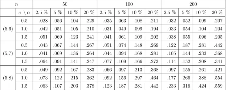
where Tn^∗(1) < < Tn^∗(B) denote the order statistic of the bootstrap sample. For the size of the bootstrap replications we chose B = 100, while 1000 simulation runs are performed for the calculation of the empirical level of this test. The sample sizes are given by n = 50,100,200 and the smoothing parameters in the test statistic and the bootstrap procedure are chosen by

g = n^−1/2 and v = 0.1, respectively. The bandwidths for the estimation of the variance and regression function are chosen separately by least squares cross validation.

Our first example considers the model

m(x) =c(1 + 0.1x) ; σ(x) = (1 + 0.1x), (5.6)

where c = 0.5, 1, 1.5. The predictors X₁, . . . , X_n are independent identically distributed following a uniform distribution on the interval [0,1], while the errors ε₁, . . . , ε_n have a standard normal distribution. The first part of Table 1 shows the approximation of the nominal level, which is rather accurate for sample sizes larger than n= 100. In a second step we study the power of the test and consider the models

m(x) = c(1 + 0.1x) ; σ(x) = (1 + 0.1x+√ x), (5.7)

m(x) =c(1 + 0.1x) ; σ(x) = (1 + 0.1x+ 2√ x). (5.8)

The corresponding results are depicted in the lower part of Table 1. For the model (5.7) we observe a moderate increase in power, which corresponds to intuition. Because the predictor varies in the interval [0,1], the deviation from a multiplicative structure is extremely small for model (5.7). On the other hand, the alternative model (5.8) is detected with larger power, which is also reflected by rather high simulated rejection probabilities.

n 50 100 200

c \α 2.5 % 5 % 10 % 20 % 2.5 % 5 % 10 % 20 % 2.5 % 5 % 10 % 20 % 0.5 .028 .056 .104 .229 .035 .063 .108 .211 .032 .052 .099 .207 (5.6) 1.0 .042 .051 .105 .210 .031 .049 .099 .194 .033 .054 .104 .204 1.5 .051 .069 .123 .241 .041 .061 .109 .202 .038 .055 .096 .205 0.5 .043 .067 .144 .267 .051 .074 .148 .269 .122 .187 .281 .442 (5.7) 1.0 .041 .069 .136 .264 .044 .094 .168 .281 .105 .144 .233 .368 1.5 .064 .091 .141 .247 .077 .109 .166 .273 .114 .152 .208 .341 0.5 .049 .092 .167 .283 .066 .097 .213 .368 .097 .155 .261 .421 (5.8) 1.0 .073 .122 .215 .362 .092 .156 .297 .464 .177 .266 .388 .554 1.5 .063 .107 .203 .378 .123 .187 .281 .442 .233 .316 .424 .559

Table 1: Simulated rejection probabilities of the bootstrap test (5.5), for three nonparametric re- gression models, where the first line corresponds to a multiplicative model.

Our second example investigates the performance of the bootstrap test in the context of stationary time series. To this end we consider two models corresponding to the null hypothesis, that is

Xt= (1 + 0.1Xt−1) + (1 + 0.1Xt−1)εt

(5.9)

X_t = sin(1 + 0.5X_t−1) + sin(1 + 0.5 X_t−1)ε_t (5.10)

and two models corresponding to the alternatives of no multiplicative structure, i.e.

X_t= (1 + 0.1X_t−1) + 0.5p

|X_t−1|ε_t (5.11)

X_t = sin(1 + 0.5X_t−1) + cos(1 + 0.5 X_t1)ε_t (5.12)

where the innovations are again independent standard normal distributed. The corresponding results are displayed in Table 2. We observe a reasonable approximation of the nominal level for the two models corresponding to the null hypothesis. On the other hand, the two alternatives in (5.11) and (5.12) are detected with reasonable power.

n 50 100 200

α 2.5 % 5 % 10 % 20 % 2.5 % 5 % 10 % 20 % 2.5 % 5 % 10 % 20 % (5.9) .029 .047 .097 .217 .023 .048 .089 .187 .024 .048 .097 .189 (5.10) .038 .057 .109 .201 .035 .054 .092 .191 .036 .057 .109 .205 (5.11) .053 .077 .161 .295 .074 .092 .182 .314 .113 .156 .237 .395 (5.12) .084 .117 .189 .299 .097 .133 .212 .321 .129 .176 .289 .417 Table 2: Simulated rejection probabilities of the bootstrap test (5.5) for four nonparametric au- toregressive time series models. The models (5.9) and (5.10) correspond to the null hypothesis of a multiplicative model, while models (5.11) and (5.12) represent the alternative.

6 Appendix: proofs

6.1 Proof of Theorem 3.1.

A straightforward calculation gives the decomposition

T_n(c) = (c²+ 1)²T_1n−2(c²+ 1){2c²T_2n−T_3n(c)}+T_4n(c)−4c²{T_5n(c)−c²T_6n}, (6.1)

with

T_1n = 1 n(n−1)

X

i6=j

K_g(X_i−X_j)δ_n(X_i)w(X_i)δ_n(X_j)w(X_j), T_2n = 1

n(n−1) X

i6=j

K_g(X_i−X_j)δ_n(X_i)w(X_i)m(X_j)σ(X_j)w(X_j)ε_j, T_6n = 1

n(n−1) X

i6=j

K_g(X_i−X_j)m(X_i)σ(X_i)w(X_i)ε_im(X_j)σ(X_j)w(X_j)ε_j, T_3n(c) = 1

n(n−1) X

i6=j

K_g(X_i−X_j)δ_n(X_i)w(X_i)∆_c(X_j, ε_j)w(X_j), T_4n(c) = 1

n(n−1) X

i6=j

K_g(X_i−X_j)∆_c(X_i, ε_i)w(X_i)∆_c(X_j, ε_j)w(X_j), T_5n(c) = 1

n(n−1) X

i6=j

K_g(X_i−X_j)∆_c(X_i, ε_i)w(X_i)m(X_j)σ(X_j)w(X_j)ε_j, where we have used the notation

∆_c(X_i, ε_i) = m²(X_i)−c²σ²(X_i)ε²_i (6.2)

δ_n(X_i) = ˆm²(X_i)−m²(X_i).

(6.3)

At the end of the proof we will show that the terms T1n and T2n are asymptotically negligible under the null hypothesis and under fixed alternatives, that is

n√

g T_jn−→^p 0, j = 1,2.

(6.4)

We now have to distinguish the case of the null hypothesis and alternative.

Proof of Theorem 3.1(a). Note that the statistic T_3n(c) reduces under the null hypothesis to T_3n(c) ^H=⁰ 1

n(n−1) X

i6=j

K_g(X_i−X_j)δ_n(X_i)w(X_i)m²(X_j)w(X_j){1−ε²_j}.

(6.5)

H0

= 2 ˜T_3n⁽¹⁾+ ˜T_3n⁽²⁾ with

T˜_3n⁽¹⁾ = 1 n(n−1)

X

i6=j

K_g(X_i−X_j)m(X_i)˜δ_n(X_i)w(X_i)m²(X_j)w(X_j){1−ε²_j}, T˜_3n⁽²⁾ = 1

n(n−1) X

i6=j

Kg(Xi−Xj)˜δ²_n(Xi)w(Xi)m²(Xj)w(Xj){1−ε²_j},