Testing for symmetric error distribution in nonparametric regression models
Natalie Neumeyer and Holger Dette Ruhr-Universit¨ at Bochum
Fakult¨ at f¨ ur Mathematik 44780 Bochum, Germany
natalie.neumeyer@ruhr-uni-bochum.de holger.dette@ruhr-uni-bochum.de
June 4, 2003
Abstract
For the problem of testing symmetry of the error distribution in a nonparametric re- gression model we propose as a test statistic the difference between the two empirical distribution functions of estimated residuals and their counterparts with opposite signs.
The weak convergence of the difference process to a Gaussian process is shown. The co- variance structure of this process depends heavily on the density of the error distribution, and for this reason the performance of a symmetric wild bootstrap procedure is discussed in asymptotic theory and by means of a simulation study. In contrast to the available procedures the new test is also applicable under heteroscedasticity.
AMS Classification: 62G10, 60F17
Keywords and Phrases: empirical process of residuals, testing for symmetry, nonparametric regression
1 Introduction
Consider the nonparametric heteroscedastic regression model Y
i= m(X
i) + σ(X
i)ε
i(i = 1, . . . , n) (1)
with unknown regression and variance functions m( · ) and σ
2( · ), respectively, where X
1, . . . , X
nare independent identically distributed. The unknown errors ε
1, . . . , ε
nare assumed to be inde- pendent of the design points, centered and independent identically distributed with absolutely continuous distribution function F
εand density f
ε. Hence − ε
ihas density f
−ε(t) = f
ε( − t) and cumulative distribution function F
−ε(t) = 1 − F
ε( − t). In this paper we are interested in testing the symmetry of the error distribution, that is:
H
0: F
ε(t) = 1 − F
ε( − t) for all t ∈ IR versus H
1: F
ε(t) = 1 − F
ε( − t) for some t ∈ IR
1
or equivalently
H
0: f
ε(t) = f
ε( − t) for all t ∈ IR versus H
1: f
ε(t) = f
ε( − t) for some t ∈ IR.
The problem of testing symmetry of the unknown distribution of the residuals in regression models has been considered by numerous authors in the literature for various special cases of the nonparametric regression model (1). Most of the literature concentrates on the problem of testing the symmetry of the distribution of an i.i.d. sample about an unknown mean [see for example Bhattacheraya, Gastwirth and Wright (1982), Aki (1981), Koziol (1985), Schuster and Berker (1987) or Psaradakis (2003) among many others]. Ahmad and Li (1997) transferred an approach of Rosenblatt (1975) for testing independence to the problem of testing symmetry in a linear model with homoscedastic errors. Ahmad and Li’s test was generalized to the nonparametric regression model (1) with homoscedastic errors in the fixed design case by Dette, Kusi–Appiah and Neumeyer (2002). These approaches are based on estimates for the L
2– distance
(f
ε(t) − f
ε( − t))
2dt of the densities f
εand f
−ε. A similar test was proposed recently by Hyndman and Yao (2002) in the context of testing the symmetry of the conditional density of a stationary process.
In this paper we propose an alternative approach for testing symmetry in nonparametric regres- sion models. Our interest in this problem stems from two facts. On the one hand we are looking for a test which is applicable to observations with a heteroscedastic error structure. On the other hand the available procedures for the nonparametric regression model with homoscedastic errors are only consistent against alternatives which converge to the null hypothesis of sym- metry at a rate (n √
h)
−1, where h denotes a smoothing parameter of a kernel estimator. It is the second purpose of this paper to construct a test for the symmetry of the error distribution in model (1), which can detect local alternatives at a rate n
−1/2. To explain the basic idea consider for a moment the regression function m ≡ 0 and variance σ ≡ 1 in model (1) which leads to the well investigated problem of testing the symmetry of the common distribution of an i. i. d. sample ε
1, . . . , ε
n[see e.g. Huˇskova (1984), Hollander (1988) for reviews]. One possible approach is to compare the empirical distribution functions of ε
iand − ε
i[see, for example, Shorack and Wellner (1986, p. 743)] using the empirical process
S
n(t) = 1 n
n i=1I { ε
i≤ t } − I {− ε
i≤ t }
= F
n,ε(t) − F
n,−ε(t), (2)
where I {·} denotes the indicator function, F
n,εis the empirical distribution function of ε
1, . . . , ε
nand F
n,−εis the empirical distribution function of − ε
1, . . . , − ε
n, that is
F
n,−ε(t) = 1 − F
n,ε( − t − ).
Throughout this paper we will call the process S
n(t) (and any process of the same form) empirical symmetry process. Under the hypothesis of symmetry F
ε= F
−εthe process √
nS
nconverges weakly to the process S = B(F
ε) + B (1 − F
ε), where B denotes a Brownian bridge.
The covariance of this limit process is given by
Cov(S(s), S(t)) = F
ε(s ∧ t) − F
ε(s)F
ε(t) + F
ε(( − s) ∧ t) − F
ε( − s)F
ε(t)
+ F
ε(s ∧ ( − t)) − F
ε(s)F
ε( − t) + F
ε(( − s) ∧ ( − t)) − F
ε( − s)F
ε( − t)
= 2F
ε( − ( | s | ∨ | t | )),
(3)
and a suitable asymptotic distribution free test statistic is then obtained by T
n= n
∞0
S
n2(t) dH
n(t),
where H
n= F
n,ε+ F
n,−ε− 1 denotes the empirical distribution function of the absolute values
| ε
1| , . . . , | ε
n| . The test statistic T
nconverges in distribution to the random variable
10
R
2(t) dt, where { R(1 − t) }
t∈[0,1]is a Brownian motion. The null hypothesis of a symmetric error dis- tribution is rejected for large values of this test statistic and the resulting test is consistent with respect to local alternatives converging to the null at a rate n
−1/2. A generalization of the empirical symmetry process (2) for the unknown residuals ε
1, . . . , ε
nin linear models with homoscedastic error structure [that is a regression function m(X
i) = h
T(X
i)β in model (1) with a known function h, finite dimensional parameter β, constant variance function σ(X
i) ≡ σ and a fixed design] can be found in Koul (2002, p. 258).
In the present paper we propose to generalize this approach to the problem of testing the hypoth- esis of a symmetric error distribution in a nonparametric regression model with heteroscedastic error structure. The empirical symmetry process defined in (2) is modified by replacing the unknown errors ε
iby estimated residuals ε
i= (Y
i− m(X
i))/ σ(X
i) (i = 1, . . . , n) where m( · ) and σ( · ) denote kernel based nonparametric estimators for the regression and variance function, respectively. This yields the process
S
n(t) = 1 n
n i=1I { ε
i≤ t } − I {− ε
i≤ t } ,
and allows us also to consider heteroscedastic nonparametric regression models. In Section 3 we prove weak convergence of a centered version of this empirical process to a Gaussian process under the null hypothesis of a symmetric error distribution and any fixed alternative. The covariance structure of the limiting process depends in a complicated way on the unknown distribution of the error and as a consequence an asymptotically distribution free test statistic cannot be found. For this reason we propose a modification of the wild bootstrap approach to compute critical values. The consistency of this bootstrap procedure is discussed in asymptotic theory and by means of a simulation study in Section 4 and Section 5, respectively. The numerical results indicate that the new bootstrap test is applicable for sample sizes larger than 20 and is more powerful than the existing procedures, which were derived under the additional assumption of homoscedasticity.
2 Technical assumptions
In this section we state some basic technical assumptions which are required for the statement of the main results in Section 3 and 4. We assume that the distribution function of the explanatory variables X
i, say F
X, has support [0, 1] and is twice continuously differentiable with density f
Xbounded away from zero. We also assume that the error distribution has a finite fourth moment, that is
E[ε
4] =
t
4f
ε(t) dt < ∞ .
Further suppose that the conditional distribution P
Yi|Xi=xof Y
igiven X
i= x has distribution function
F (y | x) = F
εy − m(x) σ(x)
and density
f (y | x) = 1 σ(x) f
εy − m(x) σ(x)
such that
x∈[0,1]
inf inf
y∈[0,1]
f
F
−1(y | x) | x
> 0 and sup
x,y
| yf (y | x) | < ∞ ,
where F (y | x) and f(y | x) are continuous in (x, y ), the partial derivative
∂y∂f (y | x) exists and is continuous in (x, y) such that
sup
x,yy
2∂f (y | x)
∂y
< ∞ .
In addition, we also require that the derivatives
∂x∂F (y | x) and
∂x∂22F (y | x) exist and are contin- uous in (x, y) such that
sup
x,y
y ∂F (y | x)
∂x
< ∞ , sup
x,y
y
2∂
2F (y | x)
∂x
2< ∞ .
The regression and variance functions m and σ
2are assumed to be twice continuously differen- tiable such that min
x∈[0,1]σ
2(x) ≥ c > 0 for some constant c.
Throughout this paper let K be a symmetric twice continuously differentiable density with compact support and vanishing first moment
uK(u) du = 0 and h = h
ndenote a sequence of bandwidths converging to zero for an increasing sample size n → ∞ such that nh
4= O(1) and nh
3+δ/ log(1/h) → ∞ for some δ > 0.
3 Weak convergence of the empirical symmetry process
We explained in the introduction that the basic idea of the proposed procedure for testing symmetry is to replace the unknown random variables ε
iby estimated residuals ε
i(i = 1, . . . , n) in the definition (2) of the empirical symmetry process. For the estimation of the residuals we define nonparametric kernel estimators for the unknown regression function m( · ) and variance function σ
2( · ) in model (1) by
m(x) =
ni=1
K(
Xih−x)Y
i nj=1
K(
Xjh−x) (4)
σ
2(x) =
ni=1
K(
Xih−x)(Y
i− m(x))
2 nj=1
K(
Xjh−x) . (5)
Note, that m( · ) is the usual Nadaraya–Watson estimator which is considered here for the sake
of simplicity, but the following results are also correct for local polynomial estimators [see Fan
and Gijbels (1996)], where the kernel K has to be replaced by its asymptotically equivalent
kernel [see Wand and Jones (1995)]. Now the standardized residuals from the nonparametric fit are defined by
ε
i= Y
i− m(X
i)
σ(X
i) (i = 1, . . . , n).
(6)
The estimated empirical symmetry process is based on the residuals (6) and given by S
n(t) = F
n,ε(t) − F
n,−ε(t) = 1
n
ni=1
I { ε
i≤ t } − I {− ε
i≤ t } . (7)
Our first result states the asymptotic behaviour of this process.
Theorem 3.1 Under the assumptions stated in Section 2 the process { R
n(t) }
t∈IRdefined by R
n(t) = √
n
S
n(t) − F
ε(t) + (1 − F
ε( − t)) − h
2B (t)
converges weakly to a centered Gaussian process { R(t) }
t∈IRwith covariance structure G(s, t) = Cov(R(s), R(t))
= F
ε(s ∧ t) − F
ε(s)F
ε(t) + F
ε(( − s) ∧ t) − F
ε( − s)F
ε(t)
+ F
ε(s ∧ ( − t)) − F
ε(s)F
ε( − t) + F
ε(( − s) ∧ ( − t)) − F
ε( − s)F
ε( − t) + (f
ε(t) + f
ε( − t))(f
ε(s) + f
ε( − s))
+ (f
ε(s) + f
ε( − s))
t−∞
x(f
ε(x) + f
ε( − x)) dx + (f
ε(t) + f
ε( − t))
s−∞
x(f
ε(x) + f
ε( − x)) dx + s
2 (f
ε(s) − f
ε( − s))
t−∞
(x
2− 1)(f
ε(x) + f
ε( − x)) dx + t
2 (f
ε(t) − f
ε( − t))
s−∞
(x
2− 1)(f
ε(x) + f
ε( − x)) dx + s
2 (f
ε(s) − f
ε( − s))(f
ε(t) + f
ε( − t))E[ε
31] + t
2 (f
ε(t) − f
ε( − t))(f
ε(s) + f
ε( − s))E[ε
31] + st
4 (f
ε(s) − f
ε( − s))(f
ε(t) − f
ε( − t))Var(ε
21), where the bias B(t) is defined by
B(t) = 1 2
K(u)u
2du
(f
ε(t) + f
ε( − t)) 1
σ(x) ((mf
X)
(x) − (mf
X)(x)) dx + t(f
ε(t) − f
ε( − t))
1 2σ
2(x)
(σ
2f
X)
(x) − (σ
2f
X)(x) + 2(m
(x))
2f
X(x) dx
.
Note that the first two lines in the definition of the asymptotic covariance can be rewritten as follows,
F
ε(s ∧ t) − F
ε(s)F
ε(t) + F
ε(( − s) ∧ t) − F
ε( − s)F
ε(t) + F
ε(s ∧ ( − t)) − F
ε(s)F
ε( − t) + F
ε(( − s) ∧ ( − t)) − F
ε( − s)F
ε( − t)
= F
ε(s ∧ t) + 1 − F
ε( − (s ∧ t)) − (F
ε(t) + 1 − F
ε( − t)) + F
ε(( − s) ∧ t) + 1 − F
ε( − ( − s) ∧ t) + (F
ε(t) − 1 + F
ε( − t))(F
ε(s) − 1 + F
ε( − s)),
and under the hypothesis H
0: F
ε(t) = 1 − F
ε( − t) this expression reduces to 2F
ε(s ∧ t) − 2F
ε(t) + 2F
ε(( − s) ∧ t) = 2F
ε( − ( | s | ∨ | t | )),
which coincides with the covariance (3) of the limit of the classical empirical symmetry process (2) based on an i.i.d. sample. Additionally, under H
0we deduce for the bias in Theorem 3.1
B(t) =
K(u)u
2du f
ε(t) 1
σ(x) ((mf
X)
(x) − (mf
X)(x)) dx.
Corollary 3.2 If the assumptions of Theorem 3.1 and the null hypothesis H
0of a symmetric error distribution are satisfied, the process { √
n( S
n(t) − h
2B(t)) }
t∈IRdefined in (7) converges weakly to a centered Gaussian process { S(t) }
t∈IRwith covariance
H(s, t) = Cov(S(s), S(t))
= 2F
ε( − ( | s | ∨ | t | )) + 4f
ε(s)f
ε(t) + 4f
ε(s)
t−∞
xf
ε(x) dx + 4f
ε(t)
s−∞
xf
ε(x) dx.
Comparing the covariance kernel H with the expression (3) we see that there appear three additional terms depending on the density of the error distribution. This complication is caused by the estimation of the variance and regression function in our procedure. We finally note that the bias h
2B(t) in Theorem 3.1 and Corollary 3.2 can be omitted if h
4n = o(1).
Proof of Theorem 3.1:
From Theorem 1 in Akritas and Keilegom (2001) we obtain the following expansion of the estimated empirical distribution function,
F
n,ε(t) = 1 n
n i=1I { ε
i≤ t }
= 1 n
n i=1I { ε
i≤ t } + 1 n
n i=1ϕ(X
i, Y
i, t) + β
n(t) + r
n(t) where, uniformly in t ∈ IR,
r
n(t) = o
p( 1
√ n ) + o
p(h
2) = o
p( 1
√ n )
and
ϕ(x, z, t) = − f
ε(t) σ(x)
(I { z ≤ v } − F (v | x))
1 + t v − m(x) σ(x)
dv
= − f
ε(t) σ(x)
1 − tm(x) σ(x)
∞ z
(1 − F (v | x)) dv −
z−∞
F (v | x) dv
− f
ε(t) σ(x)
t σ(x)
∞ z
v(1 − F (v | x)) dv −
z−∞
vF (v | x) dv
= − f
ε(t) σ(x)
1 − tm(x) σ(x)
(m(x) − z) − f
ε(t)t σ
2(x)
1
2 (σ
2(x) + m
2(x)) − z
22
= − f
ε(t) σ
2(x)
σ(x)(m(x) − z) − tm
2(x) + tm(x)z + 1
2 σ
2(x)t + 1
2 m
2(x)t − 1 2 tz
2. This gives for z = m(x) + σ(x)ε:
ϕ(x, z, t) = ϕ(x, m(x) + σ(x)ε, t) = f
ε(t)
ε + t
2 (ε
2− 1)
.
From the proof of Theorem 1 in Akritas and Keilegom (2001), p. 555, we also have for the bias term
β
n(t) = E
f
ε(t)
m(x) − m(x)
σ(x) dF
X(x) + tf
ε(t)
σ(x) − σ(x)
σ(x) dF
X(x)
= h
22
K(u)u
2du
f
ε(t) 1
σ(x) ((mf
X)
(x) − (mf
X)(x)) dx + tf
ε(t)
1 2σ
2(x)
(σ
2f
X)
(x) − (σ
2f
X)(x) + 2(m
(x))
2f
X(x) dx
+ o(h
2) + o( 1
√ n ).
An analogous expansion for the estimated empirical distribution function F
n,−ε(t) of the signed residuals now yields
S
n(t) = F
n,ε(t) − F
n,−ε(t)
= 1 n
n i=1I { ε
i≤ t } − I {− ε
i≤ t }
= 1 n
n i=1I { ε
i≤ t } − I {− ε
i≤ t } + ε
i(f
ε(t) + f
ε( − t)) + (ε
2i− 1) t
2 (f
ε(t) − f
ε( − t)) (8)
+ h
2B (t) + o
p( 1
√ n )
uniformly with respect to t ∈ IR, where B(t) = (β
n(t) + β
n( − t))/h
2+o(1) is defined in Theorem 3.1. Note, that under the null hypothesis the quadratic term in ε
iin (8), which is due to the estimation of the variance function, vanishes. From the above expansion we obtain
R
n(t) = √ n
S
n(t) − F
ε(t) + (1 − F
ε( − t)) − h
2B(t)
= 1
√ n
ni=1
I { ε
i≤ t } − F
ε(t) − I {− ε
i≤ t } + (1 − F
ε( − t))
+ ε
i(f
ε(t) + f
ε( − t)) + (ε
2i− 1) t
2 (f
ε(t) − f
ε( − t))
+ o
p(1)
= R
n(t) + o
p(1)
uniformly with respect to t ∈ IR, where the last line defines the process R
n. Now a straightfor- ward calculation of the covariances gives:
Cov( R
n(s), R
n(t)) = E
I { ε
1≤ s } − F
ε(s) − I {− ε
1≤ s } + F
−ε(s)) + ε
1(f
ε(s) + f
ε( − s)) + (ε
21− 1) s
2 (f
ε(s) − f
ε( − s))
I { ε
1≤ t } − F
ε(t) − I {− ε
1≤ t } + F
−ε(t)) + ε
1(f
ε(t) + f
ε( − t)) + (ε
21− 1) t
2 (f
ε(t) − f
ε( − t))
+ o(1)
= G(s, t),
where G(s, t) is defined in Theorem 3.1. To prove weak convergence of the process { R
n(t) }
t∈IRwe prove weak convergence of { R
n(t) }
t∈Rand write
R
n(t) = √
n(P
nh
t− P h
t),
where P
ndenotes the empirical measure based on ε
1, . . . , ε
n, that is P
nh
t=
n1 ni=1
h
t(ε
i), P h
tdenotes the expectation E[h
t(ε
i)] and
H = { h
t| t ∈ IR } is the class of functions of the form
h
t(ε) = I { ε ≤ t } − I {− ε ≤ t } + ε(f
ε(t) + f
ε( − t)) + (ε
2− 1) t
2 (f
ε(t) − f
ε( − t)).
To conclude the proof of weak convergence in
∞( H ) we show that the class H is Donsker.
Applying Theorem 2.6.8 (and the remark in the corresponding proof) of van der Vaart and Wellner (1996, p. 142) we have to verify that H is pointwise separable, is a VC–class and has an envelope with finite second moment.
Using the assumptions made in Section 2 we have sup
t∈IR| f
ε(t) | < ∞ , sup
t∈IR| tf
ε(t) | < ∞ and due to this the class H has an envelope of the form
H(ε) = c
1+ εc
2+ (ε
2− 1)c
3,
where c
1, c
2, c
3are constants. This envelope has obviously a finite second moment.
The function class G = { h
t| t ∈ Q I } is a countable subclass of H . For each ε ∈ IR the function t → h
t(ε) is right continuous. Hence for a sequence t
m∈ Q I with t
mt as m → ∞ we have pointwise convergence g
m(ε) = h
tm(ε) → h
t(ε) for m → ∞ . The convergence is also valid in the L
2–sense:
P ((g
m− h
t)
2) ≤ 6
F
ε(t) − F
ε(t
m) + F
−ε(t) − F
−ε(t
m) + E[ε
2](f
ε(t) − f
ε(t
m))
2+ E[ε
2](f
ε( − t) − f
ε( − t
m))
2+ E[(ε
2− 1)
2] 1
4 (tf
ε(t) − t
mf
ε(t
m))
2+ E[(ε
2− 1)
2] 1
4 (tf
ε( − t) − t
mf
ε( − t
m))
2−→ 0 for m → ∞ .
This proves pointwise seperability of H [see van der Vaart and Wellner (1996, p. 116)].
Sums of VC–classes of functions are VC–classes again [see van der Vaart and Wellner (1996, p.
147)]. The classes { ε → I { ε ≤ t } | t ∈ IR } and { ε → I {− ε ≤ t } | t ∈ IR } are obviously VC.
Finally, the function class
{ ε → ε(f
ε(t) + f
ε( − t)) + (ε
2− 1) t
2 (f
ε(t) − f
ε( − t)) | t ∈ IR }
is a subclass of the VC–class { ε → aε + bε
2| a, b ∈ IR } . This yields the VC–property of H and concludes the proof of the weak convergence of the process { R
n(t) }
t∈IR. 2
4 Symmetric wild bootstrap
Suitable test statistics for testing symmetry of the error distribution F
εare, for example, Kolmogorov–Smirnov or Cramer–von–Mises type test statistics,
sup
t∈IR| S
n(t) | and
S
n2(t) d H
n(t), (9)
where H
nis the empirical distribution function of | ε
1| , . . . , | ε
n| and the null hypothesis of symmetry is rejected for large values of these statistics. The asymptotic distribution of the test statistics can be obtained from Theorem 3.1, an application of the Continuous Mapping Theorem and (in the latter case) the uniform convergence of H
n,
sup
t∈IR
| H
n(t) − H(t) | = o
p(1),
where H denotes the distribution function of | ε
1| . A standard argument on contiguity [see e. g. Witting, M¨ uller–Funk (1995), Theorem 6.113, 6.124 and 6.138 or van der Vaart (1998), Section 6] now shows that the resulting tests are consistent with respect to local alternatives converging to the null at a rate n
−1/2. However, because of the complicated dependence of the asymptotic null distribution of the process S
n(t) on the unknown distribution function these test statistics are not asymptotically distribution free. Thus the critical values cannot be computed without estimating the unknown features of the error distribution of the data generating process. To avoid the problem of estimating the distribution and density function F
ε, f
εwe propose a modification of the wild bootstrap approach, which is adapted to the specific problem of testing symmetry.
For this let v
1, . . . , v
nbe Rademacher variables, which are independent identically distributed such that P (v
i= 1) = P (v
i= − 1) = 1/2, independent of the sample (X
j, Y
j), j = 1, . . . , n.
Note that wether the underlying error distribution F
εis symmetric or not the distribution of the random variable v
iε
iis symmetric with density g
εand distribution function G
εdefined by
g
ε(t) = 1
2 (f
ε(t) + f
ε( − t)), G
ε(t) = 1
2 (F
ε(t) + 1 − F
ε( − t)), (10)
respectively. Define bootstrap residuals as follows,
ε
∗i= v
i(Y
i− m(X
i)) = v
iσ(X
i) ε
i(i = 1, . . . , n)
where ε
iis given in (6). Now we build new bootstrap observations (i = 1, . . . , n) Y
i∗= m(X
i) + ε
∗i= v
iσ(X
i)ε
i+ m(X
i) + v
i(m(X
i) − m(X
i)) and estimated residuals from the bootstrap sample,
ε
i∗= Y
i∗− m
∗(X
i)
σ
∗(X
i) , (11)
where the regression and variance estimates m
∗and σ
∗2are defined analogous to m and σ
2in (4) and (5) but are based on the bootstrap sample (X
i, Y
i∗), i = 1, . . . , n. In generalization of definition (7) the bootstrap version of the empirical symmetry process is now defined as
S
n∗(t) = F
n,ε∗(t) − F
n,−ε∗(t) = 1 n
n i=1I { ε
i∗≤ t } − I {− ε
i∗≤ t } .
The asymptotic behaviour of the bootstrap process conditioned on the initial sample is stated in the following theorem. Note that the result is valid under the hypothesis of symmetry f
ε= f
−εand under the alternative of a non-symmetric error distribution.
Theorem 4.1 Under the assumptions of Theorem 3.1 the bootstrap process { √
n( S
n∗(t) − h
2B(t)) }
t∈IR,
conditioned on the sample Y
n= { (X
i, Y
i) | i = 1, . . . , n } , converges weakly to a centered Gaussian process { S(t) }
t∈IRwith covariance
Cov(S(s), S(t)) = 2G
ε( − ( | s | ∨ | t | )) + 4g
ε(s)g
ε(t) + 4g
ε(s)
t−∞
xg
ε(x) dx + 4g
ε(t)
s−∞
xg
ε(x) dx in probability, where the bias term is defined by
B(t) =
K(u)u
2du g
ε(t) 1
σ(x) ((mf
X)
(x) − (mf
X)(x)) dx.
Here g
εand G
εare given by (10) and under the null hypothesis of symmetry we have g
ε= f
ε, G
ε= F
εand Cov(S(s), S(t)) = H(s, t), where the kernel H(s, t) is defined in Corollary 3.2.
The proof of Theorem 4.1 is deferred to the Appendix.
From the theorem the consistency of a test for symmetry based on the wild bootstrap procedure can be deduced as follows. Let T
ndenote the test statistic based on a continuous functional of the process S
nand let T
n∗denote the corresponding bootstrap statistic based on S
n∗. If t
nis the realization of the test statistic T
nbased on the sample Y
nthen a level α–test is obtained by rejecting symmetry whenever t
n> c
1−α, where P
H0(T
n> c
1−α) = α. The quantile c
1−αcan now be approximated by the bootstrap quantile c
∗1−αdefined by
P (T
n∗> c
∗1−α| Y
n) = α.
(12)
From Theorem 4.1 and the Continuous Mapping Theorem we obtain a consistent asymptotic
level α–test by rejecting the null hypothesis if t
n> c
∗1−α. We will illustrate this approach in a
finite sample study in Section 5.
5 Finite sample properties
In this section we investigate the finite sample properties of the bootstrap procedure proposed in Section 4 by means of a simulation study. Exemplarily we consider the statistic
T
n=
S
n2(t)d H
n(t), (13)
where
H
n(t) = 1 n
n i=1I {| ε
i| ≤ t }
denotes the empirical distribution function of the absolute residuals | ε
1| , . . . , | ε
n| . If T
n∗=
( S
n∗)
2(t) d H
n∗(t)
is the bootstrap version of T
n, where H
n∗= F
n,ε∗+ F
n,−ε∗− 1 denotes the empirical distribution function of | ε
1∗| , . . . , | ε
n∗| , the consistency of the bootstrap procedure follows from Theorem 4.1, the Continuous Mapping Theorem and the fact that for all δ > 0 we have
P
sup
t∈IR
| H
n∗(t) − H(t) | > δ Y
n= o
p(1).
For the bandwidth in the regression and variance estimator defined by (4) and (5), respectively, we used
h = σ
2n
3/10, (14)
where
σ
2= 1 2(n − 1)
n−1 i=1(Y
[i+1]− Y
[i])
2(15)
is an estimator of the integrated variance function
10
σ
2(t)f
X(t)dt and Y
[1], . . . , Y
[n]denotes the ordered sample of Y
1, . . . , Y
naccording to the X values [see Rice (1984)]. The same bandwidth was used in the bootstrap step for the calculation of ε
∗1, . . . , ε
∗nand the corresponding estimators
m
∗, σ
∗.
B = 200 bootstrap replications based on one sample Y
n= { (X
i, Y
i) | i = 1, . . . , n } were per- formed for each simulation, where 1000 runs were used to calculate the rejection probabilities.
The quantile estimate c
∗1−αdefined in (12) from the bootstrap sample T
n∗,1, . . . , T
n∗,Bwas defined by
c
1−α∗= T
n∗,(B(1−α)),
where T
n∗,(i)denotes the ith order statistic of T
n∗,1, . . . , T
n∗,B. The null hypothesis H
0of a symmetric error distribution was rejected if the original test statistic T
nbased on the sample Y
nexceeded c
1−α∗.
The model under consideration was
Y
i= sin(2πX
i) + σ(X
i)ε
i, i = 1, . . . , n,
(16)
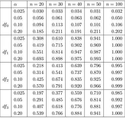
for the sake of comparison with the results of Dette, Kusi-Appiah and Neumeyer (2002), who proposed a test for symmetry in a nonparametric homoscedastic regression model with a fixed design. Table 5.1 shows the approximation of the nominal level for the uniform design on the interval [0, 1]. The error distribution is a normal distribution, a convolution of two uniform distributions and a logistic distribution standardized such that E[ε] = 0, E[ε
2] = 1, while the variance function is constant i.e. σ(x) ≡ 1. We observe an accurate approximation of the nominal level for sample sizes n ≥ 20.
The performance of the new test under alternatives is illustrated in Table 5.2, where a standard- ized chi-square distribution with k = 1, 2, 3 degrees of freedom is considered. The non-symmetry is detected in all cases with high probability, where the power increases with the sample size and decreases with increasing degrees of freedom. The cases k = 1, 2 should be compared with the simulation results in Dette, Kusi-Appiah and Neumeyer (2002), where the same situation for a fixed design has been considered. We observe notable improvements with respect to the probabilities of rejection in all considered cases. We note again that the procedure of these authors requires a homoscedastic error, while the bootstrap test proposed in Section 4 is also applicable under heteroscedasticity.
In order to investigate the impact of heteroscedasticity on the approximation of the level and the probability of rejection under the alternative we conducted a small simulation study for the case m(x) = sin(2πx), σ(x) = e
−x√
2(1 − e
−2)
−1/2, a normal distribution and chi-squared distribution with k = 1, 2, 3 degrees of freedom standardized such that E[ε] = 0, E[ε
2] = 1. The explanatory variable is again uniformly distributed on the interval [0, 1]. Note that the variance function was normalized such that
10
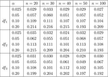
σ
2(x)dx = 1 in order to make the results comparable with the scenario displayed in Table 5.1 and 5.2. The results are presented in Table 5.3. We observe no substantial differences with respect to the approximation of the nominal level (compare the first case in Table 5.1 and 5.3) and a slight loss with respect to power, which is caused by the heteroscedasticity (compare the cases df
1, df
2and df
3in Table 5.3 with Table 5.2). The results indicate that our procedure has a good performance under heteroscedasticity.
α n = 20 n = 30 n = 40 n = 50 n = 100 0.025 0.029 0.033 0.029 0.029 0.027 0.05 0.057 0.060 0.051 0.057 0.052 df
10.10 0.109 0.111 0.107 0.107 0.104 0.20 0.214 0.216 0.215 0.193 0.209 0.025 0.035 0.032 0.024 0.032 0.029 0.05 0.062 0.055 0.051 0.068 0.057 df
20.10 0.113 0.111 0.101 0.113 0.108 0.20 0.215 0.209 0.204 0.210 0.193 0.025 0.031 0.030 0.028 0.028 0.030 0.05 0.055 0.051 0.061 0.049 0.067 df
30.10 0.108 0.101 0.112 0.102 0.105 0.20 0.199 0.204 0.202 0.197 0.192
Table 5.1: Simulated level of the wild bootstrap test of symmetry in the nonparametric re-
gression model (16) with σ(x) ≡ 1. The error distribution is a normal distribution (df
1), a
logistic distribution (df
2) and a sum of two uniforms (df
3) standardized such that E[ε] = 0 and E[ε
2] = 1.
k α n = 20 n = 30 n = 40 n = 50 n = 100 0.025 0.358 0.654 0.849 0.957 1.000 0.05 0.484 0.764 0.912 0.981 1.000 1 0.10 0.584 0.847 0.959 0.991 1.000 0.20 0.716 0.914 0.983 0.998 1.000 0.025 0.239 0.458 0.698 0.817 0.998 0.05 0.342 0.570 0.805 0.896 1.000 2 0.10 0.442 0.681 0.865 0.936 1.000 0.20 0.594 0.794 0.934 0.976 1.000 0.025 0.208 0.436 0.604 0.750 0.982 0.05 0.303 0.565 0.710 0.833 0.995 3 0.10 0.414 0.667 0.812 0.895 0.998 0.20 0.551 0.790 0.886 0.939 0.999
Table 5.2: Simulated power of the wild bootstrap test of symmetry in the nonparametric re- gression model (16) with σ(x) ≡ 1. The error distribution is a chi-square distribution with k degrees of freedom standardized such that E[ε] = 0 and E[ε
2] = 1.
α n = 20 n = 30 n = 40 n = 50 n = 100 0.025 0.030 0.033 0.034 0.031 0.032 0.05 0.056 0.061 0.063 0.062 0.050 df
00.10 0.094 0.113 0.107 0.101 0.106 0.20 0.185 0.211 0.191 0.211 0.202 0.025 0.308 0.610 0.838 0.941 1.000 0.05 0.419 0.715 0.902 0.969 1.000 df
10.10 0.551 0.814 0.947 0.987 1.000 0.20 0.693 0.898 0.975 0.993 1.000 0.025 0.218 0.413 0.639 0.796 0.995 0.05 0.314 0.541 0.737 0.870 0.997 df
20.10 0.425 0.674 0.835 0.925 0.999 0.20 0.570 0.791 0.920 0.966 0.999 0.025 0.197 0.377 0.559 0.710 0.985 0.05 0.291 0.485 0.676 0.814 0.992 df
30.10 0.407 0.618 0.776 0.881 0.997 0.20 0.539 0.766 0.884 0.941 1.000
Table 5.3: Simulated level and power of the wild bootstrap test of symmetry in the nonparamet- ric regression model (16) with σ(x) = √
2e
−x(1 − e
−2)
−1/2. The error distribution is a standard
normal distribution (df
0) and chi-square distribution with k degrees of freedom (df
k, k = 1, 2, 3)
standardized such that E [ε] = 0, E[ε
2] = 1.
A Appendix: Proof of Theorem 4.1
We decompose the residuals ε
∗idefined in (11) in the following way,
ε
i∗= v
iσ(X
i)
σ
∗(X
i) ε
i+ v
im(X
i) − m(X
i)
σ
∗(X
i) + m(X
i) − m
∗(X
i)
σ
∗(X
i) . Hence for t ∈ IR the inequality ε
i∗≤ t is equivalent to
v
iε
i≤ td
∗n2(X
i) + v
id
n1(X
i) + d
∗n1(X
i) and v
iε
i≤ t is equivalent to
v
iε
i≤ td
n2(X
i) + v
id
n1(X
i), where we introduced the definitions
d
n1(x) = m(x) − m(x)
σ(x) , d
n2(x) = σ(x) σ(x) , d
∗n1(x) = m
∗(x) − m(x)
σ(x) , d
∗n2(x) = σ
∗(x) σ(x) .
In the following we need four auxiliary results which are listed in Proposition 4.2–4.5 and can be proved by similar arguments as given in Abritas and Keilegom (2001). For the sake of brevity we will only sketch a proof of Proposition A.1 at the end of the general proof. The verification of Proposition A.2 follows from a Taylor expansion as in the proof of Theorem 1 of Akritas and Keilegom (2001) while the proof of Proposition A.3 follows exactly the lines of the proof of Lemma 1, Appendix B, in this reference. The proof of Proposition A.4 is done by some straightforward calculations of expectations and variances and is therefore omitted.
Proposition A.1 Under the assumptions of Theorem 3.1 we have 1
n
ni=1
I { ε
i∗≤ t } − P (vε ≤ td
∗n2(X) + vd
n1(X) + d
∗n1(X) | Y
n)
− I { v
iε
i≤ t } + P (vε ≤ td
n2(X) + vd
n1(X) | Y
n)
= o
p( 1
√ n ) uniformly in t ∈ IR.
Proposition A.2 Under the assumptions of Theorem 3.1 we have
P (vε ≤ td
∗n2(X) + vd
n1(X) + d
∗n1(X) | Y
n) − P (vε ≤ td
n2(X) + vd
n1(X) | Y
n)
− P ( − vε ≤ td
∗n2(X) − vd
n1(X) − d
∗n1(X) | Y
n) + P ( − vε ≤ td
n2(X) − vd
n1(X) | Y
n)
= 2g
ε(t)
m
∗(x) − m(x)
σ(x) dF
X(x) + o
p( 1
√ n )
uniformly in t ∈ IR, where g
εis defined in (10).
Proposition A.3 Under the assumptions of Theorem 3.1 we have 1
n
ni=1
I { v
iε
i≤ t } − I { v
iε
i≤ t } − P (vε ≤ td
n2(X) + vd
n1(X) | Y
n) + P (vε ≤ t)
= o
p( 1
√ n ) uniformly in t ∈ IR.
Proposition A.4 Under the assumptions of Theorem 3.1 we have m
∗(x) − m(x)
σ(x) dF
X(x) = h
2B (t)/(2g
ε(t)) + 1 n
n j=1ε
jv
j+ o
p( 1
√ n )
where B(t) is defined in Theorem 4.1.
From Proposition A.1, an analogous result for the empirical distribution function F
n,−ε∗(t) =
n1
ni=1
I {− ε
i∗≤ t } , and Proposition A.2 we have uniformly with respect to t ∈ IR [see also the identity (8) in the proof of Theorem 3.1 and note that g
εis symmetric]
S
n∗(t) − h
2B(t) = 1 n
n i=1I { ε
i∗≤ t } − I {− ε
i∗≤ t }
− h
2B(t)
= 1 n
n i=1I { v
iε
i≤ t } − I {− v
iε
i≤ t }
+ 2g
ε(t)
m
∗(x) − m(x)
σ(x) dF
X(x)
− h
2B (t) + o
p( 1
√ n ).
Now an application of Proposition A.3, an analogous result for F
n,−ε∗(t), and Proposition A.4 yields
S
n∗(t) − h
2B(t) = 1 n
n i=1I { v
iε
i≤ t } − I {− v
iε
i≤ t }
+ P (vε ≤ td
n2(X) + vd
n1(X) | Y
n)
− P (vε ≤ t) − P ( − vε ≤ td
n2(X) − vd
n1(X) | Y
n) + P ( − vε ≤ t) + 2g
ε(t) 1
n
nj=1
ε
jv
j+ o
p( 1
√ n )
= 1 n
n i=1I { v
iε
i≤ t } − I {− v
iε
i≤ t } + 2g
ε(t)ε
iv
i+ o
p( 1
√ n )
= 1 n
n i=1v
iI { ε
i≤ t } − I {− ε
i≤ t } + 2g
ε(t)ε
i+ o
p( 1
√ n ),
where in the last two equalities we have used P (v
i= 1) = P (v
i= − 1) = 1/2. By an application of Markov’s inequality we obtain, conditional on Y
n, that the processes √
n( S
n∗(t) − h
2B(t)) and
R
∗n(t) = 1
√ n
ni=1