Testing symmetry of a nonparametric bivariate regression function

SFB 823

Testing symmetry of a Testing symmetry of a Testing symmetry of a Testing symmetry of a nonparametric bivariate nonparametric bivariate nonparametric bivariate nonparametric bivariate regression function

regression function regression function regression function

D is c u s s io n P a p e r

Melanie Birke, Holger Dette, Kristin Stahljans

Nr. 5/2009

Testing symmetry of a nonparametric bivariate regression function

Melanie Birke

, Holger Dette and Kristin Stahljans

Fakult¨at f¨ ur Mathematik

Ruhr-Universit¨at Bochum, Germany July 10, 2009

Abstract

We propose a test for symmetry of a regression function with a bivariate predictor based on theL₂ distance between the original function and its reflection. This distance is estimated by kernel methods and it is shown that under the null hypothesis as well as under the alternative the test statistic is asymptotically normally distributed. The finite sample properties of a bootstrap version of this test are investigated by means of a simulation study and a possible application in detecting asymmetries in gray-scale images is discussed.

1 Introduction

Symmetric structures play an important role in many contexts in science, art and the real world (see e.g. Weil, 1952, Rosen, 1995 or Conway et al., 2008). Most parts of the human body are nearly symmetric, for example, the right hand is more or less symmetric to the left hand. By modeling this mathematically the problems reduce to symmetry of functions. For example, a symmetric grey-scale image is a symmetric function of the pixel location taking values between 0 and 1 or a distribution of some characteristics in a population modeled as random variables is symmetric if the underlying density is symmetric. So, most models of this kind can be reduced to symmetry of regression functions or densities and the problem of testing for symmetry is of particular interest for these functions. There exists already some work on tests for symmetry of densities. Huˇskov´a (1984) proposes a test for symmetry of the common distribution of two p-dimensional random vectors. Hollander (1988) gives an overview of several tests for symmetry of distribution or density functions. In Ahmad and Li (1997) a test for symmetry of a density function based on kernel methods is proposed. A test based on transformed empirical processes is given in Caba˜na and

1Adress for correspondance: Melanie Birke, Ruhr-Universit¨at Bochum, Fakult¨at f¨ur Mathematik, Univer- sit¨atsstraße 150, 44780 Bochum, Germany, e-mail: melanie.birke@rub.de,Fon: +49/234/32–23286, Fax:

+49/551/32–14559

Caba˜na (2000), while Dette, Kusi-Appiah and Neumeyer (2002) develop a test for symmetry of the error distribution in regression models.

In the present paper we discuss the problem of testing for symmetry of a regression function, which is of similar importance as the problem of testing for symmetry of density functions. Our work is motivated by some applications in thermographic image analysis, where abnormalities such as malignancies, inflammation and infection cause localized increases in temperature which show as asymmetrical patterns in an infrared thermogram [see for example Gratt et. al (1995), Jones (1998), Kruganti and Qi (2002) among many others]. In such cases – besides the visual inspec- tion of the images – statistical tests for the symmetry of the regression function are of interest to detect asymmetries at a controlled significance level. A typical application will be given in Sec- tion 4.2. Moreover, such tests can also be used generally in image analysis to test, whether an underlying object is symmetric with respect to some (known) axis or has some symmetric compo- nents. Additionally, the knowledge of symmetry is for example of advantage in image compression or reconstruction.

There already exist various methods in the literature addressing the issue of symmetry of objects or functions. They can generally be classified in two groups. One group consists of methods for determining a symmetry axis in images or functions or, more general, for fixing regions of (local) symmetries in two-dimensional objects. We mention here the work of Atallah (1985), Friedberg (1986), Marola (1989), Kiryathi and Gofman (1998), Loy and Zelinsky (2003) or Xiao et al. (2005) among others. In most of these articles it is assumed, that the regression function or image is observed without any stochastic errors. The second group is concerned with the question if, given an image or data, an object or regression function is symmetric with respect to some known or unknown axis. Recently, Bissantz, Holzmann and Pawlak (2009) propose tests for reflection sym- metry and rotational invariance of two-dimensional regression functions or images based on Zernike polynomials. On the other hand statistical tests based on kernel regression estimates do not exist so far, especially in multivariate settings. On the one hand such methods are attractive because of their simplicity - they are usually based on a direct comparison of the functions estimating the images. On the other hand statistical tests based on kernel regression estimates also provide, beside the result of a statistical test, an estimate of a simply interpretable measure for the deviation from the null hypothesis. For example, if symmetry with respect to the y-axis has to be tested, the test proposed in this paper will be based on a kernel estimate of the quantity

I = Z

A

(m(x, y)−m(−x, y))²d(x, y), (1.1) and the null hypothesis of symmetry is rejected for large values of the corresponding estimate. The L²-distance I can be considered as a measure for asymmetry and further statistical inference could be performed using estimates of this quantity. Moreover, as pointed out by Rosenblatt (1975) or

Ghosh and Huang (1991) kernel based tests are usually powerful with respect to local alternatives of the form

m(x, y) = m(−x, y) +βnω

x−c1

ηn

,y−c2

ηn

(1.2) where βn, ηn→0, c1, c2 ∈R(see Remark 1 in Section 3).

In the present paper we propose a test for symmetry of a regression function with a two dimensional predictor based on kernel regression estimates. Although there are various characterizations of sym- metry of a function, we investigate the fundamental one, which is motivated by several applications in thermographic image analysis, i.e.

H0 : m(−x, y) = m(x, y) for allx, y . (1.3) Note that we assume that the axis of symmetry is known. If this is not the case, it has to be estimated first. Then, the general case can be easily traced back to the case investigated below.

The remaining part of this paper is organized as follows. In Section 2 we define the test statistic and give a heuristic motivation. In Section 3 the asymptotic properties of the test statistic are investigated under the nullhypothesis and the alternative, and we also show the consistency of the test which rejects the null hypothesis (1.3) for large values of the estimate for the L²-distance defined in (1.1). The applicability of the test is demonstrated in Section 4 where we show some simulation results and apply the procedure to an example from image analysis. The proofs are all deferred to the Appendix.

2 The test statistic and basic assumptions

We consider the nonparametric regression model with a bivariate predictor

Zi = m(Xi, Yi) +σ(Xi, Yi)εi i= 1, . . . , n . (2.1) Throughout this paper we restrict ourselves to the situation of symmetry with respect to they-axis and assume that observations are available on the set A= [−1,1]². The hypotheses are

H0 : m(x, y) =m(−x, y) for almost all (x, y)^T ∈[−1,1]²,

H1 : there exists a set B ⊂[−1,1]² with positive Lebesgue measure such that m(x, y)6=m(−x, y) for all (x, y)^T ∈B.

All methods can be easily modified for testing symmetry with respect to the x axis or even with respect to any other axis. If the true regression function m is symmetric in the first component,

then this should also hold approximately for any consistent estimator ˆmofm. Therefore we propose to estimate the distance I in (1.1) by

Iˆn = Z

A

[ ˆm(x, y)−m(ˆ −x, y)]²d(x, y) (2.2) and to reject the null hypothesis for large values of this test statistic, where ˆm is an estimator of the regression function. If the null hypothesis of symmetry is true, the statistic ˆIn converges in probability to 0 as long as ˆm is uniformly consistent, which intuitively explains why this procedure should yield a consistent test. In principle any consistent estimate could be used in this procedure but for the sake of brevity, we restrict ourselves to the Nadaraya-Watson and the local linear estimate in the following discussion. The Nadaraya-Watson estimate is defined by

ˆ

m^{N W}(x, y) = 1

na₁a₂fˆ_n(x, y)kXi−x a1

,Yi−y a2

Zi

with

fˆn(x, y) = 1 na1a2

n

X

i=1

kXi−x a1

,Yi−y a2

,

and if this estimate is used in (2.2), the resulting statistic will be denoted by ˆI_n^{N W} in the following discussion. Similarly the two-dimensional local linear estimator for a kernel k and a bandwidth (a₁, a₂)^T is defined by

ˆ

m0,1(x, y) = h

(S2,0(x, y)S0,2(x, y)−S_0,2² (x, y))T0,0(x, y)

+(S1,0(x, y)S1,1(x, y)−S0,1(x, y)S2,0(x, y))T0,1(x, y)(S0,1(x, y)S1,1(x, y)−S0,2(x, y)S1,0(x, y))T1,0(x, y)i

×h

2S0,1(x, y)S1,0(x, y)S1,1(x, y)−S0,2(x, y)S_1,0² (x, y)−S0,0(x, y)S_1,1² (x, y)−S_1,0² (x, y)S2,0(x, y) +S0,0(x, y)S0,2(x, y)S2,0(x, y)i−1

, where

Sj,k(x, y) =

n

X

i=1

kXi−x a1

,Yi−y a2

(Xi−x)^j(Yi−y)^k

Tj,k(x, y) =

n

X

i=1

kXi−x a1

,Yi−y a2

(Xi−x)^j(Yi−y)^kZi. and the resulting statistic in (2.2) is denoted by

Iˆ_n,0,1 = Z

A

( ˆm_0,1(x, y)−mˆ_0,1(−x, y))d(x, y)

throughout this paper. For the sake of transparency, we assume for the asymptotic considerations in the following that a1 =a2 =h and k(u, v) =k1(u)k2(v) where k1 and k2 are univariate kernels.

However, all results presented here remain valid in the general case with an additional amount of notation. Obviously critical values can only be obtained by asymptotic considerations, which require knowledge of the asymptotic distribution of the statistic In under the null hypothesis and under the alternative. Roughly speaking, it will be shown in the next section that an appropriately scaled version of the statistic In is asymptotically normally distributed under the null hypothesis and the alternative, where different rates appear in both cases. We conclude this section with a statement of the necessary assumptions for these asymptotic results.

Assumption 1

1. The random variables (Xi, Yi), i = 1, . . . , n are independent and identically distributed with density f whose support contains the set

A^δ ={z ∈R²|inf

a∈A||z−a|| ≤δ}.

2. The error variablesεi,i= 1, . . . , nare independent and identically distributed with E[εi] = 0, E[ε²_i] = 1 and existing finite fourth moment µ4 = E[εi] and independent of the sequence {(Xi, Yi)}ⁿi=1.

Assumption 2

1. The regression function m and the density f are two times continuously differentiable with uniformly continuous second derivative.

2. The function σ:A^δ→R⁺ of the standard deviation of Zi is continuous.

Assumption 3

1. The symmetric kernelsk₁ and k₂ are of order 2 and have compact support, say [−1,1].

2. The bandwidth h is proportional to the optimal bandwidth for two-dimensional regression estimation, that is h=Cn^−1/6.

3 Weak convergence under the null hypothesis and alter- native

For the construction of an asymptotic level α test based on the statistic ˆIn in (2.2) we need the (1−α)-quantile of the asymptotic distribution of the test statistic ˆIn under the null hypothesis.

Our first theorem states that in this case the test statistic converges weakly with rate nh to a normal distribution. Throughout this paper g1∗g2 denotes the convolution of the functionsg1 and g2, and for a function g the symbol∂jg denotes the partial derivative of g with respect to the j-th component.

Theorem 1 Let the assumptions 1 - 3 stated in Section 2 be fulfilled. Then τ_n⁻¹

Iˆ_n^{N W} −µn

_D

→ N(0,1), (3.1)

where µn = E[Sn], τn =

4

n²h²α1+16h⁴ n α2

1/2

Sn = Z

A

[ ˆm^{N W}(x, y)−mˆ^{N W}(−x, y)]²fˆ_n²(x, y) ˆf_n²(−x, y)

E[ ˆf_n(x, y)]²E[ ˆf_n(−x, y)]² d(x, y) α1 = 2

Z

[(k∗k)(u, v)]²d(u, v) Z

A

σ²(x, y)hσ²(x, y)

f²(x, y) + σ²(−x, y) f(x, y)f(−x, y)

id(x, y), α₂ =

Z

A

σ²(x, y)γ²(x, y)

f³(x, y)f²(−x, y)d(x, y) and

γ(x, y) = Z 1

−1

k₁(u)u²du[f(−x, y)∂₁f(x, y)−f(x, y)∂₁f(−x, y)]∂₁m(x, y) +

Z 1

−1

k2(v)v²dv[f(−x, y)∂2f(x, y)−f(x, y)∂2f(−x, y)]∂2m(x, y),

The proof of this result is complicated and therefore deferred to the Appendix. If m and f are at least three times continuously differentiable, the bias term simplifies substantially, that is µn in (3.1) can be replaced by

˜

µn = 1 nh²

Z

A

σ²(x, y)

f(x, y) + σ²(−x, y) f(−x, y)

d(x, y)

Z

k²(u, v)d(u, v) +h⁴ Z

A

γ(x, y) f(x, y)f(−x, y)

2

d(x, y).

If the alternative H₁ : I 6= 0 holds, then we observe a different asymptotic behavior of the test statistic T_n. For a statement of the precise result we introduce the following notation

Tn = 1 h²

Z

A

[Zi−m(x, y)]k1

Xi−x h

k2

Yi−y h

[m(x, y)−m(−x, y)]

E[ ˆfn(x, y)] d(x, y)

τ² = Z

A

σ²(u, v)(m(u, v)−m(−u, v))²

f(u, v) d(u, v)

(3.2)

Theorem 2 Let the assumptions of Theorem 1 be fulfilled. If the regression function m is not symmetric then

√n( ˆI_n^{N W} −I−4bn)→ N^D (0, τ²), (3.3) where bn = E[Tn].

If the regression and density function are at least three times continuously differentiable, the bias term bn in (3.3) can be replaced by

˜b_n = h²

κ₂(k₁)(∂₁²m(x, y)f(x, y)−∂₁m(x, y)∂₁f(x, y)) +κ₂(k₂)(∂₂²m(x, y)f(x, y)−∂₂m(x, y)∂₂f(x, y))

×m(x, y)−m(−x, y) f(x, y) .

From Theorem 1 and 2 the asymptotic distribution of the test statistic under the null hypothesis and the alternative the following result can easily be obtained.

Corollary 1 Under the assumptions of Theorem 2 the test which rejects the null hypothesis of symmetry for large values of the statistic Iˆ_n^{N W} is consistent.

Remark 1 It can be shown by similar arguments as given in the Appendix, that for alternatives of the form (1.2) with a square integrable twice continuously differentiable function ω and

β_n = 1

√nh^1+2δ η_n =h^δ

(δ >1/2) the statistic on the left hand side of (3.1) is also asymptotically normally distributed with variance 1 and mean proportional to R

w²(x)dx. Because the size of the integral Z c₁

−∞

Z c₂

−∞

βnw((x−c1)η_n⁻¹,(y−c2)η⁻¹_n )dydx is of order

βnη_n² =n^−1/2h^(1+2δ)/2h^2δ =n^−1/2h^δ−1/2 =n^−1/2n^{−(δ−1/2)/6},

the test proposed in this paper has greater power against such local alternatives than tests based on empirical processes [see Rosenblatt (1975) or Ghosh and Huang (1991) for more details].

Remark 2

(A) By Theorem 1 an asymptotic and consistent level α test for the hypothesis of symmetry is obtained by rejecting the null hypothesis if ˆI_n^{N W} − µˆn > τˆnz1−α, where ˆµn,τˆn are appropriate

(consistent) estimates of µn and τn, respectively, and z1−α denotes the (1− α) quantile of the standard normal distribution. It now follows from Theorem 2 that the power of this test can be approximated by

P(H0 rejected | H1 is true) ≈ 1−Φ −√

n(I+ 4bn)/τ +√

n(µn+τnz1−α)/τ

. (3.4) where µn, τn and bn are defined in Theorem 1 and 2, respectively. This formula provides also information about the behavior of the power function, which depends (asymptotically) on the particular alternative only through the three quantities bn, I and τ².

(B) Note that the quantity I defined in (1.1) can be interpreted as a measure of symmetry of the regression function. From Theorem 2 we obtain under the alternative

Iˆ_n^{N W} −4bn+ τ˜_nz_1−α

√n

as an upper (asymptotic) (1−α) confidence bound for the parameterI, where ˜τ_n² is an appropriate (consistent) estimator of the asymptotic variance given in Theorem 2.

(C) A further important application of Theorem 2 arises from the fact that in practice - in particular when analyzing thermal images - perfect symmetry will usually never be observed. The more realistic question in this context is, if there exists approximately symmetry. Therefore we propose to investigate the so called precise hypotheses [see Berger and Delampady (1987)]

H0 :I > ε versus H1 :I ≤ε , (3.5)

where I is the measure defined by (1.1) and ε > 0 is a prespecified constant for which the exper- imenter agrees to accept the image as symmetric. An asymptotic α-level test for the hypothesis (3.5) is obtained by rejecting the null hypothesis, whenever

√n( ˆI_n^{N W} −ε−4b_n)<τˆ_nz_1−α.

We conclude this section with the corresponding statements for the local linear case. Note that the discussion presented in Remark 1 and 2 is also valid for this type of estimate.

Theorem 3 If the assumptions of Theorem 1 are satisfied, we have under the null hypothesis

nhα^−1/2_0,1 ( ˆIn,0,1−EX[ ˆIn,0,1])→ N^D (0,1), (3.6) where EX denotes the conditional expectation with respect to X ={(X1, Y1), . . . ,(Xn, Yn)} and

α0,1 = 2 Z

(k∗k)²(u, v)d(u, v) Z

A

σ²(x, y)hσ²(x, y)

f²(x, y) + σ²(−x, y) f(x, y)f(−x, y)

id(x, y).

Under the alternative I >0 it follows that

√nτ^−1/2( ˆI_n,0,1−EX[ ˆI_n,0,1])→ N^D (0,1), (3.7) whereτ is defined in Theorem 2. Ifmis at least three times continuously differentiable, the centering term EX[ ˆI_n,0,1] in (3.6) and (3.7) can be replaced by

1 nh²

Z

A

σ²(x, y)

f(x, y) + σ²(−x, y) f(−x, y)

d(x, y) Z

k²(u, v)d(u, v) and

I+h² Z

A

(κ2(k1)∂₁²m(x, y) +κ2(k2)∂²₂m(x, y))(m(x, y)−m(−x, y))d(x, y), respectively.

4 Finite sample properties and a data example

In this section we study the finite sample behavior of the test based on the L²-distance by means of a simulation study and an application.

4.1 Simulated examples

Although Theorem 1 and 3 specify the asymptotic behavior of the statistics ˆI_n^{N W} and ˆIn,0,1, we have so far no information about the size and power of the test in finite samples. One typical problem in the application of tests based on an L²-distance between nonparametric regression estimates is, that the asymptotic distribution still depends on certain parameters of the data generating process, which are often difficult to estimate. Moreover, even if the asymptotic variance and bias in Theorem 1 can be estimated the approximation of the nominal level is usually rather poor [see e.g. Fan and Linton (2003)]. Hence, we propose to use a wild bootstrap version of the test which is often used in heteroscedastic regression models [see e.g. Wu (1986) or H¨ardle and Mammen (1993)]. For this purpose we form a bootstrap sample (X1, Y1, Z₁^∗), . . . ,(Xn, Yn, Z_n^∗) from (X1, Y1, Z1). . . ,(Xn, Yn, Zn) with

Z_i^∗ = ˆmS(Xi, Yi) +Ciεˆi, i= 1, . . . , n.

In this definition we use the symmetrized regression estimator ˆ

mS(x, y) = m(x, y) + ˆˆ m(−x, y)

2 ,

the estimated residuals

ˆ

εi =Zi−m(Xˆ i, Yi), i= 1, . . . , n

-1 -0.5 0 0.5 1 -1

-0.5 0 0.5 1

-1 -0.5 0 0.5 1

-1 -0.5 0 0.5 1

-1 -0.5 0 0.5 1

-1 -0.5 0 0.5 1

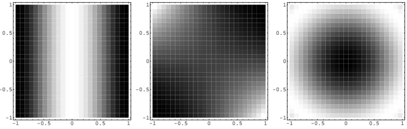
Figure 1: Contour plots of the regression functions m1, m2 and m3 with a = 0 (from left to right).

and independent identically distributed random variables Ci which are independent of the sample (X1, Y1, Z1), . . . ,(Xn, Yn, Zn) and are drawn from the distribution which puts mass (√

5 + 1)/2√ 5 at the point (1−√

5)/2 and mass (√

5−1)/2√

5 at the point (1 +√

5)/2. From this bootstrap sample we calculate the bootstrap version ˆI_n^∗ of the test statistic. After B repetitions of the bootstrap procedure we obtain a sample

Iˆ_n,1^∗ , . . . ,Iˆ_n,B^∗

of the test statistics, which can be used to estimate the (1−α)-quantile of the distribution under the null hypothesis by the ⌊(1−α)B⌋-th order statistic, say ˆIn,(⌊(1−α)B⌋)^∗ . Therefore the null hypothesis of symmetry is rejected if

Iˆn>Iˆn,(⌊(1−α)B⌋)^∗ . (4.1)

The consistency of this bootstrap procedure follows by similar arguments as presented in the proof of Theorem 1 (see the Appendix) along the lines given in H¨ardle and Mammen (1993) or Dette and Neumeyer (2001), who prove consistency of the wild bootstrap in the context of testing parametric assumptions and comparing regression curves.

We restrict the investigations of the finite sample properties to the local linear estimator because of its advantages with respect to boundary effects. We use least squares cross validation to determine the bandwidth for the estimation of the regression function in the test statistic ˆIn,0,1 and the errors ˆ

εi. For the symmetric estimate ˆms required in the construction of the bootstrap sample we use a slightly larger bandwidth to ensure a correct estimation of the bias.

For our simulation study we consider the following regression functions m1(x, y) = (1−x²)²

m2(x, y) = (1−xy)²

m3,a(x, y) = sin((x−a)²+y²), a= 0,0.005,0.0075,0.01.

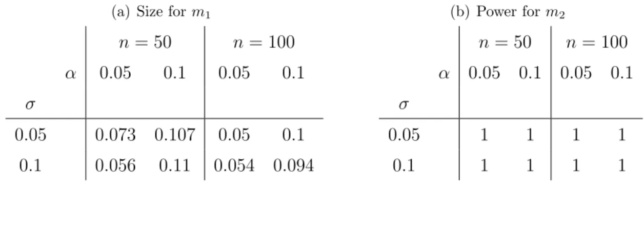
Table 1: Size and power of the test (4.1) for the symmetry of the regression functions m1 and m2

estimated from 500 simulation runs for α = 0.05 and α= 0.1.

(a) Size form

1

n = 50 n= 100

α 0.05 0.1 0.05 0.1

σ

0.05 0.073 0.107 0.05 0.1 0.1 0.056 0.11 0.054 0.094

(b) Power form

2

n= 50 n= 100 α 0.05 0.1 0.05 0.1 σ

0.05 1 1 1 1

0.1 1 1 1 1

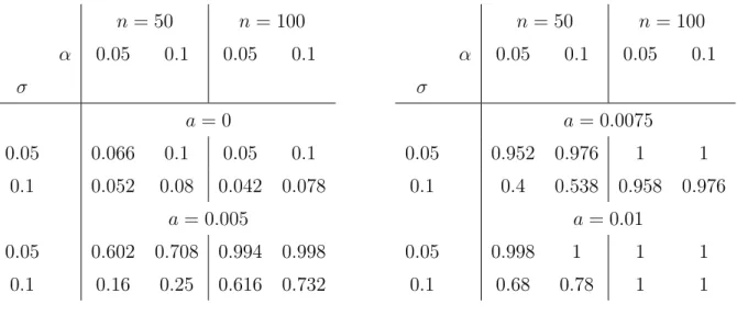
The first regression function is symmetric and the second one is not symmetric. The third one is symmetric with respect to the y axis for a = 0. For a = 0.005, 0.0075 and 0.01, it is shifted to the right and therefore not symmetric with respect to the y axis. Contour plots of these functions are presented in Figure 1. We consider a uniform design on [−1,1]², normally distributed errors with different standard deviations σ and different α. The sample sizes are n = 50 and 100 while the number of bootstrap replications in each simulation run is B=200. The size and power of the test is estimated from 500 simulation runs. The results for the three different regression functions are presented in Tables 1 and 2 for the regression functions m1 and m2, respectively. We observe that for the regression function m1 the nominal level is approximated very well in both cases σ = 0.05 and σ = 0.1. For the function m2, which is not symmetric with respect to the y-axis, the simulated power is 100% in all cases. For a more detailed investigation of the behaviour of the test under alternatives we consider the function m3 for different values ofa. The simulation results are presented in Table 2. We see that a small shift (a = 0.005) is harder to detect than a larger shift (a= 0.0075 or a= 0.01), especially for larger standard deviations. But in all cases where the regression function m3 is not symmetric to the y-axis, the simulated power is considerably higher than the size of the test. The simulations also show (as expected), that the power is smaller for a higher standard deviation of the errors.

4.2 Testing gray-scale images for symmetry

Gray-scale images can be understood as a two dimensional regression problem. Every pixel is defined by its horizontal position xi and its vertical position yi in the picture and has a value Zi ∈ [0,1]

defining its scale of gray. Without loss of generality we may assume, that the coordinates (xi, yi), i= 1, . . . , n of every pixel are located in the set [−1,1]² so that the origin of the coordinate system

Table 2: Size and power of the test (4.1) for the symmetry of the regression function m3,a estimated from 500 simulation runs for α = 0.05 and α= 0.1.

n = 50 n= 100

α 0.05 0.1 0.05 0.1

σ

a= 0

0.05 0.066 0.1 0.05 0.1

0.1 0.052 0.08 0.042 0.078 a = 0.005

0.05 0.602 0.708 0.994 0.998 0.1 0.16 0.25 0.616 0.732

n = 50 n= 100

α 0.05 0.1 0.05 0.1

σ

a = 0.0075

0.05 0.952 0.976 1 1

0.1 0.4 0.538 0.958 0.976 a= 0.01

0.05 0.998 1 1 1

0.1 0.68 0.78 1 1

is located in the center of the image. In many cases the images are disturbed by error terms ε_i. Therefore the image of a symmetric object usually does not show perfect symmetry. Only knowing the image of an object, this evokes the question if the real object can be symmetric with respect to the vertical or horizontal axis.

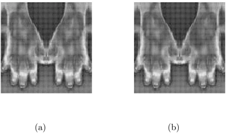
We now illustrate the application of the new test in the context of analyzing thermographic images, which are used in medicine to detect diseases, especially inflammations in parts of the human body [see for example Gratt et. al. (1995), Jones (1998) or Kuruganti and Qi (2002)]. While most parts of the human body are nearly symmetric concerning the thermographical characteristics (e.g. left and right hand/arm/leg etc.) an inflammation e.g. of a finger violates this symmetry between the left and right hand. In Figure 2 we show two thermographic images of a right hand and its reflection.

The image in Figure 2(a) exhibits symmetry. The image in 2(b) has a small modification which violates the symmetry. We now use the new bootstrap test to check the symmetry with respect to the centered vertical axis in both cases. For the image in Figure 2(a), the p-value of the test is 0.232 and therefore the null hypothesis is not rejected at significance level α = 0.05. On the other hand for the image in Figure 2(b) thep-value is 0 and therefore the test rejects the null hypothesis.

Thus the asymmetry is clearly detected.

(a) (b)

Figure 2: Thermographic image of a hand: (a) duplicated and mirrowed image of a right hand (perfect symmetry) disturbed with errors. (b) duplicated and mirrowed image of a right hand with modification in the right part of the image (small deviation from symmetry) disturbed with errors.

5 Concluding Remarks

In this paper we have developed a consistent test for symmetry of a bivariate regression function with respect to a known axis using kernel methods. As natural application we showed an example from image analysis with a more or less continuous change of grey scales. This assumption is not always plausible for all images because there are often edges where colours change abruptly. Then the standard kernel estimates do not provide useful estimates and modifications like e.g. in Gijbels, Lambert and Qiu (2007), Hall, Qiu and Rau (2008) or wavelet estimators might provide better results.

Image analysis can always be seen as inverse problem and testing for symmetry of the true regression function is then of special interest if the point spread function is not symmetric. Topics of current research are therefore testing for symmetry with respect to an unknown axis and in inverse problems.

Acknowledgements The authors would like to thank Stephanie S¨ohnel for her assistance with the simulations and Martina Stein, who typed parts of this manuscript with considerable technical expertise. This work has been supported in part by the Collaborative Research Center ”Statistical modeling of nonlinear dynamic processes” (SFB 823) of the German Research Foundation (DFG).

References

I.A. Ahmad (1982). Nonparametric estimation of the location and scale parameters based on density estimation. Annals Inst. Statist. Math. 34, 39-53.

I.A. Ahmad and Q. Li (1997). Testing symmetry of an unknown density function by kernel method.

Nonparam. Statist. 7, 279-293.

M.J. Atallah (1985). On symmetry detection. IEEE Trans. Comput. C-34, 663-666.

L. Baringhaus and N. Henze (1992). A characterization of and new consistent tests of symmetry.

Commun. Statist. 21, 1111-1125.

J.O. Berger and M. Delampady (1987). Testing precise hypotheses. Statist. Sci., 2, 317-352.

M. Birke (2008). Central limit theorems for the integrated squared error of derivative estimators.

Statist. Probab. Lett. 78, 1903–1913.

Bissantz, Holzmann and Pawlak (2009). Testing for Image Symmetries – with Application to Confocal Microscopy. IEEE Trans. Information Theory, to appear.

A. Caba˜na and M. Caba˜na (2000). Tests of symmetry based on transformed empirical processes.

Canad. J. Statist. 28, 829-839.

H. Dette and N. Neumeyer (2001). Nonparametric analysis of covariance. Annals of Statistics 29, 1361-1400.

H. Dette, S. Kusi-Appiah and N. Neumeyer (2002). Testing symmetry in nonparametric regression models. Nonparam. Statist. 14 (5), 477-494.

G.K. Eagleson (1975). Martingale Convergence to mixtures of infinitely divisible laws. Ann.

Probab. 3, 557-662.

J. Fan and I. Gijbels (1996). Local polynomial modelling and its applications. Chapman & Hall, London.

Y. Fan, O. Linton (2003). Some higher order theory for a consistent nonparametric model speci- fication test. Journal of Statistical Planning and Inference 109, 125-154.

S.A. Friedberg (1986). Finding Axes of a skewed symmetry. Comput. Vision Graphics Image Process 32, pp 138-155.

B.K. Ghosh and W.-M. Huang (1991). The Power and Optimal Kernel of the Bickel-Rosenblatt Test for Goodness of Fit, Annals of Statistics 19, 999-1009.

I. Gijbels, A. Lambert and P. Qiu (2007). Jump-preserving regression and smoothing using local linear fitting: A compromise. Ann. Inst. Stat. Math. 59, 235-272

E. Gin´e and A. Guillou (2002). Rates of strong uniform consistency for multivariate kernel density estimators. Ann. Inst. Poincar´e 6, 907-921.

B.M. Gratt, V. Shetty, M. Saiar, E.A. Sickles (1995) Electronic thermography for the assessment of inferior alveolar nerve deficit. Oral Surg. Oral Med. Oral Pathol. Oral Radiol. Endod 80, 153-160.

W. H¨ardle and E. Mammen (1993). Testing parametric versus nonparametric regression. Annals of Statistics 21, 1926-1947.

P. Hall (1984). Integrated square error properties of kernel estimators of regression functions. Ann.

Statist. 12, No.1, 214-260.

P. Hall, P. Qiu and C. Rau (2008). Tracking edges, corners and vertices in an image. Scand. J.

Statist. 35, 1-17.

P. Hall and C.C Heyde (1980). Martingale Limit Theory and its Application. Academic. New York, pp. 52-53.

M. Hollander (1988). Testing for symmetry. N.L. Johnson and S. Kotz (Eds.), Encyl. Statist.

Sci. 9, 211-216.

M. Huˇskov´a (1984). Hypothesis of Symmetry. In: Handbook of Statistics. Nonparametric Methods, 4, North Holland, Amsterdam, pp. 63-78.

B.F. Jones (1998). A reappraisal of the use of infrared thermal image analysis in medicine. IEEE Transactions on Medical Imaging 17, 1019-1027.

N. Kiryathi and Y. Gofman (1998). Detecting symmtery in grey level images: the global optimiza- tion approach. Int. J. of Computer Vision 29, pp. 29-45.

P.T. Kuruganti and H. Qi (2002). Asymmetry analysis in breast cancer detection using thermal infrared images. Proc. of the 2nd Joint EMBS-BMES Conference, Vol. 2, 1129-1130, Houston.

G. Loy and A. Zelinsky (2003). Fast radial symmetry for detecting points of interest. IEEE Trans.

Pattern Anal. Mach. Intell. 25, 595-973.

G. Marola (1989). On the detection of the axes of symmtery of symmetric and almost symmetric planar images. IEEE Trans. Pattern Anal. Mach. Intell., 11, 104-108.

E.A. Nadaraya (1964). On estimating regression. Theory Probab. Appl. 9, 141-142.

M. Rosenblatt (1975). A Quadratic Measure of Deviation of Two-Dimensional Density Estimates and A Test of Independence. Annals of Statistics 3, 1-14.

D. Ruppert and M.P. Wand (1994). Multivariate locally weighted least squares regression, Ann.

Statist. 22, 1346-1370.

K. Stahljans (2007). Symmetrietests in multivariaten nichtparametrischen Modellen, Diploma thesis, Ruhr-Universit¨at Bochum (in German)

M.P. Wand and M.C. Jones (1995). Kernel smoothing. Chapman and Hall, London.

G.S. Watson (1964). Smooth regression analysis. Sankhy¯a Ser. A 26, 359-372.

C.F.J. Wu (1986). Jackknife, bootstrap and other resampling methods in regression analysis. Ann.

Statist. 14, 1261-1295.

Z. Xiao, Z. Hou, C. Miao & J. Wang (2005). Using phase information for symmetry detection.

Pattern Recognition Lett. 26, 1985-1994.

A Appendix: Proofs

For the sake of brevity we restrict ourselves to a proof of Theorem 1 and 2. The results in Theorem 3 can be derived by similar arguments. In the following discussion we use the notation ˆI_n= ˆI_n^{N W}.

A.1 Proof of Theorem 1

The proof of this theorem is similar to that of Theorem 4 in Hall (1984), who investigated the asymp- totic properties of the L²-distance between the Nadaraya-Watson estimate and the true regression function. In a first step we decompose ˆI_n into

Iˆ_n =I_n+ ˜I_n (4.2)

with

In = Z

A

[κn(x, y)f(−x, y)−κn(−x, y)f(x, y)]²

fˆ_n²(x, y) ˆf_n²(−x, y) d(x, y), (4.3) I˜n = 2

Z

A

1

fˆ_n²(x, y) ˆf_n²(−x, y)

nκ²_n(x, y)[ ˆf_n²(−x, y)−f²(−x, y)]

−κ_n(x, y)κ_n(−x, y)[ ˆf_n(x, y) ˆf_n(−x, y)−f(x, y)f(−x, y)]o

d(x, y), (4.4)

where κn(x, y) = ˆm(x, y)−m(x, y) ˆfn(x, y) and show, that ˜In gives the asymptotic distribution. In a second step we prove that Tn is asymptotically negligible. The details are stated in the following two theorems.

Theorem 4 Under the assumptions of Theorem 1 we have 4

n²h²α1+16h⁴ n α2

−1/2

In−E[S_n^[I]] _D

→ N(0,1), where

S_n^[I]= Z

A

{κn(x, y)f(−x, y)−κn(−x, y)f(x, y)}²

E[ ˆfn(x, y)]²E[ ˆfn(−x, y)]² d(x, y).

Theorem 5 Under the assumptions of Theorem 1 we have 4

n²h²α1+ 16h⁴ n α2

−1/2

( ˜In−E[ ˜Sn]) = op(1), where

S˜n= 2 Z

A

κ²_n(x, y)[ ˆf_n²(−x, y)−f²(−x, y)]−κn(x, y)κn(−x, y)[ ˆfn(x, y) ˆfn(−x, y)−f(x, y)f(−x, y)]

E[ ˆfn(x, y)]²E[ ˆf_n²(−x, y)]² d(x, y).

Proof of Theorem 4 Let us first consider a slightly modifiedL2-distance I¯n:= ¯In(vn) :=

Z

A

[κn(x, y)f(−x, y)−κn(−x, y)f(x, y)]²vn(x, y)d(x, y), (4.5) wherevnis a stochastic weight function which is symmetric and positive and converges in probability to a bounded deterministic functionv(finally we choosevn(x) = 1/fˆ_n²(x, y) ˆf_n²(−x, y)). We introduce the notation

κn(x, y)f(−x, y)−κn(−x, y)f(x, y) = 1 nh²

n

X

i=1

H(Xi, Yi, x, y)[Zi−m(x, y)]

with

H(Xi, Yi, x, y) =n k1

Xi−x h

f(−x, y)−k1

Xi +x h

f(x, y)o k2

Yi−y h

. Substituting this in the definition of ¯I_n yields the decomposition

I¯_n =I_n1+I_n2+I_n3+I_n4

where In1 = 1

n²h⁴

n

X

i=1

[Zi−m(Xi, Yi)]² Z

A

H²(Xi, Yi, x, y)vn(x, y)d(x, y) In2 = 2

n²h⁴ X

1≤i<j≤n

[Zi−m(Xi, Yi)][Zj −m(Xj, Yj)]

Z

A

H(Xi, Yi, x, y)H(Xj, Yj, x, y)vn(x, y)d(x, y) In3 = 2

nh²

n

X

i=1

[Zi−m(Xi, Yi)]

Z

A

H(Xi, Yi, x, y)gn(x, y)vn(x, y)dxdy In4 =

Z

A

g_n²(x, y)vn(x, y)dxdy and

gn(x, y) = 1 nh²

n

X

i=1

[m(Xi, Yi)−m(x, y)]H(Xi, Yi, x, y).

In this decomposition, the function H takes the role of the kernel K in Hall (1984). The main difference in the estimation ofI_n1 toI_n4 here, compared to Hall (1984) is, that H is not necessarily positive. In what follows, we will show that I_n2 and I_n3 give the asymptotic normal distribution whileI_n1 andI_n4 form the bias of the test statistic. We begin with the consideration ofI_n1. Similar steps as in Birke (2008) lead to

nh² 2

4

EX

{In1−EX[In1]}²

=Op(nh⁴)

and applying the Markov inequality gives for any sequence λn→ ∞ for n→ ∞ P(|In1−EX[In1]|> λn

n^3/2h²|X1, Y1, . . . , Xn, Yn)≤ 1 λ²_nOp

n³h⁴nh⁴ n⁴h⁸

n→∞−→0.

Therefore we have

In1 =EX[In1] +Op

1 n^3/2h²

=EX[In1] +op

1 nh

(4.6) with

EX[In1] = 1 n²h⁴

n

X

i=1

σ²(Xi, Yi) Z

A

H²(Xi, Yi, x, y)vn(x, y)d(x, y). (4.7) Let us now turn to the random variable In2. We introduce the notations

Wnij = Z

A

H(Xi, Yi, x, y)H(Xj, Yj, x, y)vn(x, y)d(x, y)

= 2 Z

A

H(X˜ i, Yi, x, y)vn(x, y)d(x, y), (4.8) W˜_nij = 2

Z

A

H(X˜ _i, Y_i, x, y)v(x, y)d(x, y), (4.9)

where

H(X˜ i, Yi, x, y) =

k1

Xi−x h

f(−x, y)−k1

Xi+x h

f(x, y)

×k2

Yi−y h

k1

Xj −x h

f(−x, y)k2

Yj−y h

and

Zni={Zi−m(Xi, Yi)}

i−1

X

j=1

{Zj−m(Xj, Yj)}Wnij

and apply the central limit theorem for martingale difference arrays (see Hall and Heyde, 1980) to the statistic

n²h⁴ 2 In2 =

n

X

i=2

Zni. The conditional variance yields

V_n² =

n

X

i=2

σ²(Xi, Yi)

i−1

X

j=1

{Zj−m(Xj, Yj)}²W˜_nij² (1 +op(1)), which converges to

¯ α1 = 2

Z

[(k∗k)(u, v)]²d(u, v) Z

A

(σ²f²v²)(x, y)f²(−x, y)[σ²(x, y)f(−x, y)+σ²(−x, y)f(x, y)]d(x, y) and a standard but tedious calculation shows that the Lindeberg condition

1 n²h⁶

n

X

i=2

EX[Z_ni²1{|Zni|> εnh³}]→^P 0

is fulfilled (see Stahljans, 2007, for details). Now the central limit theorem yields nh

2 α¯^−1/2₁ In2

→ ND (0,1).

In addition it can be shown, that In2 is asymptotically independent of any sequence of events An

contained in the σ-algebra Fn0 generated byX1, . . . , Xn. The term In3 can be decomposed into

In3 = 4Jn1+ 4Jn2 (4.10)

with

Jnj = 1 nh²

n

X

i=1

{Zi−m(Xi, Yi)} Z

A

k1

Xi−x h

k2

Yi−y h

aj(x, y)vn(x, y)f(−x, y)d(x, y)

and a1(x, y) = γn(x, y) = E[gn(x, y)], a2(x, y) = gn(x, y) −γn(x, y). We will show that Jn1 is asymptotically normal and that Jn2 is asymptotically negligible. To this end we define

Z_ni:={Z_i−m(X_i, Y_i)}Z˜_ni, where

Z˜ni= Z

A

k1

Xi−x h

k2

Yi−y h

f(−x, y)γn(x, y)vn(x, y)d(x, y), and write

Jn1 = 1 nh²

n

X

i=1

Zni. (4.11)

Therefore, conditionally on Fⁿ⁰, Jn1 is a centered sum of independent random variables and its asymptotic normality follows from the following lemma.

Lemma 1 Under the assumptions of Theorem 1 we have 1

nh⁸EX[{

n

X

i=1

Zni}²]→^P α¯2, where

¯ α2 =

Z

A

(σ²γ²v²f)(x, y)f²(−x, y)d(x, y).

Moreover, for all ε >0 the Lindeberg condition 1

nh⁸

n

X

i=1

EX[Z_ni² 1{|Zni|> ε√

nh⁴}]→^P 0 is fulfilled.

The proof of this Lemma follows the structure of the corresponding one in Hall (1984) where we replace the kernelK by the functionH defined above. For details see again Stahljans (2007). Again the limiting random variable in (4.11) is independent of Fⁿ⁰. This yields, together with the results for In2, that

4

n²h²α¯1+16h⁴ n α¯2

−1/2

(In2+Jn1)→ N^D (0,1).

Similar methods as in Birke (2008) yield for the term Jn2 in (4.10).

Jn2 =op

1 nh

.

So far, we have used the more general weight functionvn(x, y). We now substitute it byvn(x, y) = 1/[ ˆf_n²(x, y) ˆf_n²(−x, y)] and (4.5) yields the statistic ˜In. This weight function is positive, symmetric

and converges in probability to 1/[f²(x, y)f²(−x, y)]. Below, we give a representation of the remain- ing stochastic terms EX[In1] and In4 whose dominating parts form the bias of ˜In. To overcome the problem of the stochastic part in the denominator of vn we use the following two Taylor expansions of 1/x² in a neighbourhood of the point E[ ˆfn(x, y)] E[ ˆfn(−x, y)], that is

( ˆfn(x, y) ˆfn(−x, y))⁻² = (E[ ˆfn(x, y)] E[ ˆfn(−x, y)])⁻²

+OP(1)|fˆn(x, y) ˆfn(−x, y)−E[ ˆfn(x, y)] E[ ˆfn(−x, y)]| (4.12) ( ˆfn(x, y) ˆfn(−x, y))⁻² = (E[ ˆfn(x, y)] E[ ˆfn(−x, y)])⁻²

−2fˆ_n(x, y) ˆf_n(−x, y)−E[ ˆf_n(x, y)] E[ ˆf_n(−x, y)]

(E[ ˆfn(x, y)] E[ ˆfn(−x, y)])³

+OP(1)( ˆfn(x, y) ˆfn(−x, y)−E[ ˆfn(x, y)] E[ ˆfn(−x, y)])². (4.13) The order of the remainders in both expansions can be determined by using the uniform convergence rates for multivariate density estimators given in Gin´e and Guillou (2002),

sup|fˆn(x, y)−E[ ˆfn(x, y)]|=Op

logn nh²

1/2

, (4.14)

and the decomposition

fˆn(x, y) ˆfn(−x, y)−E[ ˆfn(x, y)] E[ ˆfn(−x, y)]

≤ |fˆn(x, y)−E[ ˆfn(x, y)]||fˆn(−x, y)|

+|E[ ˆfn(x, y)]||fˆn(−x, y)−E[ ˆfn(−x, y)]|

= Op

logn nh²

1/2

. This gives for EX[In1] with the Taylor expansion (4.13)

EX[In1] = 1 n²h⁴

n

X

i=1

σ²(Xi, Yi) Z

A

H²(X_i, Y_i, x, y)

(E[ ˆfn(x, y)] E[ ˆfn(−x, y)])²d(x, y) +op

1

nh+ h²

√n

. Since the variance of the first term is of order O(1/n³h⁴) = o(1/n²h²) we can substitute this term by its expectation which yields

EX[In1] = 1 n²h⁴

n

X

i=1

Z

A

E[σ²(X_i, Y_i)H²(X_i, Y_i, x, y)]

(E[ ˆfn(x, y)] E[ ˆfn(−x, y)])² d(x, y) +op

1

nh+ h²

√n

.

Now it remains to find a representation for In4. This time we use the Taylor expansion (4.12) and obtain

In4(˜vn) = Z

A

g_n²(x, y)

(E[ ˆf(x, y)] E[ ˆf(−x, y)])²d(x, y) +O_p(1)

Z

A

g_n²(x, y)|fˆ_n(x, y) ˆf_n(−x, y)−E[ ˆf_n(x, y)] E[ ˆf_n(−x, y)]|d(x, y)

= I_n4^[1]+I_n4^[2].

The variance of I_n4^[1] is of ordero(1/n²h²) and therefore I_n4^[1] can be replaced by its expectation. An application of the Cauchy-Schwarz inequality to I_n4^[2] and a straight forward calculation yields

Z

A

g⁴_n(x, y)d(x, y) =OP

1 n² +h⁸

and by again using the uniform rates in (4.14) it follows that Z

A{fˆ_n(x, y) ˆf_n(−x, y)−E[ ˆf_n(x, y)] E[ ˆf_n(−x, y)]}²d(x, y) =O_P

logn nh²

. This means that

I_n4^[2] =OP

1 n² +h⁸

1/2

OP

logn nh²

1/2

=oP

1 nh

, and

In4 = Z

A

E[g²_n(x, y)]

(E[ ˆf(x, y)] E[ ˆf(−x, y)])²d(x, y),

which completes the proof of Theorem 4. 2

Proof of Theorem 5 With the Taylor expansion in (4.12) it follows I˜_n =

Z

A

κ²_n(x, y)[ ˆfn(−x, y)−f(−x, y)][ ˆfn(−x, y) +f(−x, y)]

(E[ ˆfn(x, y)] E[ ˆfn(−x, y)])² d(x, y)

− Z

A

κn(x, y)κn(−x, y)[ ˆfn(−x, y)−f(−x, y)] ˆfn(x, y)

(E[ ˆfn(x, y)] E[ ˆfn(−x, y)])² d(x, y) +O_p(1)

Z

A

κ²_n(x, y)[ ˆf_n(−x, y)−f(−x, y)][ ˆf_n(−x, y) +f(−x, y)]

×|fˆn(x, y) ˆfn(−x, y)−E[ ˆfn(x, y)] E[ ˆfn(−x, y)]|d(x, y)

−Op(1) Z

A

κn(x, y)κn(−x, y)[ ˆfn(−x, y)−f(−x, y)]

×|fˆn(x, y) ˆfn(−x, y)−E[ ˆfn(x, y)] E[ ˆfn(−x, y)]|d(x, y)

= Op

logn nh²

1/2Z

A

κ²_n(x, y)d(x, y)−Op

logn nh²

1/2Z

A

κn(x, y)κn(−x, y)d(x, y) +Op

logn nh²

Z

A

κ²_n(x, y)d(x, y)−Op

logn nh²

Z

A

κn(x, y)κ(−x, y)d(x, y)

= Op

logn nh²

1/2Z

A

κ²_n(x, y)d(x, y)−Op

logn nh²

1/2Z

A

κn(x, y)κn(−x, y)d(x, y).

Jensen’s inequality yields VarZ

A

κ²_n(x, y)d(x, y)

≤ Z

A

E[κ⁴_n(x, y)]d(x, y) = o 1 nlogn

,

and therefore we have 1

2|Tn| = OP

logn nh²

1/2Z

A

E[κ²_n(x, y)]d(x, y)

−O_P

logn nh²

1/2Z

AE[|κ_n(x, y)κ_n(−x, y)|]d(x, y) +o_P 1 nh

.

For the expectations we obtain analogouslyR

AE[κ²_n(x, y)]d(x, y) =o((nlogn)^−1/2), which results in I˜n=oP((nh)⁻¹).The calculations for the term E[ ˜Sn] are very similar and therefore omitted at this

place. For details we refer to Stahljans (2007). 2

A.2 Proof of Theorem 2

The test statistic can be decomposed into Iˆn =

Z

A

[ ˆm(x, y)−m(x, y)]²d(x, y) + Z

A

[ ˆm(−x, y)−m(−x, y)]²d(x, y)

−2 Z

A

[ ˆm(x, y)−m(x, y)][ ˆm(−x, y)−m(−x, y)]d(x, y) +2

Z

A

[ ˆm(x, y)−m(x, y)][m(x, y)−m(−x, y)]d(x, y)

−2 Z

A

[ ˆm(−x, y)−m(−x, y)][m(x, y)−m(−x, y)]d(x, y) + Z

A

[m(x, y)−m(−x, y)]²d(x, y)

= 2 Z

A

[ ˆm(x, y)−m(x, y)]²d(x, y)−2 Z

A

[ ˆm(x, y)−m(x, y)][ ˆm(−x, y)−m(−x, y)]d(x, y) +4

Z

A

[ ˆm(x, y)−m(x, y)][m(x, y)−m(−x, y)]d(x, y) +I

The first two terms are, due to Theorem 4 in Hall (1984), of orderOP(1/nh) = oP(1/√

n). For the estimation of the second term we also use the Cauchy-Schwarz inequality. The deterministic part I is an additional bias and is subtracted for the asymptotic consideration. Therefore, it remains to show that the third term is asymptotically normal with rate √

n. Note that Z

A

[ ˆm(x, y)−m(x, y)][m(x, y)−m(−x, y)]d(x, y) =

n

X

i=1

µi+

n

X

i=1

(˜µi−µi), (4.15) where µ_i is defined in (3.2) and

¯ µi = 1

nh² Z

A

[Zi−m(x, y)]k1

Xi−x h

k2

Yⁱ−y h

[m(x, y)−m(−x, y)]

fˆn(x, y) d(x, y).

We get for the variance ofPn i=1µi

VarXⁿ

i=1

µ_i

= 1

nh⁴ E hZ

A

σ(X1, Y1)ε1k1

X₁−x h

k2

Y₁−y h

(m(x, y)−m(−x, y))

E[ ˆf(x, y)] d(x, y)2i

+o1 n

= 1 n

Z

A

σ²(u, v)(m(u, v)−m(−u, v))²

f(u, v) d(u, v) +o1 n

Since the random variables µi, i = 1, . . . , n are independent, we can prove asymptotic normality showing Ljapunov’s condition. For this purpose note that

n²E[(µi−E[µi])⁴]≤8n²E[µ⁴_i] + 8n²(E[µi])⁴. A straight forward calculation yields

E[µ_i] = 1 n

Z

A

[m(x, y)−m(−x, y)]

E[ ˆfn(x, y)]

× Z

L

[m(x+hu, y+hv)−m(x, y)]k₁(u)k₂(v)f(x+hu, y+hv)d(u, v)d(x, y)

= Oh² n

and

E[µ⁴_i] = 1 n⁴h⁸ E

hZ

A

[Z_i−m(x, y)]k₁ ^Xi_h^−x

k₂ ^Yi_h^−y

[m(x, y)−m(−x, y)]

E[ ˆfn(x, y)] d(x, y)4i

= O 1 n⁴

. This results in

n²

n

X

i=1

E[(µi−E[µi])⁴] =Oh⁸ n + 1

n

=o(1).

Therefore the Ljapunov condition is satisfied and we have with the notation of (3.2) the asymptotic normality

√n

n

X

i=1

(µi−E[µi]) =√

n(Tn−E[Tn])→ N^D (0, σ²).

We conclude the proof by showing that the termPn

i=1(˜µi−µi) in (4.15) is asymptotically negligible.

A Taylor expansion of g( ˆfn(x, y)) with g(z) = 1/z in a neighbourhood of the point E[ ˆfn(x, y)] and an application of the uniform convergence rates for density estimates gives

√n

n

X

i=1

(¯µi−µi) = OP

(logn)^1/2 nh³

Xⁿ

i=1

Mi,n

with

Mi,n = Z

A

[Zi−m(x, y)][m(x, y)−m(−x, y)]k1

X_i−x h

k2

Y_i−y h

d(x, y).

A straight forward calculation now yields

n

X

i=1

Mi,n=

n

X

i=1

E[Mi,n] +OP(n^1/2h²) =O(nh⁴) +OP(n^1/2h²) = oP

nh³ (logn)^1/2

and therefore the proof of Theorem 2 is complete. 2