Quantum Superspin Systems from
Conformal Field Theory
I N A U G U R A L - D I S S E R T A T I O N
zur
Erlangung des Doktorgrades
der Mathematisch-Naturwissenschaftlichen Fakultät der Universität zu Köln
vorgelegt von
Jochen Christian Peschutter
aus Bonn
Berichterstatter: PD Dr. Thomas Quella
Prof. Dr. Martin R. Zirnbauer
Tag der mündlichen Prüfung: 13. April 2016
To my family.
To W.W.
My star, my perfect silence.
How happy is the little stone That rambles in the road alone, And doesn’t care about careers And exigencies never fears–
Whose coat of elemental brown A passing universe put on, And independent as the sun
Associates or glows alone,
Kurzzusammenfassung
Phasenübergänge zweiter Ordnung spielen in der Festkörperphysik eine besondere Rolle.
In ihrer Natur liegt es, dass sie ausschließlich in Systemen auftreten, die sich aus unendlich vielen Einzelteilen zusammensetzen, da nur so die Voraussetzungen (bspw. Skaleninvari- anz) hierfür gewährleistet werden können. Ein solches System an einem Phasenübergang zweiter Ordnung bezeichnet man als kritisch. Die unendlich große Teilchenzahl stellt schon für die Beschreibung klassischer Systeme eine besondere Herausforderung dar.
Quantenmechanische Systeme hingegen sind in diesem Zusammenhang ungleich viel schwieriger zu behandeln, da die Dimension ihres Zustandsraums exponentiell mit der Anzahl ihrer Bestandteile wächst, ganz abgesehen davon, dass nur wenige – und meist auch nur eindimensionale – Quantensysteme exakt lösbar sind. Eines dieser exakt lös- baren eindimensionalen Quantensysteme ist die SU ( N ) Haldane-Shastry-Spinkette, die man wohl als Archetyp langreichweitiger Spinketten bezeichnen darf. Darüberhinaus ist sie kritisch im Kontinuumslimes und ihre effektive Niedrigenergie-Theorie ist das sog.
SU ( N )
1Wess-Zumino-Witten-Modell. Dabei handelt es sich um eine Quantenfeldtheorie, die nicht nur konform invariant, also insbesondere skaleninvariant, ist, sondern darüber- hinaus noch zusätzliche Symmetrie in Form einer unendlichen Erweiterung der mit SU ( N ) assoziierten Lie Algebra su ( N ) aufweist. Jüngste Untersuchungen zeigen, dass sich aus ebenjenen Strukturen des SU ( N )
1WZW-Modells wiederum Spinsysteme ableiten lassen, deren Anordnung nicht zwangsläufig der einer Spinkette entsprechen muss; auch zwei- dimensionale Verteilungen der Spins in der Ebene sind möglich. Diese Systeme zeichnen sich wiederum durch langreichweitige Wechselwirkungen aus, vergleichbar mit denen der Haldane-Shastry-Spinkette, die man im Übrigen bei entsprechender Wahl der Anordnung wiederum auch erhält.
In dieser Arbeit erweitern wir die schon für den klassischen SU ( N ) -Fall bekannte Kon-
struktion auf den supersymmetrischen Fall von GL ( m | n ) . Hierbei konstruieren wir explizit
sowohl einen speziellen Quantenzustand als auch einen Hamiltonoperator, der diesen
Quantenzustand auf Null projiziert. Desweiteren diskutieren wir den Hamiltonoperator im
Spezialfall der GL ( 1 | 1 ) Spinkette und vergleichen diese mit der entsprechenden GL ( 1 | 1 )
Haldane-Shastry-Spinkette auf einem bipartiten Zustandsraum. Beide sind kritisch und
wir identifizieren die entsprechenden konformen Feldtheorien. Im Anschluss beschreiben
wir eine Verallgemeinerung dieses Systems in Abhängigkeit von zwei Parametern und
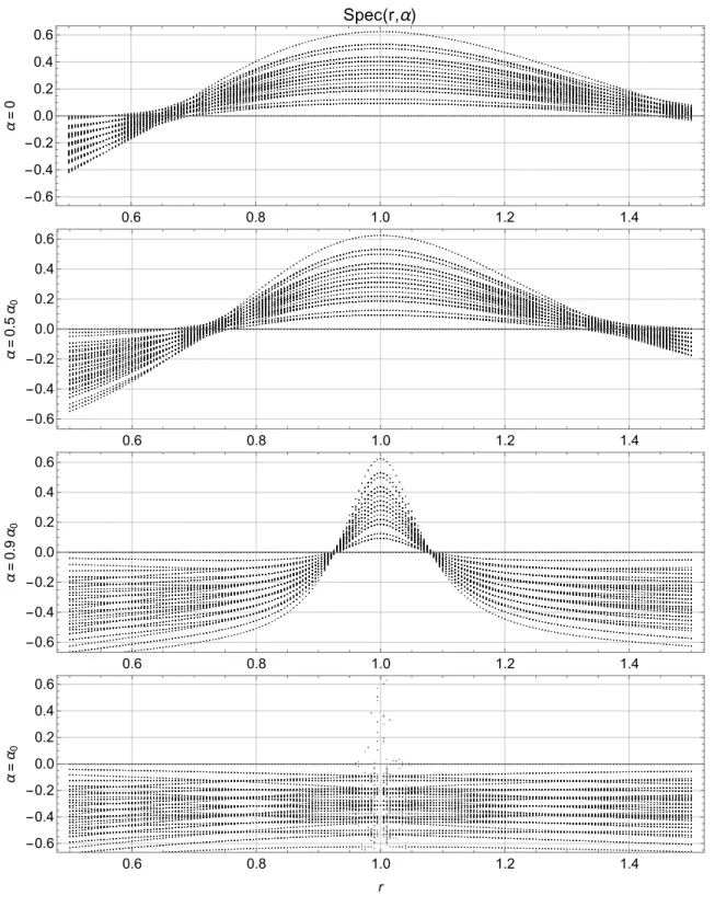
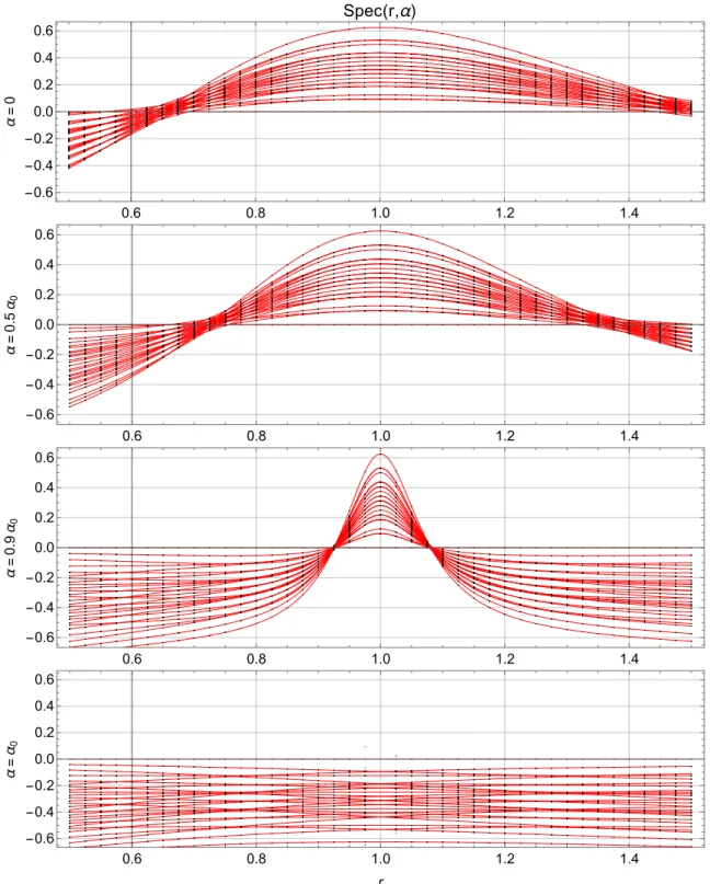
erklären, wie das Spektrum hierfür gefunden wurde. Dieses wird analysiert und sein
Kontinuumslimes wird bestimmt. Hierbei zeigt sich, dass dieses System nur dann kritisch
ist, wenn ausschließlich einer der beiden Parameter variiert werden darf.
Abstract
Phase transitions of second order play an important role in solid state physics. It is in their nature that they occur only in systems that are composed from an infinite number of components since, only that way, the necessary conditions for this (for example, scale invariance) are granted. Such a system at a second order phase transition is called critical.
The infinite number of particles poses a particular challenge, even for the description of classical systems. Quantum mechanical systems, however, are distinctly more difficult to treat in this context, since the dimension of their state space grows exponentially with the number of their particles, not to mention the fact that only a few – and usually only one-dimensional – quantum systems are exactly solvable. One of these exactly solvable one-dimensional quantum systems is the SU ( N ) Haldane-Shastry spin chain that may be regarded as the archetype of long-range spin chains. Moreover, it is critical in the continuum limit and its effective low-energy theory is the so-called SU ( N )
1Wess-Zumino- Witten model. It is a quantum field theory which is not only conformally invariant, so, in particular, scale invariant, but, furthermore, exhibits additional symmetry in the shape of an infinite extension of the Lie algebra su ( N ) associated with SU ( N ) . Recent studies show that, from these very structures of the SU ( N )
1WZW model, one can, in turn, derive spin systems, whose arrangement is not necessarily the one of a spin chain, but even two-dimensional distributions of the spins in the plane are possible. These systems are again characterized by long-range interactions, comparable to those of the Haldane-Shastry spin chain, which is also obtained as a result of an appropriate choice of parameters.
In this thesis, we extend the construction already known for the SU ( N ) case to the supersymmetric case of GL ( m | n ) . Here, we construct explicitly both, a special quantum state as well as a Hamiltonian that projects this quantum state to zero. We also discuss the Hamiltonian in the special case of the GL ( 1 | 1 ) spin chain and compare it to the respective GL ( 1 | 1 ) Haldane-Shastry spin chain on a bipartite state space. Both are critical and we identify the corresponding conformal field theories. Subsequently, we describe a general- ization of this system in terms of two parameters and explain how its spectrum was found.
It is then analyzed and its continuum limit is determined. In doing so, it shows that the system displays criticality only for generic values of one of the two parameters.
vi
Contents
1 Setting the Stage 1
1.1 The General Idea . . . . 2
1.1.1 Constructing the Hamiltonian . . . . 2
1.1.2 The SU ( 2 )
1WZW Model and the Haldane-Shastry Spin Chain . . . . 3
1.2 The Structure of this Thesis . . . . 5
2 Prerequisites 7
2.1 Some Super Structure . . . . 7
2.1.1 Basic Notions in Super Linear Algebra . . . . 7
2.1.2 The Superalgebra End (V ) . . . . 8
2.1.3 The Lie Superalgebra gl ( m | n ) and Its Defining Representation . . . . 9
2.1.4 Some gl ( m | n ) Representations and Their Tensor Products . . . . 11
2.2 The Pure Haldane-Shastry Chain for gl ( 1 | 1 ) -Spins . . . . 15
2.2.1 Diagonalization of the Hamiltonian . . . . 16
3 Construction of a
GL ( m | n )
-invariant Quantum Superspin System 253.1 Modus Operandi . . . . 26
3.2 The GL ( m | n ) WZW Model, Free Fields and Null Fields . . . . 30
3.3 Projection Operators onto Null Fields . . . . 33
3.4 The Derivation of the Hamiltonian . . . . 36
3.5 Simplification of the General Hamiltonian . . . . 41
3.6 Special Choices of m and n for GL ( m | n ) . . . . 44
3.6.1 Excluding fermions: M = n = 0 . . . . 44
3.6.2 Superdimension N = 1 . . . . 45
3.6.3 Superdimension N < 0 . . . . 46
3.6.4 Superdimension N = 0 . . . . 46
3.7 A Special Setup . . . . 47
3.8 The Seed State . . . . 51
3.8.1 General Properties . . . . 51
3.8.2 Free Field Correlator . . . . 52
4 The Uniform One-Dimensional Setup of Alternating
gl ( 1 | 1 )
-Spins 574.1 The Alternating Haldane-Shastry Model for gl ( 1 | 1 ) -Spins . . . . 58
4.2 The One-Dimensional Alternating Setup for gl ( 1 | 1 ) . . . . 68
4.3 Connecting the Ising CFT to a Logarithmic CFT . . . . 71
4.4 Proposing a Regularization Scheme for Haldane-Shastry Spin Chains – or
How To Get The Scaling Right . . . . 74
4.4.1 The Central Charge of the SU ( 2 ) Haldane-Shastry Spin Chain . . . . 74
4.4.2 The Central Charge of the SU ( N ) Haldane-Shastry Spin Chain . . . 78
4.4.3 The Central Charge of the GL ( 1 | 1 ) Haldane-Shastry Spin Chains . . 81
5 The Two-Parameter Spin Ladder 83
5.1 The Setup . . . . 84
5.2 The gl ( m | m ) -Spin Ladder . . . . 86
5.3 The gl ( 1 | 1 ) -Spin Ladder . . . . 87
5.3.1 Establishing Analytic Expressions for the Full Spectrum . . . . 88
5.3.2 Analytic Discussion of the One-Particle Energies . . . . 95
5.3.3 A Guess on the Hamiltonian . . . 102
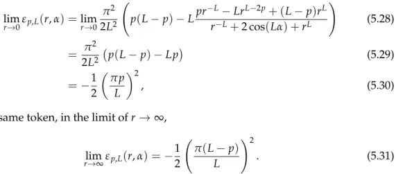
5.3.4 The Continuum Limit . . . 103
6 Conclusion and Outlook 111
Bibliography 115
viii
1
Setting the Stage
Not how the world is, but that it is, is the mystery.
– Ludwig Wittgenstein Even though the foundations of quantum mechanics date back about 100 years and much progress concerning theoretical developments has been made in the field, actual calcula- tions even in low-dimensional quantum mechanical systems are exceedingly costly and difficult when increasing the system size L. The reason for this is that the Hilbert space of such a system grows exponentially with L.
In order to tackle this problem, many useful tools have been developed. Some more general ones aim at implementing efficient algorithms for exact diagonalization of the Hamiltonian describing the system at hand.
Restricting the number of dimensions to just one, very special techniques can be em- ployed if the system is fully integrable and can, thus, be solved analytically. Even though this may sound simple, it involves the use of a huge machinery, e.g. Bethe ansatz [1] and more refined version of the same.
In some more general one-dimensional cases, the part of the states whose entropy obeys an area law can be approximated through a matrix product state (MPS) [2]. Let the Hilbert space H be given by H = V
⊗Lwith an orthonormal basis (ONB) {| i i}
i=1,...,don V . An ONB on H is then given by the set of all combinations of the form | i
1. . . i
Li : = ∏
Lj=1| i
ji . The MPS interpolates between a product state without entanglement
| Ψ
classicali =
∑
d i1,...,iL=1A
[i1]1
· · · A
[iLL]| i
1. . . i
Li , (1.1) described by d · L coefficients, and a possibly fully entangled quantum state
| Ψ
fully entangledi =
∑
d i1,...,iL=1C
i1...iL| i
1. . . i
Li , (1.2)
described by d
Lcoefficients, where d is the dimensionality of the on-site Hilbert spaces V .
An MPS is fully described by D
2· d · L coefficients where D is an integer quantifying the
1 Setting the Stage
dimension of certain matrices that belong to these on-site Hilbert spaces:
| Ψ
MPSi =
∑
d i1,...,iL∑
D α,...,δA
[i1]1,(αβ)
· A
[i2]2,(βγ)
· · · A
[iL]L,(δα)
| i
1. . . i
Li . (1.3) The bond dimension D can be tuned in order to reach the desired compromise between precision and convenience. The important observation here is that the necessary amount of information is linear in system size L.
Nevertheless, systems at criticality, in principle, become impossible to handle in this fashion as the bond dimension D of the MPS scales exponentially in L [3].
A possible way to solve this problem is the use of an infinite-dimensional matrix product state (IMPS) which is a generalization of the MPS through the use of chiral vertex operators from a two-dimensional conformal field theory (CFT). As it makes use of operator valued field insertions φ ( z
j) instead of matrices A
[ij]j,(αβ)
, it evades the limitation of a finite bond dimension D. Inspired by Moore and Read [4], one such construction was proposed by Cirac and Sierra in [5] in order to approximate ground state wave functions of spin chains that, in particular, can become critical for certain values of their parameters, e.g. the XXZ spin chain. This idea will be explained in the next Section.
1.1 The General Idea
As just mentioned, an IMPS will take the form
| Ψ
IMPS( z
1, . . . , z
L)i =
∑
d i1,...,iL=1h φ
i1( z
1) · · · φ
iL( z
L)i | i
1. . . i
Li , (1.4) by analogy with eq. (1.3), where z
jsimply parametrizes the location of sites j in the complex plane. However, now the coefficients of the expansion in the usual basis | i
1. . . i
Li are computed by finding the vacuum expectation value (instead of taking the trace) of the product of L chiral fields φ ( z
j) (instead of matrices) that belong to representations of certain algebras of two-dimensional CFTs and that fulfill model specific operator product expansions (OPE). In CFT, the object ψ ({ z
m}) : = h φ ( z
1) · · · φ ( z
L)i is called a chiral correlator and it can, in principle, be calculated analytically from the OPE.
In [6], Nielsen, Cirac and Sierra have proposed an interesting construction for finding a parent Hamiltonian whose ground state is given by eq. (1.4).
1.1.1 Constructing the Hamiltonian
Their key observation was the existence of null states χ ( z ) in representations of CFTs (e.g.
the SU ( 2 )
kWZW model in their paper [6]). Since χ ( z ) decouples from the rest of the module
0 ≡ h φ ( z
1) · · · χ ( z
i) · · · φ ( z
L)i , (1.5)
2
1.1 The General Idea
SU ( 2 )
1WZW z
iz
jr
ijcontinuum limit
lattice regularization SU ( 2 ) Haldane-
Shastry
Figure 1.1: The correspondence between the SU(2)Haldane-Shastry spin chain and the SU(2)WZW model at levelk=1.
they are called null states. However, they can be traced back to the primary states φ ( z ) and thus the identity eq. (1.5) can be rewritten as
0 = P
i({ z
j})h φ ( z
1) · · · φ ( z
i) · · · φ ( z
L)i (1.6) where P
i({ z
j}) is an operator carrying one adjoint index
1(for simplicity of notation hidden at this point) of the global symmetry, acting on the full chiral correlator and, obviously, annihilating it. Repeating the same procedure with all of the field insertion at all points z
j, we find L such operators P
j, all of them annihilating the chiral correlator. To this end, we compute
H : =
∑
L i=1H
i: =
∑
L i=1(P
i)
†P
i(1.7)
which is hermitian, positive semi-definite, commutes with the global symmetry and annihi- lates the chiral correlator. Therefore, H must be a parent Hamiltonian
2of the exact ground state given by eq. (1.4), which is analytically computable.
1.1.2 The SU ( 2 )
1WZW Model and the Haldane-Shastry Spin Chain
Having proposed the previously sketched construction, the authors of [6] exemplarily calculated the ground state and parent Hamiltonian for the SU ( 2 )
1WZW model with field insertions φ ( z
j) distributed on the unit circle. What they found, is depicted in Figure 1.1.
Making use of the symmetries of the chiral part of the SU ( 2 )
1WZW model via this construc- tion, they obtained the Haldane-Shastry spin chain with spin-
12spins [7, 8], a generalization of the Heisenberg spin chain [9, 10], but with long-range interaction ∼ S
i· S
j/r
2ij. Vice versa,
1The construction is not limit to only one adjoint index. Depending, e.g. on the level of the WZW model, there can be more adjoint indices.
2The wordparentin this context indicates that one starts with the construction of a state and then derives a Hamiltonian associated with this state.
1 Setting the Stage
taking this Haldane-Shastry spin chain to the thermodynamic limit, it becomes critical and its low-energy spectrum can be analyzed using techniques called finite-size scaling [11, 12]:
This way, one can extract its conformal anomaly c = 1 and conformal dimensions h
i, and these match the data of the SU ( 2 )
1WZW model exactly. In this sense, one can refer to this construction as a discretization of the SU ( 2 )
1WZW model. In the meantime it has become clear that this correspondence also carries over to SU ( N ) [13, 14].
An immediate question is whether this holds for other symmetries, e.g. GL ( m | n ) . Also, and more generally, it seems worthwhile to treat the GL ( m | n ) WZW model in the same way as, e.g. gl ( 1 | 1 ) is related to supersymmetric quantum mechanics. Additionally, supersym- metry plays an important role for the description of disordered systems [15]. Furthermore, WZW models based on supergroups describe the physics of dilute polymers [16], critical systems with quenched disorder [17] and percolation [18]. Moreover, as mentioned in [19], most of the minimal unitary CFTs that have been solved so far are actually not suitable as an ad-hoc realistic description of critical systems in, e.g. condensed matter physics because only a few of them come with no more than the necessary operator content to describe system at hand making any fine-tuning superfluous. On the other hand, it has become clear that many systems of statistical physics are, in a way, nonlocal in character with their observables, such as critical exponents, rather belonging to non-unitary CFTs with conformal anomaly c = 0 and, hence, described by a Hamiltonian which is not hermitian.
Further, it is also expected that the two-dimensional sigma model on a super-coset space associated with the plateaux transition in the integer quantum Hall effect [15, 20–22] flows to a strongly interacting CFT with central charge zero [23]. Therein, it is also mentioned that this system can be mapped to a Heisenberg-like superspin chain of specific alternating infinite-dimensional gl ( 2 | 2 ) representations that were first identified by Read (cf. reference [47] in [23], private communication between the authors). Until now, however, there exists no solution for these spin chains and, hence, no idea about their thermodynamic limit and little is known about the governing CFT. However, also therein, the hope was articulated that a deformation of this spin chain to a Haldane-Shastry-like spin chain would enhance the symmetry of the spin chain in order to be able to diagonalize it and constrain its critical behavior.
The general idea for the construction of spin chain Hamiltonians from CFT put forward by Nielsen, Cirac and Sierra might prove powerful enough to shed some light on this matter because it allows for the construction of various spin systems (on two-dimensional or one-dimensional lattices, regular or irregular, and, in particular, Haldane-Shastry-like spin chains) from any CFT that features null states. One can then hope for such a spin system of Haldane-Shastry-type to be critical and to disclose some information about the CFT it is described by. It will be shown in this thesis that this is the case for a system of alternating fundamental and antifundamental gl ( 1 | 1 ) -spins. Additionally as this case shows, these Haldane-Shastry-like spin chains seem to capture the properties of the CFT particularly well since their dispersion relation are given by the simplest relation capable of exhibiting relativistic behavior in the low-energy regime (i.e. ε
p∼ p ( π − p ) with p the momentum of an excitation) while the dispersion relation of its Heisenberg version,
4
1.2 The Structure of this Thesis
covered in [24], is given by a transcendental function, ε
p∼ sin p. Also, as explained in [25] and going in the same vein, due to its specific long-range interaction, the Haldane- Shastry model exactly follows the scaling of the CFT, even at finite system size whereas spin chains like the Heisenberg chain come with logarithmic corrections as a result of the long-wavelength corrections depending on the system size. The reason for this particularly nice property of the Haldane-Shastry model is its Yangian symmetry [26]. Thus, it appears to be not too farfetched to hope to encounter a similarly well-behaved structure in the Haldane-Shastry-like spin chains that can be constructed from non-unitary CFTs following the idea of Nielsen, Cirac and Sierra.
1.2 The Structure of this Thesis
The construction of the superspin systems will require some preparation. Thus, in the next Chapter, some necessary concepts from super linear algebra and Lie superalgebras and some of their representations will be introduced. However, this will be kept to a minimum, mainly fixing notation. Chapter 2 concludes with a basic discussion of the GL ( 1 | 1 ) Haldane-Shastry model since we will encounter the GL ( 1 | 1 ) Haldane-Shastry model again in later Chapters. In [27], it was shown to be a model of non-interacting fermions and, hence, exactly solvable. In the continuum limit, it turns out to be of the same structure as the disorder sector of the Ising CFT [28].
Systems of gl ( m | n ) -superspins with long-range interactions, arbitrarily distributable in the complex plane, will be constructed in Chapter 3. The necessary ingredients from CFT will be introduced along the way. In this affair, an important ingredient will be the concept of a null state. The null states will allow us to construct a singlet wave function from particular CFT correlation functions (i.e. chiral correlators) and projection operators which project this singlet to zero. Further, the projection operators can be combined to form an operator, which will be used as the Hamiltonian of the system. The way it is constructed, the system will possess global GL ( m | n ) -invariance and long-range interactions between up to three individual spins.
3Then, we will comment on some special cases for the choice of m and n as well as for a Haldane-Shastry-like distribution of the spins for m = n. This Chapter concludes with the analytic calculation of the singlet wave function from the CFT correlators for arbitrary m and n and distribution of the spins in the complex plane.
As the Hamiltonian becomes particularly simple for m = n for spins uniformly dis- tributed on the unit circle, Chapter 4 is dedicated to the discussion of these kinds of models.
However, for its similarity with the alternating Haldane-Shastry model of gl ( 1 | 1 ) -spins, we will first solve this model before fleshing out our Hamiltonian. In both cases, we will shed light on their thermodynamic limit in order to eventually see some surprising interrelation emerge: Both have c = − 2, contrary to the central charge c = 0 of the GL ( 1 | 1 ) WZW model which has been discussed and solved in [29]. However, they are not described by
3As a manifestation of the monogamy of entanglement, this can also be expressed as the product of two spin-spin interactions with one common spin.
1 Setting the Stage
the same CFT as we will see. Furthermore, in the analysis of these systems, it appears that naïve finite-size scaling of the ground state energy leads to inconsistent results. The root of this seems to be that the range of summation in the definition of the long-range Haldane-Shastry spin chains must be slightly altered in order to be in perfect analogy with the energy operator L
0stemming from the Sugawara construction of the WZW model.
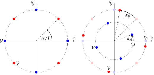
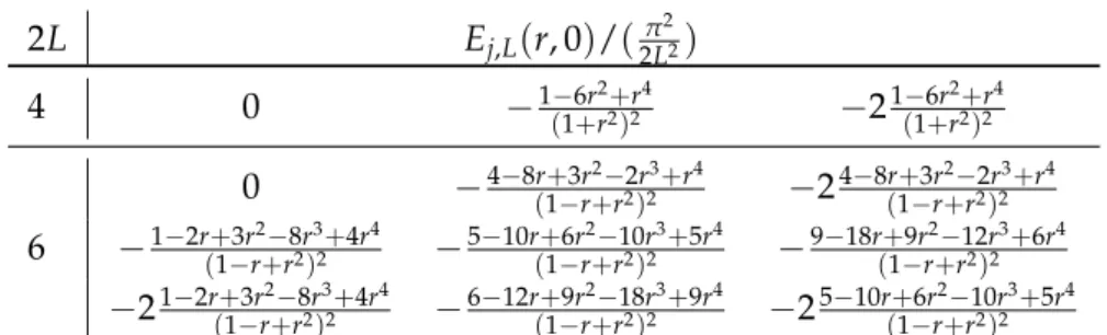
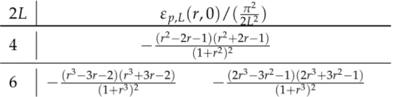
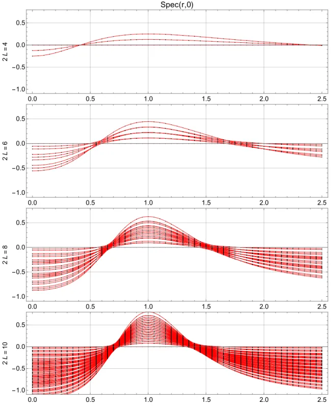
In Chapter 5, we will first describe a gl ( m | n ) -spin ladder setup on a bipartite lattice built from the fundamental representation V and its dual ¯ V . It has two parameters, one angular (α), the other radial (r). We will then restrict ourselves to the case m = n and give the GL ( m | m ) Hamiltonian from our construction in terms of r and α. Then, we will propose an exact analytic expression for the full spectrum of the gl ( 1 | 1 ) -spin ladder, including its full r- and α-dependence and explain how this was found. With these solutions at hand, we discuss the continuum limit of the generic gl ( 1 | 1 ) -spin ladder at any admissible value of r and α and infer that the gl ( 1 | 1 ) -spin ladder is only critical for one particular value of r.
The final Chapter will present a summary of all the results and close with some conclud- ing remarks and an outlook.
6
2
Prerequisites
If you are lost, find where you’re at.
– Róisín Murphy, Where Is The What If The What Is In Why?
In this preliminary Chapter, we will introduce the super structures that we will need for the following construction of the superspin systems and recap the discussion of the Haldane-Shastry model of gl ( 1 | 1 ) -superspins.
2.1 Some Super Structure
In this thesis, quantum superspin systems are constructed from CFT. These superspins are associated with operators that act on a Z
2-graded vector space which we will denote by V or ¯ V , depending on its transformation properties under some symmetry described in Section 2.1.3.
In the following Sections, we will recite some basics of the structures that will be necessary for the construction of the superspin systems in Chapter 3. A very nice introduction to the topic can be found in [30], for specific information on Lie superalgebras, one can consult [31] and a broader introduction to the topic of supersymmetry from a mathematical perspective is presented in [32].
2.1.1 Basic Notions in Super Linear Algebra We start from a complex Z
2-graded vector space
V = V
0⊕ V
1. (2.1)
The first direct summand V
0contains all elements that are called even (or bosonic) and the
second summand V
1contains all odd (or fermionic) elements. Here and in what follows,
we concentrate on the particular case of V = C
m|n. Its basis elements shall be denoted by
e
awith a = 1, 2, . . . , m + n. The grading is a map | • | sending a homogeneous (meaning
either strictly even or odd) element to the elements 0 (even) or 1 (odd) of Z
2understood as
a field so that they can be added and multiplied. We will always assume a homogeneous
2 Prerequisites
basis { e
a}
a, so that we have
| e
a| =
0 if 1 ≤ a ≤ m,
1 if m + 1 ≤ a ≤ m + n.
(2.2)
By abuse of notation, we will treat | e
a| and | a | as meaning the same. Also, we will often write a in exponents of (− 1 ) instead of | a | . This should not lead to any confusion, though.
Next, we define the dual vector space of V , ¯ V , that consists of all linear functionals mapping any element of V to the complex numbers. We define a homogeneous basis { e
b}
bon ¯ V by each element’s action on any basis element e
c:
e
b( e
c) : = δ
bc. (2.3)
By linearity, this extends to all elements of V and ¯ V . With this definition and due to the in supermathematics omnipresent Koszul sign rule, we have on the other hand
e
c( e
b) = δ
cb(− 1 )
cb= δ
bc(− 1 )
b, (2.4) leading to a sign change if and only if we pass an odd element by another odd element.
Also, by the last equality, it is evident that we silently used the same grading for e
bas given in eq. (2.2).
2.1.2 The Superalgebra End (V )
Armed with this much, we may define the space of linear maps from V to itself, End (V ) : The basic result from usual linear algebra carries over to the super case, i.e.
End (V ) : = V ⊗ V ¯ . (2.5)
As such, it is a graded vector space itself and the canonical (homogeneous) basis is given by the set { E
ab: = e
a⊗ e
b}
a,b=1,...,m+n. Their degree is defined in terms of the grading on V and ¯ V :
| e
a⊗ e
b| = | e
a| + | e
b| . (2.6) From the choice of ¯ V , it is also clear how such a basis element E
abacts on a basis element e
c∈ V :
E
abe
c= e
aδ
bc. (2.7)
Again, this extends to all elements in End (V ) and V by linearity. Furthermore, we can concatenate two maps,
E
dfE
abe
c= E
dfe
aδ
cb= e
dδ
afδ
cb, (2.8)
8
2.1 Some Super Structure
which defines a product in End (V ) :
E
dfE
ab= E
dbδ
af. (2.9)
This turns End (V ) into an algebra with consistent grading, i.e.
| E
dfE
ab| = | E
df| + | E
ab| δ
af= ( d + f + a + b ) δ
af= ( d + b ) δ
af(2.10)
= | E
db| δ
af(2.11)
and, hence, into what is called a superalgebra. Not to our surprise, End (V ) is also associa- tive:
E
gh( E
dfE
ab) = E
ghE
dbδ
af= E
gbδ
hdδ
af= E
gfE
abδ
dh= ( E
ghE
df) E
ab. (2.12) Finally, in analogy with the classical case, End (V ) is isomorphic to the associative algebra of all ( m | n ) × ( m | n ) matrices with entries in C. Their basic structure is such that they have two even blocks, one of them m × m-dimensional and the other n × n-dimensional, along their diagonal and two odd blocks, m × n-dimensional and n × m-dimensional, on the off-diagonal. A homogeneous matrix of this form has only entries either on the even or the odd blocks in C. It is then even or, respectively, odd. Furthermore, the supertrace of such a matrix is defined as the trace of the first even block (m × m-dimensional) minus the trace of the second even block (n × n-dimensional). Thus, the definition of the supertrace also carries over to elements of End (V ) . In particular, we find for the supertrace of the identity element of End (V )
str I = str E
aa=
∑
m a=11 −
m+n a=
∑
m+11 = m − n = : N. (2.13)
The quantity N is also referred to as the superdimension of V , sdim V . These are the necessary ingredients from super linear algebra for what follows.
2.1.3 The Lie Superalgebra gl ( m | n ) and Its Defining Representation
Just as in the classical case, any associative superalgebra can be turned into a Lie super- algebra. We will only deal with the Lie superalgebra gl ( m | n ) constructed from End (V ) , however, there is a variety of other complex finite-dimensional Lie superalgebras. They have been constructed and classified by Kac in [33, 34].
We start by defining a Lie bracket for the basis elements of End (V ) consistent with the Koszul sign rule,
[ E
ab, E
cd] : = E
abE
cd− (− 1 )
|Eab||Ecd|E
cdE
ab, (2.14)
and compatible with the grading. This extends to all elements of End (V ) and defines the
2 Prerequisites
product of the Lie superalgebra associated with End (V ) :
gl ( m | n ) : = { End (V ) , [• , •]} . (2.15) The bracket of the Lie superalgebra gl ( m | n ) is anti-supersymmetric,
[ X, Y ] = −(− 1 )
|X||Y|[ Y, X ] , (2.16) and respects the graded Jacobi-identity,
[ X, [ Y, Z ]](− 1 )
|X||Z|+ [ Y, [ Z, X ]](− 1 )
|Y||X|+ [ Z, [ X, Y ]](− 1 )
|Z||Y|= 0, (2.17) for any choice of homogeneous elements X, Y, and Z in gl ( m | n ) .
Next, we would like to define an invariant bilinear form. The natural choice in the classical case is the Killing form, which, in the super case, turns out to be nondegenerate only for m 6= n, and, zero when m = n. Since this case is of particular interest for our discussion in Chapters 4 and 5, instead of taking the supertrace in the adjoint representation, we, thus, resort to taking the supertrace in the fundamental representation,
κ ( E
ab, E
cd) : = str ( E
abE
cd) = δ
cbstr ( E
ad) = δ
bcδ
da(− 1 )
a, (2.18) again, extended to gl ( m | n ) by bilinearity. For later purposes, we will also write
κ
a cb,d: = κ ( E
ab, E
cd) = δ
daδ
bc(− 1 )
a. (2.19) It turns out to be consistent,
κ ( X, Y ) = 0 for all homogeneous X and Y with | X | 6= | Y | , (2.20) supersymmetric,
κ ( X, Y ) = (− 1 )
|X||Y|κ ( Y, X ) , (2.21) and invariant,
κ ( X, [ Y, Z ]) = κ ([ X, Y ] , Z ) , (2.22) and, in addition, nondegenerate,
(∀ Y ∈ gl ( m | n ) : κ ( X, Y ) = 0 ) ⇒ X = 0. (2.23) With this invariant bilinear form, we can now define the quadratic Casimir for some representation ρ of gl ( m | n ) ,
C : = ρ ( E
ab) ρ ( E
ba))(− 1 )
b. (2.24) For the fundamental representation, ρ
V( E
ab) = E
ab, with representation space V = V , we
10
2.1 Some Super Structure
find
C
V: = E
abE
ba(− 1 )
b= ( m − n ) E
aa= N I. (2.25) The antifundamental representation is defined by the action of the E
abon ¯ V which is defined via the relation to V . Therefore we calculate
E
ab· e
c( e
d) = −(− 1 )
c(a+b)e
c( E
abe
d) = −(− 1 )
c(a+b)e
c( e
a) δ
db(2.26)
= −(− 1 )
a+abδ
cae
b( e
d) (2.27) which implies ρ
V¯( E
ab) = −(− 1 )
abE
bawith E
ba: = e
b⊗ e
aand keeping in mind the conse- quences of the Koszul sign rule as given in eq. (2.4), e
a( e
c) = δ
ca(− 1 )
awhile the overall sign change stems from turning the right module into a left module. With this, we compute the quadratic Casimir in the antifundamental representation and find
C
V¯· e
c: = (− 1 )
bρ
V¯( E
ab) ρ
V¯( E
ba) e
c= −(− 1 )
b+baρ
V¯( E
ab) E
abe
c(2.28)
= −(− 1 )
b+baρ
V¯( E
ab) e
a⊗ e
b( e
c) = −(− 1 )
baρ
V¯( E
ab) e
aδ
cb(2.29)
= E
bae
aδ
cb= e
b⊗ e
a( e
a) δ
cb= e
bδ
aa(− 1 )
aδ
bc(2.30)
= e
cN (2.31)
which is equivalent to the result for the fundamental representation V .
2.1.4 Some gl ( m | n ) Representations and Their Tensor Products
In the preceding Section, we have already learned about the fundamental and antifunda- mental representation, ρ
Vand ρ
V¯, both of which are irreducible gl ( m | n ) representations.
Due to the way gl ( m | n ) is constructed from V , ρ
Vis also referred to as the defining rep- resentation. However, making the distinction between ρ
Vand ρ
V¯is simply a matter of convention. Moreover, the systems to be constructed in Chapter 3 will be invariant under the exchange of these, i.e. under parity. In order to describe interactions between different superspins
1meaning different representations, we will also need tensor products consisting of a choice of up to three representations. Generalizing the quadratic Casimir to those tensor products helps to find their decomposition. Nevertheless, we will see that there is a caveat: While V and ¯ V are irreducible, we will also encounter reducible but indecom- posable representations. This means that they have a proper gl ( m | n ) -submodule but it is not possible to recast the indecomposable representation as a direct sum of such proper gl ( m | n ) -submodules. For a general discussion of tensor products for gl ( m | n ) , [35] can be consulted.
1We will also refer to them simply asspins.
2 Prerequisites
Twofold Tensor Products from
V
andV ¯
For computing the decomposition of V ⊗ V , we have to define how the quadratic Casimir acts on it. This boils down to defining a coproduct ∆ and fixing
∆ ( C ) e
a⊗ e
b= ( C
V· e
a) ⊗ e
b+ ∑
c,d
(− 1 )
d+a(d+c)E
cde
a⊗ E
dce
b(2.32) +(− 1 )
d+(c+d)+a(c+d)E
dce
a⊗ E
cde
b+ e
a⊗ ( C
V· e
b) (2.33) which simplifies to
∆ ( C ) e
a⊗ e
b= 2 N e
a⊗ e
b+ (− 1 )
abe
b⊗ e
a. (2.34)
From this, one can infer that V ⊗ V decomposes into a symmetric and an antisymmetric representation,
V ⊗ V = S + A , (2.35)
which are spanned by e
a⊗ e
b+ (− 1 )
abe
b⊗ e
aand e
a⊗ e
b− (− 1 )
abe
b⊗ e
a, respectively, with Casimir eigenvalue 2 ( N + 1 ) and 2 ( N − 1 ) , respectively. An analogous result holds for V ⊗ ¯ V ¯ .
Next, we find the action of the Casimir on the elements e
a⊗ e
bin the mixed tensor product V ⊗ V ¯ :
∆ ( C ) e
a⊗ e
b= ( C
V· e
a) ⊗ e
b+ ∑
c,d
−(− 1 )
d+a(d+c)E
cde
a⊗ E
dc· e
b(2.36)
−(− 1 )
d+(c+d)+a(c+d)E
dce
a⊗ E
cd· e
b+ e
a⊗ ( C
V¯· e
b)
= 2 N e
a⊗ e
b− δ
ba(− 1 )
a∑
c
e
c⊗ e
c!
(2.37)
=
2N e
a⊗ e
bif a 6= b, 2 ( N e
a⊗ e
a− ∑
ce
c⊗ e
c) if a = b ≤ m, 2 ( N e
a⊗ e
a+ ∑
ce
c⊗ e
c) if a = b > m.
(2.38)
For N 6= 0 (implying m 6= n), we, obviously, have one submodule spanned, e.g., by { e
a⊗ e
b}
a6=b, { e
a⊗ e
a− e
a+1⊗ e
a+1}
a=1,...,m−1, { e
a⊗ e
a− e
a+1⊗ e
a+1}
a=m+1,...,m+n−1and e
1⊗ e
1+ e
m+1⊗ e
m+1, with Casimir eigenvalue 2N and another one-dimensional submodule spanned by ∑
ae
a⊗ e
awith Casimir zero. However, this decomposition breaks down if we
12
2.1 Some Super Structure
choose N = 0: In this case, the Casimir is non-diagonalizable,
∆ ( C ) e
a⊗ e
b=
0 if a 6= b,
− 2 ∑
ce
c⊗ e
cif a = b ≤ m, 2 ∑
ce
c⊗ e
cif a = b > m.
(2.39)
While we still find the one-dimensional invariant submodule spanned by ∑
ae
a⊗ e
awith eigenvalue zero, it does not decouple from the rest of the tensor product as any state e
a⊗ e
ais mapped onto it. Therefore, the mixed tensor product V ⊗ V ¯ is reducible but indecomposable if the superdimension N vanishes.
Threefold Tensor Products from
V
andV ¯
The threefold tensor products are relevant for us because we will need the tensor product of the adjoint representation with representation space J = V ⊗ V ¯ with the fundamental (and antifundamental, respectively):
J ⊗ V = V ⊗ V ⊗ V ¯ . (2.40) For the action of the quadratic Casimir on the product basis { e
a⊗ e
b⊗ e
c}
a,b,c∈{1,...,p}, we have
2∆
2( C ) e
a⊗ e
b⊗ e
c= ∑
d,f
(− 1 )
f∆ ( E
df) ∆ ( E
fd) e
a⊗ e
b⊗ e
c(2.41) which, after a lengthy calculation, yields
∆
2( C ) e
a⊗ e
b⊗ e
c= 3N e
a⊗ e
b⊗ e
c+ 2 (− 1 )
ab+bc+cae
c⊗ e
b⊗ e
a(2.42)
− 2 (− 1 )
aδ
ba∑
d
e
d⊗ e
d⊗ e
c− 2δ
bc∑
d
(− 1 )
de
a⊗ e
d⊗ e
d. We will see that the eigenvalues of the quadratic Casimir are N, 3N − 2 and 3N + 2.
Let us first define the 2p vectors u
c: = ∑
ae
a⊗ e
a⊗ e
cand v
a: = ∑
b(− 1 )
be
a⊗ e
b⊗ e
beach of them spanning a submodule isomorphic to V (unless N = ± 1 in which case the Casimir will, obviously, not resolve its eigenvectors with eigenvalue N and 3N ∓ 2):
∆
2( C ) u
c= N u
c, (2.43)
∆
2( C ) v
c= N v
c. (2.44)
Both sets of these vectors are, of course, in the span of states spanning the whole tensor
2For clarity, we will, in this Section, indicate summation over double indices explicitly through the summation sign∑in order to prevent confusion.
2 Prerequisites
product. These states can be recast into new basis vectors,
w
±a cb: = e
a⊗ e
b⊗ e
c± (− 1 )
ab+bc+cae
c⊗ e
b⊗ e
a, (2.45) and they are useful for forming linear combinations together with the w
±a cbthat will feature an eigenvalue of 3N − 2 or 3N + 2. In the simplest case, a arbitrary, b ∈ { / a } , c ∈ { / a, b } , this is not even necessary:
∆
2( C ) w
±a cb= ( 3N ± 2 ) w
±a cb. (2.46) As a matter of fact, the u
cand v
care obviously linearly independent from these p ( p − 1 )( p − 2 ) vectors. The same is true for the p ( p − 1 ) non-zero
3cases a = c, b ∈ { / a } :
∆
2( C ) w
(−1)aa ab= 3N + (− 1 )
a2 w
(−1)aa ab. (2.47) In the remaining 2p ( p − 1 ) + p cases, w
±a ca(c 6= a) and w
(−1)aa aa4
on the one hand and u
cand v
con the other are not linearly independent and the ws are not in general eigenvectors of the Quadratic Casimir. In the latter cases, we find
∆
2( C ) w
(−1)aa aa= 3N + (− 1 )
a2 w
(−1)aa aa− 1 + (− 1 )
a2 ( u
a+ v
a) , (2.48) which are eigenvectors only for odd a, so with eigenvalue 3N − 2. For even a, it can be calculated that, in order to decouple the ( 3N + 2 ) -part from 2 ( u
a+ v
a) , we have to form a new linear combination,
∆
2( C )
w
+a aa− 1
N + 1 ( u
a+ v
a)
= ( 3N + 2 )
w
+a aa− 1
N + 1 ( u
a+ v
a)
, (2.49) which is possible unless N = − 1: In that case, w
+a aaand 2 ( u
a+ v
a) form an indecom- posable Jordan block. An analogous procedure yields for the 2p ( p − 1 ) cases w
±a cawith c 6= a,
∆
2( C ) w
±a ca− (− 1 )
aN ± 1 ( u
c± v
c)
!
= ( 3N ± 2 ) w
±a ca− (− 1 )
aN ± 1 ( u
c± v
c)
!
, (2.50) which again fails for those states with eigenvalue 3N ± 2 unless N 6= ∓ 1. This failure is an important hint for the construction of the projection operator P
ithat will be used in order to construct the GL ( m | n ) -symmetric Hamiltonian: P
iwill be constructed such that it certainly projects out all parts in the threefold tensor product V ⊗ V ⊗ V ¯ associated to the fundamental representation V (the antifundamental representation ¯ V , respectively)
3Obviously, we havew−(−1)aa ab ≡0.
4Again, we havew−(−1)aa aa ≡0.
14
2.2 The Pure Haldane-Shastry Chain for gl ( 1 | 1 ) -Spins as the desired null states to project onto for sure are not associated to the fundamental representation.
As a consequence, for positive N, P
iwill project onto the submodule of eigenvalue 3N + 2 so that the indecomposability between the subspace with eigenvalue 3N − 2 and the subspaces with eigenvalue N in case N = 1 will play no role as they are collectively projected out. For the analogous reason, for negative N, P
iwill project onto the submodule of eigenvalue 3N − 2, so that the indecomposability between states with eigenvalue N and 3N + 2 for N = − 1 does no harm.
To sum up, the threefold tensor product we are interested in yields
J ⊗ V = N ⊕ X (2.51)
with N being defined as the submodule with
∆
2( C ) N = 3N + sgn ( N ) 2
N (2.52)
and X the span of all other states (with eigenvalues N or 3N − sgn ( N ) 2 within J ⊗ V ) whose decomposition is irrelevant to us as X will be projected out by P
i.
2.2 The Pure Haldane-Shastry Chain for gl ( 1 | 1 ) -Spins
In his monograph [36], Greiter gives the Hamiltonian for the Haldane-Shastry model as H
HS=
2π L
2 L−1 k>∑
j=0S
j· S
k| η
j− η
k|
2with η
j: = exp
j 2πi L
. (2.53)
Using | exp ( j
2πiL) − exp ( k
2πiL)|
2= 4 sin
2(j−k)π L
, we arrive at
H
HS= π
2
L
2L−1 j
∑
<kS
j· S
ksin
2(( j − k ) π/L ) , (2.54) so that, in the large L limit, the nearest-neighbor interaction becomes Heisenberg-like, which is one reason for the scale factor in front of the sum in eq. (2.53). Another reason is that, with this normalization, we can safely take the thermodynamic limit L → ∞. Now using the identity S
j· S
k=
12( P
jk−
12) for the su ( 2 ) -generators S
jin order to generalize this expression, we receive
H
HS= π
2
2L
2L−1 j