Some Evidence on the Relevance of the Chain-reaction Theory in Selected Countries

IHS Economics Series Working Paper 207

May 2007

Some Evidence on the Relevance of the Chain-reaction Theory in Selected Countries

Helmut Hofer

Robert M. Kunst

Wolfgang Schwarzbauer

Ulrich Schuh

Dennis J. Snower

Impressum Author(s):

Helmut Hofer, Robert M. Kunst, Wolfgang Schwarzbauer, Ulrich Schuh, Dennis J.

Snower Title:

Some Evidence on the Relevance of the Chain-reaction Theory in Selected Countries ISSN: Unspecified

2007 Institut für Höhere Studien - Institute for Advanced Studies (IHS) Josefstädter Straße 39, A-1080 Wien

E-Mail: o ce@ihs.ac.atffi Web: ww w .ihs.ac. a t

All IHS Working Papers are available online: http://irihs. ihs. ac.at/view/ihs_series/

This paper is available for download without charge at:

https://irihs.ihs.ac.at/id/eprint/1768/

207 Reihe Ökonomie Economics Series

Some Evidence on the Relevance of the Chain-reaction Theory in Selected Countries

Helmut Hofer, Robert M. Kunst, Wolfgang Schwarzbauer,

Ulrich Schuh, Dennis J. Snower

207 Reihe Ökonomie Economics Series

Some Evidence on the Relevance of the Chain-reaction Theory in Selected Countries

Helmut Hofer, Robert M. Kunst, Wolfgang Schwarzbauer, Ulrich Schuh, Dennis J. Snower May 2007

Institut für Höhere Studien (IHS), Wien

Institute for Advanced Studies, Vienna

Contact:

Helmut Hofer : +43/1/599 91-251 email: hofer@ihs.ac.at Robert M. Kunst : +43/1/599 91-255 email: kunst@ihs.ac.at Wolfgang Schwarzbauer : +43/1/599 91-112 email: schwarzba@ihs.ac.at Ulrich Schuh

: +43/1/599 91-148 email: schuh@ihs.ac.at Dennis J. Snower

The Kiel Institute for the World Economy Düsternbrooker Weg 120

24105 Kiel, Germany : +49/431/8814-235

email: dennis.snower@ifw-kiel.de

Founded in 1963 by two prominent Austrians living in exile – the sociologist Paul F. Lazarsfeld and the economist Oskar Morgenstern – with the financial support from the Ford Foundation, the Austrian Federal Ministry of Education and the City of Vienna, the Institute for Advanced Studies (IHS) is the first institution for postgraduate education and research in economics and the social sciences in Austria.

The Economics Series presents research done at the Department of Economics and Finance and aims to share “work in progress” in a timely way before formal publication. As usual, authors bear full responsibility for the content of their contributions.

Das Institut für Höhere Studien (IHS) wurde im Jahr 1963 von zwei prominenten Exilösterreichern – dem Soziologen Paul F. Lazarsfeld und dem Ökonomen Oskar Morgenstern – mit Hilfe der Ford- Stiftung, des Österreichischen Bundesministeriums für Unterricht und der Stadt Wien gegründet und ist somit die erste nachuniversitäre Lehr- und Forschungsstätte für die Sozial- und Wirtschafts- wissenschaften in Österreich. Die Reihe Ökonomie bietet Einblick in die Forschungsarbeit der Abteilung für Ökonomie und Finanzwirtschaft und verfolgt das Ziel, abteilungsinterne Diskussionsbeiträge einer breiteren fachinternen Öffentlichkeit zugänglich zu machen. Die inhaltliche Verantwortung für die veröffentlichten Beiträge liegt bei den Autoren und Autorinnen.

Abstract

In this paper we challenge the traditional labour market view, which argues that unemployment is determined in the long-term by its equilibrium rate, which in turn is affected by permanent shocks of some exogenous variables. In our empirical approach we decompose the dynamics of employment and labour force into transitory and permanent components. We estimated a small labour market model using VAR techniques. By simulating the model we are able to quantify the relative importance of the permanent and transitory components for the movements of the unemployment rate in four countries (Austria, France, UK, and USA). We find that the transitory component has a significant impact on unemployment only in the US. In contrast to that the permanent component appear to influence unemployment significantly in all included countries. In combination with the observation that labour market dynamics differ between countries, this may have powerful policy implications.

Keywords

Unemployment, natural rate hypothesis, labour markets, employment, adjustment costs

JEL Classification

J32, J60, J64, E30, E37

Comments

We gratefully acknowledge the funding of this research by a grant of the Jubilaeumsfonds of the Austrian National Bank (Project No. 10088).

Contents

1 Chain Reaction Theory of Unemployment 1 2 Specification and Model Selection 2

2.1 Computation of the estimated and simulated unemployment rate ... 2

2.2 Endogenous VAR ... . 4

2.3 Exogenous VAR ... 4

3 VAR Results 5

3.1.1 Austria ... 5

3.1.2 France ... 8

3.1.3 UK ... 11

3.1.4 USA ... 13

3.2 Exogenous VAR ... 16

3.2.1 Austria ... 16

3.2.2 France ... 20

3.2.3 UK ... 23

3.2.4 USA ... 25

3.2.5 The Role of smoothing parameters for the explanatory power of the Permanent Component ... 28

Summary 30

Bibliography 30

1 Chain Reaction Theory of Unemployment

The traditional labour market theory divides the analysis of movements of unemploy- ment into influences of short-run business cycles and long-run economic growth. Re- garding European labour markets in this way encourages the view that unemployment may be decomposed into two components: a long-run equilibrium rate and short-run variations around it. The long-run equilibrium rate is often called ”structural” and the short-run variations are denoted as ”cyclical”, and these two components are regarded as largely independent of one another.

This approach is embodied in the natural rate theory, which (in most of its con- ventional formulations) regards movements in unemployment as fluctuations around a reasonably stable natural rate. In this context, the long climb of European unemploy- ment since the mid-1970s is interpreted in terms of gradual increases in the natural rate. But in many European countries, the period since the early 1980s has been characterised by deregulation, privatisation, a decline in union density, and partial dis- mantling of job protection. Under these circumstances one would have expected the NRU to have fallen, if anything. On the other hand, rising interest rates, tax rates, and unemployment benefits, may all have played a role in driving the European NRU upwards, but the timing of these factors does not always mesh well with the timing of the unemployment increases.

For these reasons, the short- versus long-run approach to the analysis of unem-

ployment does not appear to be well suited to analyze the movements of European

unemployment over the past few decades. Karanassou, Sala & Snower (2002) adopted

a different approach. They argued that the broad movements of European unemploy-

ment are the outcome of an interplay between temporary and permanent labour market

shocks (on the one hand) and lagged labour market adjustment processes. The labour

market shocks comprise adverse supply shocks (such as rising unionisation in the 1970s

and oil price shocks in the mid-70s and early 80s) and adverse labour demand shocks

(such as skill-biased technological change and the skill-biased expansion of international

trade). In this paper we investigate the empirical relevance of this alternative approach

by evaluating the evolution of employment, labour force participation, wages and output

in selected countries (Austria, France, UK and USA). Building upon the basic model

of Karanassou, Sala & Snower we try to quantify the respective importance of tempo-

rary and permanent components of the driving exogenous variables. By comparing the

results among the individual countries we are able to investigate, whether labour mar-

ket developments are subject to identical underlying shocks and ”chain-reactions” or

whether country specific phenomena play a significant role. The policy implications of

the approach are of course important. Depending on the respective long-term relevance

of transitory and permanent components policies have to address different measures to positive affect labour market performance. In the case of country specific labour market reactions labour market policies have to focus on the relevant policy areas.

The rest of the paper is organised as follows. Section 2 presents the structure and specification of the empirical model. Section 3 contains the empirical results of Vector Autoregressions for each individual country and discusses the implications. Section 4 summarises the results and discusses implications for economic policy.

2 Specification and Model Selection

The basic model that is used for this study is motivated by Karanassou, Sala & Snower (2002).

A(L)Y

= B(L)X

+

(1)

where A and B are coefficient matrices, Y

is the vector of endogenous, X

is a vector of exogenous variables and L denotes the lag operator, i.e. LY

= Y

and L

Y

= Y

The vectors Y

and X

are given by

Y

≡











 N

L

W

Q













, X

≡





 SSC

R

P





 (2)

where N

is employment, L

is the labour force, W

is the real wage, Q

i s output, SSC

are social security contributions, R

is the real interest rate and P

is the oil price.

2.1 Computation of the estimated and simulated unemploy- ment rate

As all variables are I(1) series we estimated the system in differences, so that equation 1 is changed to

A(L)∆y

= B(L)∆x

+

(3)

where the small letters (y

and x

) denote variables in logs.

We can derive the estimated unemployment rate as well as the transitory and per- manent component in the following way:

A(0)∆y

= A(L

)

∆y

+ B(L)∆x

+

,

(4) where L

= 1, . . . L and A(0) = (1, 1, 1, 1)

.

We estimate A(L

)

and B(L) and get the estimated coefficient matrices A(L b

) and B(L), which we use to compute the transitory and permanent components and the b unemployment rate:

∆ b y

= A(L b

)∆y

+ B(L)∆x b

(5a)

∆ b y

= A(L b

)∆y

+ B(L)∆x b

(5b)

∆ y b

= A(L b

)∆y

+ B(L)∆x b

(5c) where x

and y

are the smoothed series

and x

and y

are the series obtain by subtracting the actual series from the filtered series.

Given the changes of the transitory and permanent components as well as the vari- ables themselves implied by the system we can now recover the implied components as well as the labour force and the employment by simply adding up all changes start- ing from the first observation. The resulting components will subsequently be called simulated.

In the equation systems 5a - 5c the first two equations allow to derive the estimated unemployment rate as well as the transitory and the permanent components:

ur

= y b

− y b

(Permanent Component) (6a) ur

= y b

− y b

(Transitory Component) (6b) ur

= y b

− y b

(Estimated Unemployment Rate) (6c) where y

is log-employment (n

) and y

is the labour force in logs (l

).

1We used the HP-filter withλ= 7.

2y_·,1=y1,1, . . . , yt,1

2.2 Endogenous VAR

In a first step, we estimate the system proposed in (1) under the restriction that all entries of the matrix B(L) are zero, i.e. we obtain a system that only consists of en- dogenous variables. This is given by

A(L)Y

= ν

(7)

Using the estimated coefficient matrix A(L) we derive the simulated transitory and permanent components of employment and the labour force and simulate the estimated transitory and permanent components of the unemployment rate.

This allows us to compare the estimated permanent and transitory components, which are derived by filtering the original series and subtracting the filtered series from the actual series, and the simulated components that are derived from the estimated system.

We finally assess how much of the unemployment rate is explained by the permanent and transitory component respectively. For this purpose the actual unemployment rate is regressed on the transitory component and on the permanent component, i.e. we estimate the following equations:

ur

= α

+ α

ur

+

(8a)

ur

= β

+ β

ur

+

(8b)

2.3 Exogenous VAR

In a second step, we estimate the system proposed in (1). Instead of only estimating A(L), we also estimate B(L).

A(L)Y

= B(L)X

+ υ

(9) Using the estimated coefficient matrices A(L) and B(L) we can again derive the simulated transitory and permanent components of employment and the labour force and subsequently the simulated transitory and permanent unemployment rate.

Then we redo the estimation of (8a) and (8b) for the exogenous VAR estimates.

As exogenous regressors social security contributions, oil price and the real interest

rate were used. All the estimated VARs were estimated with one lag.

3 VAR Results

3.1 Endogenous VAR

3.1.1 Austria

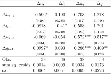
Table 1: Endogenous VAR: Austria

∆n

∆l

∆w

∆q

∆n

0.596* 0.190 -0.703 -1.278

(0.294) (0.235) (0.462) (1.048)

∆l

-0.0818 0.41* 0.553 1.291

(0.312) (0.249) (0.489) (1.110)

∆w

-0.069 -0.054 0.572*** 0.517**

(0.061) (0.048) (0.095) (0.215)

∆q

0.0997* 0.093 0.286*** 0.409**

(0.051) (0.040) (0.079) (0.179)

Obs. 38 38 38 38

sum sq. resids. 0.0014 0.0009 0.0034 0.0173 s.e. 0.0064 0.0051 0.0099 0.0226

*/**/*** denote significance at the 10%/5%/1% level Standard errors shown in parentheses

+ lowercase letters denote logarithmised variables, i.e.nt= ln(Nt)

For the Austrian VAR with completely endogenous variables we observe that for the labour demand equation lagged labour demand and lagged output enter positively and significantly. In the second equation, which describes labour supply, we only obtain a significant influence of the lagged dependent variable. The real wage equation shows that the real wage depends positively on its own lag as well as on past production changes. As for the output equation we observe that the one-period ahead real wage enters positively as well as past output.

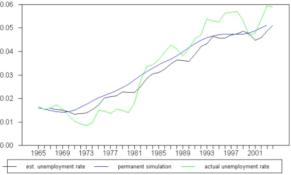
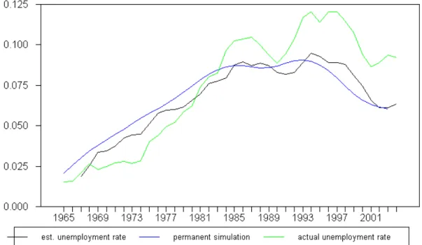
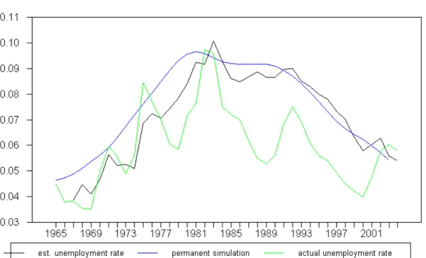
Figure 1 compares the actual unemployment rate with that predicted by the model.

We can see that the unemployment rate is overestimated until the early 1980s and underestimated from then onwards suggesting possibly a break around 1980.

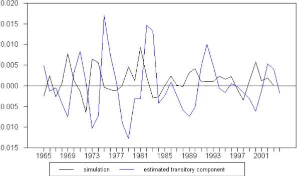
Comparing the transitory component that was computed subtracting the the HP-

filtered series from the actual series (estimated transitory component) with the one

implied by our model (simulation) in figure 2 it becomes apparent that the simulation

fluctuates less than the estimated and that the simulated precedes the estimated by

about one period.

Figure 1: Simulated vs. estimated unemployment rate

Figure 2: Transitory Component vs. Simulation

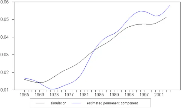
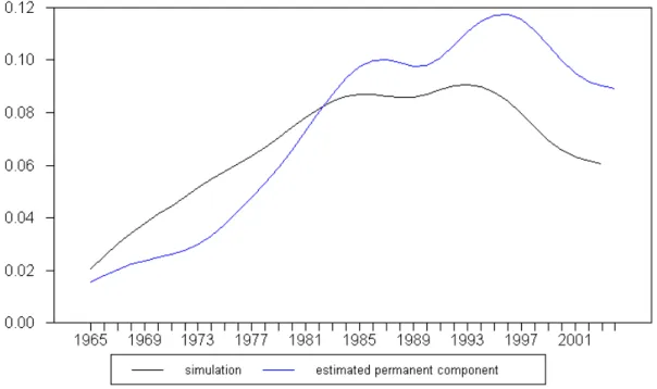
Figure 3: Permanent Component vs. Simulation

Comparing the smoothed series (estimated permanent component) with the simu- lated (i.e. implied by our estimated system) in figure 3 we observe the same pattern as in figure 1.

Therefore we would conclude that the permanent component has far greater ex- planatory power than the transitory component which was tested for by regressing the actual unemployment rate on the simulated transitory component on one hand and on the permanent component on the other hand. The results are displayed in table 2.

Table 2: Estimation Results and Explanatory Power of the Components dependent variable: ur

const. -0.013*** 0.031***

ur

0.449***

ur

-1.259

R

0.88 0.01

As can be observed from the table the transitory component has hardly any effect

on the unemployment rate as the R

is about 0.01.

3.1.2 France

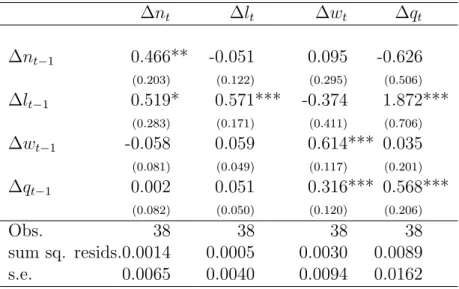
The results for the VAR with completely endogenous variables are displayed in table 3. For the labour demand equation only lagged employment and the labour force enter significantly. For labour supply only the lagged dependent variable exerts a significant and positive influence on the labour force.

As in the case of Austria real wage depends positively on its own lag and on lag output. Output depends on the labour force and on its own lag.

Table 3: Endogenous VAR: France

∆n

∆l

∆w

∆q

∆n

0.466** -0.051 0.095 -0.626

(0.203) (0.122) (0.295) (0.506)

∆l

0.519* 0.571*** -0.374 1.872***

(0.283) (0.171) (0.411) (0.706)

∆w

-0.058 0.059 0.614*** 0.035

(0.081) (0.049) (0.117) (0.201)

∆q

0.002 0.051 0.316*** 0.568***

(0.082) (0.050) (0.120) (0.206)

Obs. 38 38 38 38

sum sq. resids.0.0014 0.0005 0.0030 0.0089

s.e. 0.0065 0.0040 0.0094 0.0162

*/**/*** denote significance at the 10%/5%/1% level Standard errors shown in parentheses

Figure 4 compares the estimated and the actual unemployment rate for France.

Prior to 1980 the unemployment rate is overestimated by the model, from then onwards the reverse can be observed. After 1993 the gap between estimation and observed unemployment widens in addition.

From figure 5 which compares the estimated transitory component with the simu- lated (by the VAR system) transitory component it can be seen that fluctuations of both series are roughly equal in magnitude. Like in the Austrian case the simulation appears to precede the estimated transitory component.

Figure 6 compares the estimated with the simulated permanent component. The

relationship between the two appears to be similar to the one between the estimated

and the actual unemployment rate, which indicates that the explanatory power of the

permanent component might be more influential than the one of the transitory compo-

nent.

Figure 4: Simulated vs. estimated unemployment rate

Figure 5: Transitory Component vs. Simulation

Figure 6: Permanent Component vs. Simulation

Testing whether the transitory and permanent components exert a significant influ- ence on the development of unemployment, table 4 confirms the suspicion.

Table 4: Estimation Results and Explanatory Power of the Components dependent variable: ur

const. -0.021** 0.073***

ur

1.365***

ur

-0.830

R

0.88 0.01

3.1.3 UK

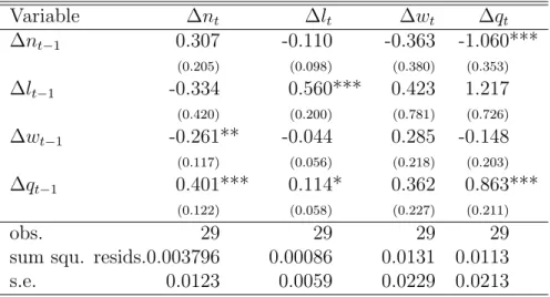
Table 5 presents the endogenous-VAR UK model.

The labour demand equation (∆n

) shows that the lagged real wage growth affects labour demand in the subsequent period negatively and significantly. On the other hand past growth of the economy in the year before will stimulate growth of the labour demand in the following year significantly.

As far as labour supply is concerned we obtained a positive effect of past growth of labour supply as well as a positive and significant effect of past production growth. As for output growth (∆q

) we see a negative and significant influence of labour demand one period ahead. On the other hand output growth is influenced by its own value one period ahead in a positive manner.

Table 5: Endogenous VAR: UK

Variable ∆n

∆l

∆w

∆q

∆n

0.307 -0.110 -0.363 -1.060***

(0.205) (0.098) (0.380) (0.353)

∆l

-0.334 0.560*** 0.423 1.217

(0.420) (0.200) (0.781) (0.726)

∆w

-0.261** -0.044 0.285 -0.148

(0.117) (0.056) (0.218) (0.203)

∆q

0.401*** 0.114* 0.362 0.863***

(0.122) (0.058) (0.227) (0.211)

obs. 29 29 29 29

sum squ. resids.0.003796 0.00086 0.0131 0.0113

s.e. 0.0123 0.0059 0.0229 0.0213

*/**/*** denote significance at the 10%/5%/1% level Standard errors shown in parentheses

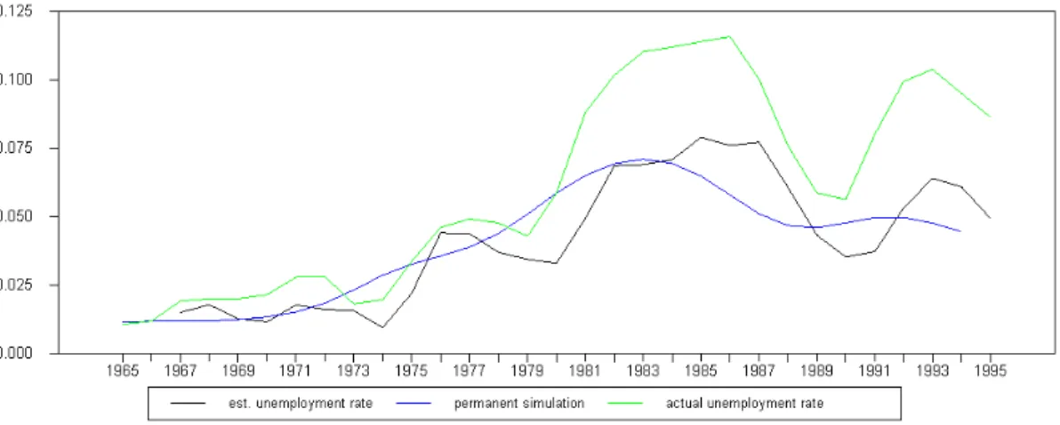
Figure 7 compares the actual unemployment rate with that implied by our model.

Even though the estimation-based forecast seems to do fairly well until the early 1980s, the gap between the estimated and the actual unemployment rate widens over the subsequent years with the exception of the reduction of unemployment between 1987 and 1990.

As figures 8 and 9 suggest this widening of estimation and actual unemployment rate can be largely attributed to the development of the permanent component simulation, which, with a minor exception in the mid-1970s, is always above the smoothed (i.e.

estimated) permanent component schedule. On the other hand the estimated and

simulated transitory components are close, even when the oscillations increase in the

1980s.

Figure 7: Simulated vs. estimated unemployment rate

Figure 8: Transitory Component vs. Simulation

Figure 9: Permanent Component vs. Simulation

Table 6 compares the explanatory power of both, transitory and the permanent component. For the UK case there is not much of a difference to the Austrian and French cases. The explanatory power of the permanent component is very high, whereas the explanatory power of the transitory component is virtually non-existent.

Table 6: Estimation Results and Explanatory Power of the Components dependent variable:ur

Constant -0.006 0.059***

ur

1.632***

ur

0.419

R

0.79 0.01 3.1.4 USA

For the US model with endogenous variables we find that most variables enter in a significant way. For the employment equation (∆n

) we observe that past production and past labour supply enter positively and significantly. The estimated effects are considerably stronger than in the respective equations of the other economies. In the labour supply equation all variables enter significantly (at least at a 10% level). Past production exerts a positive influence on labour supply as well as labour supply lagged one period. Past labour demand and past real wages display a negative influence on labour supply. For the real wage equation it can be observed that past labour demand negatively influences the real wage, whereas there is a significant and positive influence by labour supply as well as past production on the real wage. Labour demand affects output growth negatively and labour supply growth positively.

Similar to the other estimation results so far we see that until the early 1980s the estimated unemployment rates remains close to the actual unemployment rate, but for the remainder of the observation period our model overestimates actual unemployment (compare figure 10).

This result might be driven by the fact that the simulated permanent component of the unemployment rate is always larger than the estimated (in this case data generated).

For the transitory component of unemployment in the US the simulation oscillates less than the estimated transitory component.

Table 8 compares the explanatory power of the two unemployment components

for the US model. In contrast to all the previous models we observe a significant

contribution of the transitory component to unemployment, the explanatory power of

which amounts to about 8%. On the other hand the explanatory power of the permanent

component amounts to only 52%.

Table 7: Endogenous VAR: USA

∆n

∆l

∆w

∆q

∆n

-0.825*** -0.492*** -1.120***-2.148***

(0.284) (0.128) (0.295) (0.619)

∆l

0.757*** 1.026*** 0.791*** 1.927***

(0.205) (0.093) (0.213) (0.448)

∆w

-0.158 -0.147* 0.108 -0.217

(0.185) (0.083) (0.192) (0.403)

∆q

0.614*** 0.293*** 0.447** 1.093***

(0.142) (0.064) (0.148) (0.310)

obs. 38 38 38 38

sum squ. resids. 0.004 0.001 0.004 0.019

s.e. 0.011 0.005 0.011 0.023

*/**/*** denote significance at the 10%/5%/1% level Standard errors shown in parentheses

Figure 10: Simulated vs. estimated unemployment rate

Figure 11: Transitory Component vs. Simulation

Figure 12: Permanent Component vs. Simulation

Table 8: Estimation Results and Explanatory Power of the Components dependent variable: ur

const. -0.004 0.070***

ur

0.884***

ur

-1.164*

R

0.52 0.08

3.2 Exogenous VAR

In this section the unrestricted model was estimated for the same economies and the resulting models are now presented and discussed relative to the previous section.

3.2.1 Austria

In contrast to the endogenous model for Austria we observe that in the unrestricted VAR some variables which are not significant any more. As a result the fit of the single equations is not improved. Only for the real wage equation we observe an improved fit, where the standard error of the regression decreases from about 0.0099 to 0.0097.

For the real wage equation we see that there is a slightly significant influence of the past oil price on future payroll growth, but on the other hand past output does not exert influence on real wage growth any more.

As regards the explanatory power of the components it can be seen that this remains

unchanged.

Table 9: Exogenous VAR: Austria

∆n

∆l

∆w

∆q

∆n

0.548 0.380 -0.448 -1.072

(0.407) (0.325) (0.600) (1.4476)

∆l

-0.038 0.200 0.141 0.934

(0.447) (0.3576) (0.660) (1.591)

∆w

-0.087 -0.110 0.359** 0.493

(0.097) ( 0.078) (0.143) (0.345)

∆q

0.097 0.0627 0.211 0.395

(0.064) (0.0508) (0.094) (0.226)

∆ ln(ssc

) 0.0244 0.0386 0.137 -0.025

(0.043) (0.0347) (0.064) (0.1544)

∆ ln(p

) -0.0002 -0.003 0.001** 0.015

(0.004) (0.0029) (0.005) (0.0127)

r

-0.0005 -0.0001 -0.001 0.001

(0.0004) (0.0003) (0.001) (0.001)

Obs. 37 37 37 37

sum sq. resids. 0.0013 0.0008 0.0028 0.0163 s.e. 0.0065 0.0052 0.0097 0.0233

*/**/*** denote significance at the 10%/5%/1% level Standard errors shown in parentheses

Table 10: Estimation Results and Explanatory Power of the Components dependent variable: ur

const. 0.013*** 0.031***

ur

1.449***

ur

-1.259

R

0.88 0.01

Figure 13: Permanent Component vs. Simulation

Figure 14: Transitory Component vs. Simulation

Figure 15: Simulated vs. estimated unemployment rate

3.2.2 France

The French model with exogenous regressors better captures the effects in the labour supply and real wage rate equations, where the standard error of the regression is reduced.

For the labour demand equation we observe that the variance on the estimated coefficients gets larger. Also the magnitude of effects changes.

The real wage equations and the effects it displays is changed a lot due to the inclusions of exogenous regressors. On the one hand the lagged effect of real wage is reduced from about 0.61 to about 0.38, on the other hand we see that social security contributions display a positive and significant influence on real wage growth.

For the output equation we observe that the effect of past labour supply growth is slightly reduced whereas all other remain unchanged. No exogenous variable enters the equation significantly.

Table 11: Exogenous VAR: France

∆n

∆l

∆w

∆q

∆n

0.404* 0.095 0.030 -0.658

(0.234) (0.135) (0.294) (0.593)

∆l

0.730* 0.285 -0.371 1.987**

(0.368) (0.212) (0.462) (0.933)

∆w

-0.012 0.052 0.386*** 0.192

(0.115) (0.066) (0.144) (0.292)

∆q

0.023 0.019 0.320*** 0.577**

(0.088) (0.051) (0.110) (0.223)

∆ ln(ssc

) -0.026 0.021 0.065* -0.056

(0.030) (0.017) (0.037) (0.075)

∆p

-0.002 -0.002 0.008 0.000

(0.004) (0.002) (0.005) (0.010)

r

0.000 0.000 -0.001 0.000

(0.000) (0.000) (0.000) (0.001)

obs. 37 37 37 37

sum squ. resids. 0.001 0.004 0.002 0.009

s.e. 0.007 0.000 0.008 0.017

*/**/*** denote significance at the 10%/5%/1% level Standard errors shown in parentheses

As can be observed in table 12 the explanatory power of the transitory component

remains very small.

Figure 16: Simulated vs. estimated unemployment rate

Figure 17: Transitory Component vs. Simulation

Figure 18: Permanent Component vs. Simulation

Table 12: Estimation Results and Explanatory Power of the Components dependent variable: ur

const. -0.021** 0.072***

ur

1.3659***

ur

-0.829

R

0.88 0.01

3.2.3 UK

Table 13: Exogenous VAR: UK

∆n

∆l

∆w

∆q

∆n

0.304 -0.114 -0.294 -0.951***

(0.211) (0.100) (0.380) (0.332)

∆l

-0.331 0.562*** 0.378 1.146*

(0.430) (0.204) (0.774) (0.675)

∆w

-0.267** -0.050 0.407* 0.044

(0.132) (0.063) (0.237) (0.207)

∆q

0.401*** 0.114* 0.360 0.859***

(0.125) (0.059) (0.225) (0.196)

∆ ln(p

) 0.001 0.001 -0.018 -0.029**

(0.008) (0.004) (0.015) (0.013)

obs. 29 29 29 29

sum squ. resids.0.0038 0.00086 0.0123 0.0094

s.e. 0.00599 0.0227 0.01977

*/**/*** denote significance at the 10%/5%/1% level Standard errors shown in parentheses

Figure 19: Simulated vs. estimated unemployment rate

Figure 20: Transitory Component vs. Simulation

Figure 21: Permanent Component vs. Simulation

Table 14: Estimation Results and Explanatory Power of the Components dependent variable:ur

Constant -0.006 0.059***

ur

1.632***

ur

0.419

R

0.79 0.01

3.2.4 USA

Table 15 displays the US model with exogenous regressors. It can be seen that the inclusion of exogenous regressors improves the fit of almost all equations.

For the labour demand equation we observe that in contrast to the endogenous regressor model neither past labour supply nor lagged labour demand influence labour demand significantly. Instead, growth in social security contributions influences growth in labour demand positively and highly significantly.

For labour supply, our second equation in the system, we observe that all the effects that were significant in the endogenous-regressor model are now reduced in magnitude.

Real wage growth now does not influence labour supply growth any more. Again this effect might possibly be captured by the inclusion of social security contribution growth, which enters positively and significantly.

For the real wage equation past labour demand and past production exert a sig- nificant influence. But again, as in the previous models, the effects are reduced in magnitude.

The biggest change in the US model occurred in the output equation, where now only social security contribution growth enters the relationship significantly. All other variables, three of which had been highly significant before, are now insignificant. For the oil price effect it can be said that it is almost significant at the 10% level, which might be very intuitive as an explanatory factor for output growth.

Figure 22: Simulated vs. estimated unemployment rate

Table 15: Exogenous VAR: USA

∆n

∆l

∆w

∆q

∆n

-0.407 -0.396*** -0.926***-0.939

(0.290) (0.149) (0.354) (0.630)

∆l

-0.114 0.805*** 0.480 -0.170

(0.322) (0.165) (0.394) (0.701)

∆w

-0.063 -0.129 0.146 0.047

(0.163) (0.084) (0.200) (0.355)

∆q

0.399*** 0.242*** 0.360** 0.496

(0.146) (0.075) (0.179) (0.318)

∆ ln(ssc

) 0.177*** 0.047** 0.057 0.357***

(0.045) (0.023) (0.055) (0.099)

∆ ln(p

) -0.003 0.001 -0.008 -0.017

(0.005) (0.002) (0.006) (0.011)

r

0.000 0.000 0.000 0.001

(0.000) (0.000) (0.001) (0.001)

obs. 37 37 37 37

sum squ. resids. 0.003 0.001 0.004 0.012

s.e. 0.009 0.005 0.011 0.020

*/**/*** denote significance at the 10%/5%/1% level Standard errors shown in parentheses

Figure 23: Transitory Component vs. Simulation

Figure 24: Permanent Component vs. Simulation

Again, as in the endogenous regressor model, the US model with exogenous regres- sors is the only one where the transitory component has some explanatory power for unemployment.

Table 16: Estimation Results and Explanatory Power of the Components dependent variable: ur

const. -0.003 0.070***

ur

0.884***

ur

-1.164*

R

0.53 0.08

3.2.5 The Role of smoothing parameters for the explanatory power of the Permanent Component

Given the almost non-existent explanatory power of the transitory component in Aus- tria, France and the UK, this section will briefly examine the question whether the smoothing procedure or parameter is a key to understand these results.

For this purpose we used different smoothing parameters within the HP-framework to assess whether the explanatory power is dependent on the choice of the value of the smoothing parameter.

Figure 25 displays the relationship between the value of the smoothing parameter (λ

) and the explanatory power of both, the transitory and the permanent component for Austria, France and the US. Candidate Values for λ

are in the range between 7 and 100. The original suggestion of the literature for annual data was to use a power rule of two, which implies λ

= 100 for annual data. Ravn and Uhlig (2002), however, argued that a power rule of four might be more appropriate, which implies an approximate λ

of 7, which gives us the two points that define the interval.

As can be seen in figure 25 the choice of different power rules is influential in the European as well as US cases. Starting at the lower end and using λ

= 7 yields an R

of 0.88 in the European and 0.53 for the permanent component of unemployment in the US case. As we increase the value of the smoothing parameters the explanatory power of the permanent component also increases (0.9 for Austria and France and 0.57 for the US) At the same time the explanatory power of the transitory components vanishes entirely for the European cases as well as for the US case.

Therefore the explanatory power of the individual components is not invariant with

respect to the choice of the smoothing parameter.

Figure 25: Relation between smoothing parameters and explanatory power of all com-

ponents

Summary

In this study we estimated several vector-autoregressions and derived transitory and permanent components of unemployment rate, which was intended to closer investigate the chain-reaction theory of unemployment.

The empirical analysis points to the fact that the dynamics of labour force, em- ployment, wages and output do show significant differences among the countries under investigation. We have separated the key variables into permanent and transitory com- ponents and have tried to quantify the relative importance of the components for the evolution of unemployment

The estimation and simulation results suggest that the role of the transitory com- ponent of unemployment is minor in the case of Austria, France and the UK. Only a very small fraction of the development of unemployment can be explained by the transitory component. For the US-economy we find that around 8% of unemployment can be explained by the transitory component of unemployment. In all economies the permanent component of unemployment appears to be important.

The results support the view, that it is essential to analyse the dynamic adjustment processes at the labour market in order to understand the development of unemploy- ment. For economic policy it follows that measures have to take into account country specific adjustment processes. Furthermore the results point to the importance of a dif- ferentiated approach with respect to permanent and transitory labour market shocks.

Bibliography

Blanchard, Olivier, and Lawrence Summers (1986), “Hysteresis and the European Unemployment Problem,” NBER Macroeconomics Annual, vol. 1, Cambridge, Mass: MIT Press, 15-77.

Henry, Brian, Marika Karanassou, and Dennis J. Snower (2000), Adjustment Dynam- ics and the Natural Rate, Oxford Economic Papers, 52, 178-203.

Karanassou, M., Sala, H. and Snower, D. (2003): Unemployment in the European Union: a dynamic reappraisal, Economic Modelling, 20, 237-273.

Karanassou, Marika, and Dennis J. Snower (1997), Is the Natural Rate a Reference Point? European Economic Review, 41, 559-569.

Layard, Richard, Stephen Nickell, and Richard Jackman (1991), Unemployment, Ox-

ford: Oxford University Press.

Pesaran, M. Hashem, Yongcheol Shin, and Richard Smith (1996), “Testing for the Ex- istence of a Long-Run Relationship,” Working Paper No. 9645, CREST, Institut National de la Statistique et des Etudes Economiques.

Pesaran, M. Hashem (1997), “The Role of Economic Theory in Modelling the Long Run,” Economic Journal , 107(440), Jan., 178-191.

Phelps, Edmund S. (1994), Structural Slumps: The Modern Equilibrium Theory of Unemployment, Interest and Assets, Cambridge, Mass: Harvard University Press.

Ravn, M. O. and Uhlig, H. (2002): On Adjusting the Hodrick-Prescott Filter for the Frequency of Observations, Review of Economics and Statistics, vol. 84, no. 2, May 2002, pp. 371-76.

Sargent, Thomas J. (1987), Macroeconomic Theory, London: Academic Press.

Authors: Helmut Hofer, Robert M. Kunst, Wolfgang Schwarzbauer, Ulrich Schuh, Dennis J. Snower Title: Some Evidence on the Relevance of the Chain-reaction Theory in Selected Countries Reihe Ökonomie / Economics Series 207

Editor: Robert M. Kunst (Econometrics)

Associate Editors: Walter Fisher (Macroeconomics), Klaus Ritzberger (Microeconomics)

ISSN: 1605-7996

© 2007 by the Department of Economics and Finance, Institute for Advanced Studies (IHS),

Stumpergasse 56, A-1060 Vienna • +43 1 59991-0 • Fax +43 1 59991-555 • http://www.ihs.ac.at