Hydration and Ion Binding of Small Biologically Active Molecules: The Case
of Neurotransmitters
Dissertation zur Erlangung des Doktorgrades der Naturwissenschaften
(Dr. rer. nat.) der Fakultät für Chemie und Pharmazie der Universität Regensburg
vorgelegt von Sergej Friesen aus Ermak (KAZ)
2019
Promotionsgesuch eingereicht am: 14.10.2019 Tag des Kolloquims: 05.12.2019
Die Arbeit wurde angeleitet von: Apl. Prof. Dr. Richard Buchner Prüfungsausschuss: Apl. Prof. Dr. Richard Buchner
Prof. Dr. Dominik Horinek Prof. Dr. Joachim Wegener
Prof. Dr. Oliver Tepner (Vorsitzender)
meinen Eltern
Sophia und
Vorwort
Diese Arbeit entstand im Zeitraum vom Oktober 2017 bis Oktober 2019 am Institut für Physikalische und Theoretische Chemie der naturwissenschaftlichen Fakultät IV Chemie und Pharmazie der Universität Regensburg.
Allen voran möchte ich mich beim Herrn Apl. Prof. Dr. Richard Buchner für die Erteilung des Themas bedanken. Stete Unterstützung, diverse fachliche Diskussionen und seine wertvollen Ratschläge haben maÿgeblich zum Gelingen der Arbeit beigetragen. Auÿer- dem möchte ich ihm für das Ermöglichen von mehreren Konferenzteilnahmen und dem Forschungsauftenthalt danken.
Zudem möchte ich dem Leiter des Lehrstuhls, Herrn Prof. Dr. W. Kunz für die groÿzügige Unterstützung danken.
Ferner geht mein Dank and die zahlreichen Kooperationspartner:
•Herrn Prof. Dr. Glenn Hefter, Murdoch University, Western Australia, für die groÿzügige Unterstützung und zahlreichen fachlichen Diskussionen bei seinen alljährlichen Besuchen in Regensburg. Vor allem hinsichtlich der anorganischen Salzlösungen haben seinen Ratschläge wesentlich zu meinem Verständnis auf diesem Gebiet beigetragen und die Entstehung des Kapitel 4.1 wäre ohne ihn nicht möglich gewesen.
• Frau Prof. Dr. Marija Be²ter-Roga£, University of Ljubljana, Ljubljana, Slowenien, für das Bereitstellen der Leitfähigkeitsdaten von verdünnten Acetylcholinchlorid und Carba- chol Lösungen. Auÿerdem möchte ich mich für den zwar kurzen aber sehr interessanten Aufenthalt an ihrem Lehrstuhl bedanken.
• Frau Prof. Dr. Marina V. Fedotoca, Russian Academy of Sciences, G.A. Krestov In- stitute of Solution Chemistry, Ivanovo, Russland, für die fruchtbare Zusammenarbeit und die RISM Kalkulationen. Zudem möchte ich sie für die wertvollen Diskussionen auf den zahlreichen Konferenzen danken.
•Dem Verband der Chemischem Industrie e.V., Stiftung Stipendien-Fonds, für die Gewährung eines Doktorandenstipendiums.
Ohne diese Kooperationen und Zuwendungen wären groÿe Teile dieser Arbeit niemals möglich gewesen.
Vorwort
Allen Mitarbeitern und Kollegen des Lehrstuhls danke ich für die freundschaftliche Atmo- sphäre und Hilfsbereitschaft. Dabei richtet sich mein besonderer Dank an die (ehemaligen) Mitarbeiter des AK Buchner, M. Sc. Andreas Nazet und Dr. Nicolas Moreno, für die fre- undschaftliche Aufnahme in die Arbeitsgruppe, die Einweisung in die Messinstrumente und ihre zahlreichen Tipps, welche entscheidend zum Gelingen dieser Arbeit beigetragen haben. Ein ganz besonderer Dank geht an M. Sc. Andreas Nazet für die langjährige Zusammenarbeit und die Einführung in die Welt der dielektrischen Spektroskopie. Die fre- undschaftliche Arbeitsatmosphäre und seine stete Diskussionsbereitschaft über fachliche (oder auch nicht-fachliche) Themen waren für mich eine groÿe Bereicherung.
Ebenso bedanke ich mich ganz herzlich bei den internationalen Gästen Dr. Iwona Pªowa±- Korus, Dr. Vera Agieienko, Dr. Keiichi Yanase und Dr. Ziga Medo², mit denen ich in der Zeit der Entstehung dieser Arbeit zusammen arbeiten durfte.
Ganz besonders möchte ich auch meiner Familie und meiner Freundin Sophia danken, die mich jederzeit unterstützt haben.
Für die mentale Unterstützung am Arbeitsplatz möchte ich mich herzlich bei allen Teil- nehmern der Kaeerunde bedanken, welche für einen angenehmen Ausgleich gesorgt haben und deren tägliche Diskussionen mich zweifelsohne in meinem Leben bereichert haben.
Zu guter Letzt möchte ich allen Mitarbeitern der Werkstätten der Universität Regensburg für die schnelle und gewissenhafte Erledigung der Aufträge bedanken.
Contents
Motivation 1
1 Theory 5
1.1 Interaction of Electromagnetic Fields with Dielectric Materials . . . 5
1.1.1 Dielectric Polarization in Static Electric Fields . . . 5
1.1.2 Dielectric Properties in Alternating Electric Fields . . . 7
1.1.3 Response Function of Orientational Polarization . . . 9
1.2 Empirical Relaxation Models . . . 12
1.2.1 The Debye Equation . . . 13
1.2.2 Extensions of the Debye Equation . . . 14
1.3 Microscopic Relaxation Models . . . 15
1.3.1 The Onsager Equation . . . 15
1.3.2 The Kirkwood-Fröhlich Equation . . . 16
1.3.3 The Cavell Equation . . . 16
1.3.4 Debye Model of Rotational Diusion . . . 18
1.3.5 Relaxation by Discrete Jumps - The Case of Water . . . 19
1.3.6 Microscopic and Microscopic Relaxation Time . . . 20
1.4 Temperature Dependence of Relaxation Times . . . 21
1.4.1 Arrhenius Equation . . . 21
1.4.2 Eyring Equation . . . 21
2 Experimental 23 2.1 Materials . . . 23
2.2 Sample Preparation and Handling . . . 24
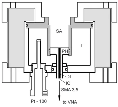
2.3 Measurement of Dielectric Properties . . . 25
2.3.1 Interferomentry . . . 25
2.3.2 Vector Network Analysis . . . 29
2.3.3 Processing of Experimental Data . . . 34
2.4 Supplementary Measurements . . . 35
2.4.1 Density . . . 35
2.4.2 Viscosity . . . 36
2.4.3 Electrical Conductivity . . . 36
2.5 Quantum Mechanical Calculations . . . 37 i
ii CONTENTS
2.6 Statistical Mechanical Calculations . . . 37
3 Neurotransmitters and Chemically Related Substances 39 3.1 Acetylcholine Chloride and Carbamylcholine Chloride . . . 40
3.1.1 Introduction . . . 40
3.1.2 Data Acquisition and Processing . . . 41
3.1.3 Choice of Relaxation Model and Assignment of Modes . . . 43
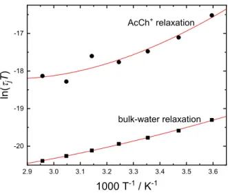
3.1.4 Activation Parameters of AcChCl(aq) Relaxation Processes . . . 47
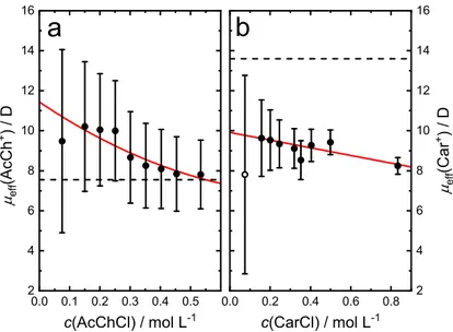
3.1.5 Solute Relaxations . . . 50
3.1.6 Solvent Relaxations - Hydration of AcChCl and CarCl . . . 55
3.1.7 RISM Calculations of AcChCl(aq) solutions . . . 61
3.1.8 Concluding Remarks . . . 64
3.2 Sodium Glutamate and Glutamine . . . 67
3.2.1 Introduction . . . 67
3.2.2 Data Acquisition and Processing . . . 68
3.2.3 Relaxation Models and Assignment of Modes . . . 69
3.2.4 Solvent Relaxations - Hydration . . . 75
3.2.5 Solute Relaxations . . . 82
3.2.6 Concluding Remarks . . . 84
3.3 γ-Aminobutyric Acid, α-Aminobutyric Acid &n-Butylammonium Chloride 87 3.3.1 Introduction . . . 87
3.3.2 Data Acquisition and Processing . . . 88
3.3.3 Choice of Relaxation Model and Assignment of Modes . . . 89
3.3.4 Solute Relaxations . . . 95
3.3.5 Solvent Relaxations - Hydration of GABA, AABA and BACl . . . . 101
3.3.6 Concluding Remarks . . . 107
4 Inorganic Salt Solutions 111 4.1 Magnesium Chloride and Calcium Chloride . . . 111
4.1.1 Data Acquisition and Processing . . . 112
4.1.2 Fitting Models and Assignment of Modes . . . 113
4.1.3 Solute Relaxations- Ion Pairing . . . 117
4.1.4 Solvent Relaxations - Ion Hydration . . . 120
4.1.5 Concluding Remarks . . . 124
4.2 Tetramethylammonium Chloride . . . 126
4.2.1 Introduction . . . 126
4.2.2 Data Acquisition and Processing . . . 127
4.2.3 Fitting Models and Assignment of Modes . . . 127
4.2.4 Solute Relaxation - Ion Pairing . . . 128
4.2.5 Solvent Relaxations - Ion Hydration . . . 132
4.2.6 Conclusion . . . 133
CONTENTS iii
5 Ternary Systems - Eect of Salts on the Neurotransmitter Solutions 135
5.1 Introduction . . . 135
5.2 Acetylcholine Chloride(aq) with Inorganic Salts . . . 136
5.2.1 Data Acquisition and Processing . . . 136
5.2.2 Fitting of the Spectra and Relaxation Models . . . 136
5.2.3 Eects of the Background Electrolyte . . . 137
5.2.4 Concluding Remarks . . . 145
5.3 Sodium Glutamate(aq) with Inorganic Salts . . . 145
5.3.1 Data Acquisition and Processing . . . 145
5.3.2 Choice of Relaxation Model and Assignment of Modes . . . 146
5.3.3 Eects of the Background Electrolyte . . . 149
5.3.4 Concluding Remarks . . . 156
5.4 Glutamine(aq) with Inorganic Salts . . . 157
5.4.1 Data Acquisition and Processing . . . 157
5.4.2 Choice of Relaxation Model and Assignment of Modes . . . 157
5.4.3 Eects of the Background Electrolyte . . . 160
5.4.4 Concluding Remarks . . . 164
Summary and Conclusion 167 A Supplemantary Measurement & Dielectric Relaxation Data 173 A.1 Acetylcholine Chloride and Carbamylcholine Chloride . . . 173
A.2 Sodium Glutamate and Glutamine . . . 181
A.3 γ-Aminobutyric Acid, α-Aminobutyric acid & n-Butylammonium chloride . 192 A.4 Electrolyte Solutions . . . 200
A.5 Ternary Systems - Eect of Salts on the Neurotransmitter Solutions . . . . 207
B Kinetic Dipolarization 237
C Correction of Raw Spectra for the Presence of IPs 241
Constants, Symbols and Acronyms
Constants
Elementary charge e0 = 1.60217739·10−19C
Permittivity of free space ε0 = 8.854187816·10−12C2J−1m−1 Avogadro's constant NA = 6.0221367·1023mol−1
Speed of light c = 2.99792458·108m s−1 Boltzmann's constant kB = 1.380658·10−23J K−1 Gas constant R = 8.3144598J K−1mol−1 Permeability of free space µ0 = 4π·10−7J2s2C−2m−1 Planck's constant h = 6.6260755·10−34J s
Symbols
α polarizability (C m2V−1) E~ electrical eld strength(V m−1) D~ dielectric displacement (C m−2) H~ magnetic eld strength(A m−1) P~ polarization (C m−2) ~j electric current density (A m−2) ˆ
γ complex propagation coecient (m−1) kˆ complex wave number(m−1) λm medium wavelength (m) εˆ complex permittivity
ε0 real part of εˆ ε00 imaginary part ofεˆ
µ dipole moment (C m) ηˆ generalized complex permittivity αm absorption coecient (Np m−1) β phase constant (m−1)
ε limν→0(ε0) ε∞ limν→∞(ε0)
T temperature (K) τ relaxation time(s)
t time (s) κ electrical conductivity (S m−1)
ν frequency(Hz) ω angular frequency (s−1) ρ density(kg m−3) c molarity (mol dm−3)
m mass (kg) η dynamic viscosity(Pa s)
ϑ temperature (◦C) b molality (mol kg−1)
I ionic strength (mol L−1) Λ molar conductivity (S m2mol−1)
CONTENTS v
Acronyms
MW microwave IR infrared
DR(S) dielectric relaxation (spectroscopy) MD molecular dynamics TDR time domain reectometry IB irrational bonding
IFM interferometer VNA vector network analyzer
H2O water EP electrode polarization
D Debye CC Cole-Cole
CD Cole-Davidson HN Havriliak-Negami
UV ultraviolet DFT density functional theory
EJM extended jump model NMR nuclear magnetic resonance OKE optical Kerr eect spectroscopy PCM polarizable continuum model RISM reference interaction site model PDF pair distribution function SDF spatial distribution function DMA dimethylacetamide
FA formamide PC propylene carbonate
DFT density functional theory IC ion-cloud
IP ion pair HO Hubbard and Onsager
SKA Sega, Kantorovich and Arnold CIP contact ion pair
SIP solvent-shared ion pair 2SIP solvent-separated ion pair
Motivation
General Aspects
Water is ubiquitous. Water is the most common liquid on our planet and it is essential for life to exist. It constitutes ∼ 50−70 % of the cell content, where it does not simply act as a medium but rather plays a fundamental part in all biological processes. As pointed out by Ball in his famous review on water in biological systems, it is a substance that actively engages and interacts with biomolecules in complex, subtle, and essential ways [1]. For instance, folding, stabilization and dynamics of proteins and hence their activity are governed by their hydration [26]. Further, ligand recognition and the kinetics and thermodynamics of binding in biological processes are majorly controlled by the solvation of both, the ligand and the receptor [4, 79].
Despite the emergence of many dierent techniques to study the solvation of various so- lutes during the last decades, fundamental rules and guidelines for the description of the hydration structure and dynamics are still lacking. On the one hand, this might originate from the fact that dierent techniques probe dierent hydration characteristics and an unied denition of hydration water does not exist [10]. For example, nuclear magnetic resonance [11, 12], neutron scattering [1315] and statistical mechanical calculations [16 18] report only short-range eects at a timescale greater than the picosecond regime, while most MD simulations [19], terahertz [20, 21] and dielectric spectroscopy studies [22] inves- tigate the (collective) dynamics and structure of the solutions, including long-range eects, at shorter picosecond/sub-picosecond timescales. However, keeping in mind that each in- dividual technique examines dierent aspects of hydration by probing dierent solvation phenomena at dierent timescales, a coherent picture can sometimes still be deduced by combining the results of the individual techniques [10].
On the other hand, this lack of universal guidelines might just reect the whole complexity of solvation and the inability of combining all the specic hydration phenomena of dierent classes of solutes (charged/uncharged, hydrophilic/hydrophobobic, macromolecules/small molecules) into one unied concept.
The situation is fairly odd for the hydration of larger biomolecules, e.g. proteins. In spite of many investigations of these systems (see Refs. [23], [10] and [1] for an overview), basic principles for understanding the solvation of these macromolecules have not really been established yet. Probably the main reason for this is that comparably few work has been done on small, biologically relevant molecules, which could serve as simplied model
1
2 Motivation
species, and thus it may not be possible either to generalize or to reduce the structural and dynamic aspects of hydration to simplistic rules of thumb [1]. Amino acid solutions would certainly be appropriate candidates for such studies.
The eect of ions on aqueous systems containing biomolecules is even more baing. Un- derstanding and interpreting specic ion eects has concerned physical chemist for over hundred years. Franz Hofmeister was the rst to study the eect of ions on the precipita- tion of egg white protein and he proposed a series for their respective eciency to do so [24, 25]. Today it is known that the empirical Hofmeister eect depends on many dierent aspects of the present solution, e.g. buer, pH or polarity of the protein surface, and the series may even be reversed if one of these factors is varied [26, 27]. These specic ion eects cannot be explained by conventional electrostatic theories (DLVO, Debye-Hückel, etc.). A subtle interplay between local, rather than long-range, ion-water-biomolecule in- teractions seems to govern the ability (or disability) of ions to bind to distinct moieties of the biomolecule [28].
About 20 years ago, Collins introduced a more sophisticated approach, which is often called the Collins's rule or law of matching water anities. In this concept, electrostatics and hydration eects of each individual ion are automatically taken into account. Many ion specic phenomena could successfully be explained by it [2931]. On the other hand, this concept merely considers ion-ion interactions, which renders impossible its application to explain specic interaction of ions with uncharged entities e.g. in biological systems [29].
All these concepts of ions often involve the terms structure-making and structure- breaking ions [32], or the more or less equivalent appellations kosmotrope or chaotrope [33], which try to classify ions according to their inuence on the H-bond network of water.
Loosely speaking, structure-makers (or kosmotropes) refer to highly-solvated ions of high surface charge density and structure-breakers (or chaotropes), on the other hand, designate weakly hydrated, rather large ions. However, a clear classication of ions into the corre- sponding categories often depends on the applied experiment. In addition to that, there seems to be no consensus of how to properly quantify a water-structure experimentally, which makes this classication even more puzzling [34].
It seems that despite recent advances in the eld of solute-solvent and specic ion interac- tions, many questions are still open and nding answers to at least some of these matters could be of crucial importance for chemistry, biochemistry and chemical engineering.
However, in order not to get hopelessly lost in its complexity, it is instructive to focus on a certain class of small (bio-)molecules. Thorough investigations of their physico-chemical behaviour in aqueous solution could infer information on the solute-solute and solvent- solvent interactions. These data, in the case of biologically relevant solutes, could shed some light on their biological activity and, on the other hand, could potentially be used for the construction of models for other solutes.
Neurotransmitters (NTs) belong to the class of small, biologically active molecules. Despite their great importance, detailed investigations of their solvation and dynamics in aqueous
Motivation 3
solution are rather scarce. Interestingly, most studies of these systems were highly focused on the NT-conformation [3540, 40, 41], often neglecting other signicant solvent-solute and solute-solute eects, which might be equally if not even more important for their bio- logical action.
Aim of this Study
The general aim of this thesis is the investigation of the structure and dynamics of aqueous solutions of neurotransmitters and other chemically-related, biologically relevant molecules by the means of dielectric relaxation spectroscopy (DRS) in the megahertz to gigahertz frequency range. The present study can be subdivided into three main parts:
In the rst part of the experimental results, a detailed study of the complex permit- tivity spectra of binary neurotransmitter solutions and chemically related compounds is described. Therefore, concentration-dependent measurements are performed at 25 °C to in- fer information on the hydration, dynamics and ion-binding properties of the biomolecules.
For the cationic NTs acetylcholine and carbomoylcholine additional insight into the dy- namical properties of the various relaxation processes will be gained by measuring the dielectric spectra over a wide range of temperatures. Further, the dielectric data of the latter systems will be accompanied by dilute-conductivity measurements and statistical mechanical calculations (1D-and 3D-RISM) to provide as detailed description as possible on the behaviour of these NTs in solution.
The proteinogenic amino-acid and neurotransmitter L-glutamate will be compared to the structurally-related amino-acid L-glutamine, while the investigation of the NT γ- aminobutyric acid and its isomerα-aminobutyric acid will reveal structural and dynamical information on the eect of changing position of the amine moiety at these biomolecules.
The second part deals with binary solutions of inorganic salts. The hydration and ion-pair formation in aqueous MgCl2, CaCl2 and Me4NCl solutions is studied. The Me4N+cation is of particular interest due to its special hydrophobic/hydrophobic balance and its structural relation to many biologically important compounds, while Mg2+ and Ca2+ are omnipresent in living organisms. Although these systems were extensively studied in previous works [14, 4249], precise and systematic dielectric relaxation studies over a wide frequency range were still lacking.
In the last portion of this thesis, eects of addition of inorganic, biologically-relevant salts to biomolecule solutions will be investigated. Ion-binding eects and the impact of salts on the acetylcholine, glutamate and glutamine hydration will be studied. Possible structures of ion aggregates and their degree of association will be deduced. By varying the cations or the anions, respectively, specic ion eects can also be studied in this way. These ternary solutions represent much better the real conditions in living systems, which involve a great number of various solvated ions interacting with the bioactive solute.
4 Motivation
A special focus of this thesis will be the interpretation of the DRS results on a microscopic level with the aid of quantum chemical calculation of various low-energy conformers of the investigated molecules. Comparisons of these results with other theoretical and experi- mental approaches will be drawn, with the aim to provide a coherent picture and thus to build a bridge between the dierent techniques.
To address all issues mentioned above, proper analysis of the DR spectra is prerequisite.
Thus, new mathematical approaches for the analysis of the relaxation parameters and for the correction of the DR spectra for interfering relaxation modes were developed and utilized in this work.
Chapter 1 Theory
1.1 Interaction of Electromagnetic Fields with Dielec- tric Materials
1.1.1 Dielectric Polarization in Static Electric Fields
When applying a static electric eld to dielectric matter, charge displacement occurs. The type of the displacement depends on kind of charges present in the system. In the case of free charges, e.g. (dilute) electrolyte solutions, a translational motion of positive and negative charges towards the respective electrodes can be observed. For bound pairs of positive and negative charge, i.e., dipoles, the applied eld induces a reorientation of the dipoles such that the dipole moment vectors align themselves parallel to the eld, min- imizing their potential energy. The two cases represent conduction through an electric current and conduction through a displacement current, respectively. Note that the latter is a transient process and occurs until the dipoles reach their new equilibrium orientation which is determined by the interplay between intermolecular interactions, the electric eld and thermal energy. A system comprising both kinds of charges, free charges and perma- nent or induced dipoles, is often referred as real dielectric [50], as it most appropriately describes the situation in many real systems, e.g. salt solutions, ionic liquids etc.
Mathematically, the response of a material to an applied low-intensity* electric eld, E~, is described by the phenomenon of polarization, P~. The polarization, which is dened as the macroscopic dipole moment of the system per unit volume, of an isotropic and uniform system is connected to the electric eld via
P~ = (ε−1)ε0E~ (1.1)
In Eq. 1.1,ε0 is the permittivity of free space andεthe relative permittivity of the sample.
The factor (ε−1) is also known as the electrical susceptibility.
*For eld strengths of∼106V/m or higher non-linear eects become noticeable. Within the scope of this thesis the non-linear eects are unimportant and thus no further description of these eects will be pursued. The subsequent derivation of the mathematical equations refers to the linear response only.
5
6 CHAPTER 1. THEORY
Following the approach of Maxwell, which treats matter as continuous charge distribution, the electric eld inside the material is the result of electric displacement, D~, which is connected to polarization by
D~ =ε0E~ +P~ =ε0ε ~E (1.2) To be able to extract information on molecular-level processes from polarization, it is convenient to split up P~ into two distinct contributions [51]:
P~ =P~µ+P~α (1.3)
where P~µ is the orientational (dipolar) polarization, which can be written as P~µ=X
k
ρkh~µki (1.4)
and P~α is the induced polarization, given by P~α =X
k
ρk~µk,ind=X
k
ρkαk(E~i)k (1.5) In Eqs. 1.4 and 1.5, ρk is the number density of particles k, h~µki is the ensemble average of the permanent dipole moment, which can be obtained from Langevin theory taking into account all particle orientations, and ~µk,ind is the induced dipole moment. The latter can be expressed by the molecular polarizability, αk, and the avarage local eld acting upon the particle,(E~i)k. This local eld does not coincide with the applied external eld nor the permanent dipole moment vector ~µ of the regarded species but it is a superposition of all sources of electric eld at the position of the particle k minus the eld due to the particle itself.
Orientational polarization, P~µ, is the result of partial alignment of a species with a perma- nent dipole moment against thermal motion in an applied electric eld. The intermolecular interactions and the inertia of the species lead to a nite time for the establishment of full polarization. For molecular liquids the characteristic time is at the pico- to nanosecond timescale, corresponding to frequencies in the microwave region.
The induced polarization,P~α, itself comprises two contributions, namely the atomic polar- ization, resulting from the relative shift of the core positions, and the electron polarization, due to the uctuations of the electron sheath density relative to the core. These two pro- cesses are rather fast and their characteristic frequency is located in the infrared and ultraviolet range, respectively.
SinceP~µandP~αoccur at signicantly dierent timescales, both eects can be well separated on the frequency scale and can be regarded as linearly independent. By the incorporation of the induced polarization contribution into the innite frequency permittivity, ε∞, one may write in the style of Eq. 1.1:
P~µ =ε0(ε−ε∞)E~ (1.6)
P~α =ε0(ε∞−1)E~ (1.7)
1.1. INTERACTION OF ELECTROMAGNETIC FIELDS WITH DIELECTRIC
MATERIALS 7
The value of innite frequency permittivity, ε∞, is usually determined in the far-infrared region, at around 200 cm−1, and it states the permittivity after the decay of the orienta- tional polarization [52]. In practice, the value extrapolated to higher frequencies from the measurements in the microwave frequency range is often taken for ε∞.
1.1.2 Dielectric Properties in Alternating Electric Fields
As can be seen above, time is an important variable when talking about polarization of material, as certain processes require characteristic periods of time to establish a certain value of polarization. Whereas the polarization is in equilibrium with the electric eld in the static case, it does not necessarily have to be for the time-dependent electric elds.
This so-called dynamic case can most easily be described with the help of a harmonic, e.g. sinusoidally, oscillating electric eld, E(t)~ˆ , with the amplitude, E~0, and the angular frequency, ω= 2πν:
~ˆ
E(t) =E~0exp (iωt) (1.8)
If the frequency of the electric eld is suciently low, the microscopic particles in the condensed matter will be able to follow the electric eld instantaneously (quasi-static case, see above). The frequency threshold until which the quasi-static conditions apply depends strongly on type of material and the temperature, and for liquids far from their glass- transition temperature it lies typically between 1 MHz and 1 GHz [53]. Exceeding this frequency, the microscopic particles cannot follow the changes in the electric eld anymore, which leads to a frequency-dependent phase delay δ(ω)between the harmonic electric eld and the dielectric displacement. Therefore one may write:
~ˆ
D(t) =D~0exp [i(ωt−δ(ω))] (1.9) where D~0 is the amplitude of the sinusoidal variation. Using the same relation between
~ˆ
E(t) and D(t)~ˆ as given in Eq. 1.2 for the static case, the complex, frequency dependent permittivity, ε(ω)ˆ , can be introduced:
ˆ ε(ω) =
D~0
ε0E~0 exp [−iδ(ω)] (1.10) By using the Euler's relation
ˆ
ε(ω) =ε0(ω)−iε00(ω) (1.11) is nally obtained, whereε0(ω) = D~0
ε0E~0cos[δ(ω)]andε00(ω) = D~0
ε0E~0sin[δ(ω)]. Both quantities are interconnected through the Kramers-Kronig relation and can be converted into each
Electric elds always give rise to magnetic elds and vice versa, thus the electromagnetic theory must be used. Mostly, however, it is sucient to consider the electric eld only. Theˆsymbol denotes that the quantity is expressed as a complex function.
8 CHAPTER 1. THEORY
other. For ω = 0 equation 1.10 reduces to the static-case relation 1.2 with ε0(ω) = ε, thereforeε0(ω)can be considered as a generalization of the dielectric constant for oscillating elds and describes the dispersive in-phase response. The dissipative out-of-phase response, ε00(ω), (with a phase shift of π/2 with respect to E(t)~ˆ ) determines the loss of energy in the dielectric. Consequently, ε00(ω) is called the dielectric loss.
The energy dissipated per unit of time in an ideally insulating dielectric is given by W˙ = 1
2ωE02εoε00(ω) (1.12)
However, in reality most dielectrics show a certain electrical dc conductivity contribution, κ. This leads to an electrical current density, ~jˆ, which is in phase with the electric eld and is given by
~j(t) =ˆ κE(t)~ˆ (1.13)
The dissipated amount of energy per unit of time by the electric current can be obtained from Joule's law
W˙ = 1
2κE02 (1.14)
From the comparison of equations 1.12 and 1.14, it becomes clear that the absorption of energy in a dielectric material is determined by the sum ε00(ω) +κ/(ε0ω). As long as κ is constant, no diculties in separation of the eects of conduction and polarization arise. However, when it takes a certain time for the current to reach its equilibrium value, equation 1.13 has to be replaced by
~j(t) = ˆˆ κ(ω)E(t)~ˆ (1.15) where
ˆ
κ(ω) =κ0(ω)−iκ00(ω) (1.16) analogous to the complex representation of ε(ω)ˆ . The quantity κ0 determines the part of the current which is in-phase with the applied eld and leads to the energy absorption, while the imaginary part,κ00, gives the part of current with a phase shift ofπ/2with respect to the eld. The combination of dielectric displacement and the electrical current in the form of a generalized dielectric displacement (for details see [51]) leads to the introduction of the experimentally accessible generalized complex permittivity, η(ω) =ˆ η0(ω)−iη00(ω), with its real part
η0(ω) =ε0(ω)− κ00(ω)
ωε0 (1.17)
and the imaginary part
η00(ω) =ε00(ω) + κ0(ω)
ωε0 (1.18)
An univocal separation of ε(ω)ˆ and κ(ω)ˆ is impossible, as long as the molecular origin of the various contributions to η(ω)ˆ is unknown. Generally, reorientations of dipoles or
1.1. INTERACTION OF ELECTROMAGNETIC FIELDS WITH DIELECTRIC
MATERIALS 9
charge displacements within particles must be attributed to the ε(ω)ˆ , while translational processes of charges are governed byκ(ω)ˆ . Some dispersion of the complex conductivity can be explained by the classical theory of Debye and Falkenhagen [54] for electrolyte solutions and is thought to be the result of ion-cloud relaxations. However, quantitative approaches for the separation of ε(ω)ˆ and κ(ω)ˆ are still lacking [55]. The inability of determining the two contributions independently particularly aects the analysis of dielectric properties of conductive systems. To circumvent this problem, the dc conductivity, κ = κ0(0) = ˆκ(0), can be used to account for the frequency-independent contribution of conductivity whereas potential frequency-dependent processes are covered byε(ω)ˆ . Thus, the complex dielectric permittivity can be calculated as
ε0(ω) =η0(ω) (1.19)
ε00(ω) =η00(ω)−κ0(0)
ωε0 (1.20)
Using this approach,ε0andε00can be obtained from the experimentally accessible quantities η0,η00andκ. Note that the second term on the right-hand side of Eq. 1.20 strongly increases at decreasing frequencies, thus it determines the minimum frequency down to which precise ˆ
ε(ω)spectra are available in the experiment [52].
1.1.3 Response Function of Orientational Polarization
As mentioned in Section 1.1.1, orientational polarization does not occur instantaneously but requires a certain time due to inertia and friction acting on the reorienting particles.
Thus, for suciently high frequencies of the electric eld the dipoles are not able to follow the eld variation and the polarization can not attain its maximum value anymore. In this case the response function gives the relation between E~ˆ and P~ˆ. To derive the response function for an isotropic and linear dielectric a thought experiment has to be considered.
The thought experiment is visualized in Figure 1.1. A static electric eld E(t) =~ E~0, causing the polarizationP~(t) = P~0, is switched o att= 0 and a decay of the polarization can be observed. While the induced polarization is assumed to drop instantaneously,P~µ(t) decreases monotonically with t.
In a linear dielectric the superposition principle applies e.g. for electric elds and the respective induced polarizations.
10 CHAPTER 1. THEORY
Figure 1.1: Evolution of (a) E(t)~ , being cut o at t= 0, and (a) the polarization, P~(t). The time evolution of the remaining orientational polarization can be expressed as [51]
~ˆ
Pµ(t) =P~ˆµ(0)·FPor(t) with FPor(0) = 1, FPor(∞) = 0 (1.21) where the step response function (time domain autocorrelation function) FPor(t)is dened as [52]
FPor(t) =
DP~ˆµ(0)·P~ˆµ(t)E
DP~ˆµ(0)·P~ˆµ(0)E (1.22) The step response function is directly accessible via time domain experiments, e.g. Time Domain Reectometry (TDR) [56, 57].
1.1. INTERACTION OF ELECTROMAGNETIC FIELDS WITH DIELECTRIC
MATERIALS 11
However, from an experimental point of view, frequency domain experiments are of a greater interest. A time-dependent electric eld can be approximated by splitting it up in an innite number of dierential square pulses. Thus, for a harmonically oscillating electrical eld the orientational polarization at any time t can be written as
~ˆ
Pµ(ω, t) = ε0(ε−ε∞)E(t)~ˆ Z ∞
0
exp(−iωt0)fPor(t0)dt0 (1.23)
where fPor(t0) is the pulse response function in the time domain and is the negative time- derivative of the normalized step response function:
fPor(t0) =−∂FPor(t−t0)
∂(t−t0) normalized according to Z ∞ 0
fPor(t0)dt0 = 1 (1.24)
The integral in Eq. 1.23 is the Laplace-transformed pulse response function of the orien- tational polarization:
Z ∞ 0
exp(−iωt0)fPor(t0)dt0 =Liω[fPor(t0)] (1.25)
By comparing equation 1.6, modied accordingly for oscillating elds, and Eq. 1.23 the connection between the complex permittivity and the Laplace-transformed pulse response function becomes evident [51]:
ˆ
ε(ω) =ε0(ω)−iε00(ω) =ε∞+ (ε−ε∞)· Liω[fPor(t0)] =ε∞+ (ε−ε∞)·F(ω) (1.26) Here, the pulse response function (often referred as relaxation or band-shape function), F(ω), is the representation of the autocorrelation functionFPor(t) in the frequency domain and comprises equivalent information on the relaxation dynamics [52].
As can be seen from the model broadband dielectric spectrum in Figure 1.2, relaxation bands are rather broad due to its coupling to the surrounding medium compared to the sharp absorption peaks of the intramolecular processes in the IR or UV range. The latter processes, which are covered by P~α, obey the rules of quantum mechanics and give rise to resonant vibrational transitions at infrared frequencies and resonant electronic transitions in the ultraviolet range, respectively [58].
12 CHAPTER 1. THEORY
'()
log( ) 1
P
''()
P
Dielectric Relaxation
Vibrational Transitions
Electronic
Transitions
MW IR UV
Figure 1.2: Schematic complex permittivity spectrum, with ε0(ν) (dashed line) and ε00(ν) (solid line), covering frequencies from the microwave (MW) regime to infrared (IR), and up to the ultraviolet (UV) region.
Since the present work does not treat intramolecular resonance processes, but focuses on the dielectric relaxation in the microwave frequency range, various mathematical descriptions of the dielectric relaxation functions will be presented in the following chapter.
1.2 Empirical Relaxation Models
Numerous empirical and semi-empirical approaches have been proposed in literature to characterize dielectric relaxation phenomena. In general, the dielectric spectra of liquids and solutions (far from their glass-transition temperature) can be decomposed into their individual contributions and described with a suitable linear combination of n single re- laxation processes:
ˆ
ε(ω) =ε∞+
n
X
j=1
(εj−ε∞,j)Fj(ω) (1.27) All single processes are assumed to be linearly independent and each process,j, is charac- terized by its own band-shape function, Fj(ω), and amplitude, Sj:
ε−ε∞=
n
X
j=1
(εj−ε∞,j) =
n
X
j=1
Sj with ε∞,j =εj+1 (1.28)
1.2. EMPIRICAL RELAXATION MODELS 13
Yet, it should be emphasized that many of the proposed models are (semi-) empirical and thereby their physical meaning is often not easy to derive. In the following, models used in this work will be presented.
1.2.1 The Debye Equation
The simplest approach to model dielectric relaxations was introduced by Debye [59], who assumed the decrease of the orientational polarization after the cut-o of the external electric eld to be directly proportional to the momentary polarization itself [60]. One thus obtains a dierential time law of rst order
∂
∂t
P~µ(t) = −1 τ
P~µ(t) (1.29)
where τ is the relaxation time of this process, characterizing the dynamics of the system.
Solving the dierential equations leads to
P~µ(t) =P~µ(0)exp
−t τ
(1.30) Comparing Eqs. 1.21 and 1.30 yields the step response function in the time domain
FPor(t) = exp
−t τ
(1.31) and after application of Eq. 1.24 the pulse response function of the Debye relaxation is obtained:
fPor(t) = 1 τexp
−t τ
(1.32) According to Eq. 1.26 the complex permittivity can be obtained by Laplace transformation of the pulse response function
ˆ
ε(ω) =ε∞+ (ε−ε∞)· Liω 1
τexp
−1 τ
(1.33) Using the identity Ls[exp(ax)] = (s−a)−1 [51] the complex permittivity can be written as the Debye (D) formula
ˆ
ε(ω) =ε∞+ ε−ε∞
1 +iωτ (1.34)
The comparison of the Eqs. 1.34 and 1.26 provides the relaxation function, FD(ω), of the Debye equation
FD(ω) = 1
1 +iωτ (1.35)
Eventually, the real and the imaginary parts of ε(ω)ˆ can easily be obtained from Eq. 1.34 ε0(ω) =ε∞+ ε−ε∞
1 +ω2τ2 (1.36)
ε00(ω) =ωτ ε−ε∞
1 +ω2τ2 (1.37)
14 CHAPTER 1. THEORY
The dispersion curve, plotted asε0 =ε0(ln(ω)), is a point symmetric, monotonically decreas- ing function with the inection point at ω = 1/τ. The absorption curve, ε00 = ε00(ln(ω)), yields an axis-symmetric band reaching its maximum at ω = 1/τ.
1.2.2 Extensions of the Debye Equation
For many condensed systems deviations from the mono-exponential relaxation described by the Debye band-shape function occur. In this case, the assumption of just one relaxation time is dropped and the analysis of these dielectric spectra is improved by the introduc- tion of the concept of a continuous relaxation time distribution function, g(τ), proposed by Wagner [61]. The logarithmic distribution function, G(ln(τ)), is often preferred for practical reasons. The complex permittivity can be written as
ˆ
ε(ω) = ε∞+ (ε−ε∞) Z ∞
0
G(ln(τ))
1 +iωτ dln(τ)with Z ∞ 0
G(ln(τ))dln(τ) = 1 (1.38) If G(ln(τ)) is a delta function, this equation will reduce to a Debye function.
In the literature a lot of aord has been made to obtain the distribution function directly from experimental results, which turned out to be anything but straightforward and a gen- erally accepted theory of the origin of the non-Debye behaviour is still lacking until today.
However, the introduction of additional parameters into the Debye equation 1.34 made it possible to describe the relaxation behavior satisfactorily. These empirical parameters lead to symmetrical and/or asymmetrical broadening of the dispersion curves, which can be interpreted as a respective broadening of the distribution of relaxation times around its most probable relaxation time value τ0 [51].
Cole-Cole equation
The Cole-Cole (CC) equation [62, 63] describes a symmetrical relaxation time distribution around a principal relaxation time τ0 by introducing the parameter α ∈ [0...1[ into the Debye equation
FCC(ω) = 1
1 + (iωτ0)1−α (1.39)
For α= 0 the CC equation reduces to the Debye equation. Increasing the α-value results in a systematical broadening of the dispersion and the dissipative curves.
Cole-Davidson equation
An asymmetrical relaxation time distribution around the center of gravity τ0 is given by the Cole-Davidson (CD) equation [64, 65]. The empirical parameter β ∈]0...1]introduces an asymmetric broadening of dispersion and absorption curves towards higher frequencies.
The CD equation is
FCD(ω) = 1
(1 +iωτ0)β (1.40)
1.3. MICROSCOPIC RELAXATION MODELS 15
and it reduces to the Debye equation for β = 1. Havriliak-Negami equation
Combining both parametersα∈[0...1[andβ ∈]0...1], leads to the Havriliak-Negami (HN) equation [66] for broad, asymmetric relaxation time distributions:
FHN(ω) = 1
(1 + (iωτ0)1−α)β (1.41) Consequently, the HN equation is used for the description of broad and asymmetric dis- persion and dissipative curves. For α = 0 and β = 1 the Debye band-shape function is obtained.
Furthermore, corrections for the unphysical behavior of the mentioned equations in higher frequency regions (THz and far-infrared regime) can be introduced. As the Debye, but es- pecially the broader CC, CD and HN equations, decay too slowly a termination at higher frequencies is necessary, which accounts for the inertia eects of the relaxing species. How- ever, as this correction was not needed for the present work, it is not going to be elucidated further. For more details see [67].
1.3 Microscopic Relaxation Models
So far dielectric relaxation has been discussed on a macroscopic level and the formal de- scription of the experimental data using the equations in the previous section only yields macroscopic parameters, such as amplitude, Sj, and relaxation time, τj. In order to es- tablish the link between the macroscopic and the microscopic properties some suitable theoretical models will be presented in the following.
1.3.1 The Onsager Equation
The Onsager model [51, 68] is based on the concept of a single dipole being placed into a cavity, which itself is embedded in an innite continuum characterized by its macroscopic properties. Assuming a spherical cavity and neglecting specic interactions as well as the anisotropy of the surrounding electric eld yields the equation
ε0(ε−1)E~ =E~h ·X
j
ρj 1−αjfj
αj + 1
3kBT · µ2j 1−αjfj
(1.42) where ρj is the dipol density, αj the polarizability, fj the reaction eld factor and µj the dipole moment of the speciesj.
For the case of spherical cavity, the cavity eld E~h can be expressed as E~h = 3ε
2ε+ 1
E~ (1.43)
16 CHAPTER 1. THEORY
with ε denoting the permittivity of the continuum dielectric.
Combining Eqs. 1.42 and 1.43 leads to the general form of the Onsager equation ε0(ε−1)(2ε+ 1)
3ε =X
j
ρj 1−αjfj
αj + 1
3kBT · µ2j 1−αjfj
(1.44) For a pure single-component dipole liquid with non-polarizable molecules, exhibiting just one dispersion step, this equation reduces to
(ε−ε∞)(2ε+ε∞)
ε(ε∞+ 2)2 = ρµ2
9ε0kBT (1.45)
Hence, the dipole moment of a species can be calculated from the above equation if the density, the static permittivity and ε∞ are known. However, the Onsager equation is only valid for systems without dipole-dipole correlations, which generally does not necessarily hold for liquids.
1.3.2 The Kirkwood-Fröhlich Equation
To account for the shortcoming of the lack of specic particle interactions Kirkwood and Fröhlich [69, 70] introduced, with the help of statistical mechanics, the correlation factor gK. The Kirkwood-Fröhlich equation reads
(ε−ε∞)(2ε+ε∞)
ε(ε∞+ 2)2 = ρµ2
9ε0kbT ·gK (1.46)
The correlation factor describes the orientation correlation between the dipole and the neighbor molecules. Taking only nearest-neighbor interactions into account, the factor can be written as [51]
gK= 1 +zhcosθjii (1.47)
where θji denotes the angle between the orientation of thejth andith dipole, and z gives the number of nearest neighbors. From Eq. 1.47 it becomes clear that for a preferentially parallel alignment the factor becomes gK > 1, whereas for antiparallel orientation gK <
1 will be found. For gK = 1 a fully random (statistical) alignment is present and the Kirkwood-Fröhlich equation 1.46 reduces to the Onsager equation 1.45.
1.3.3 The Cavell Equation
For the description of dielectric systems with more than one dispersion step a more general expression in the form of the Cavell equation is used [71, 72]:
ε+Aj(1−ε)
ε Sj = NAcj
3ε0kBT ·µ2e,j (1.48)
1.3. MICROSCOPIC RELAXATION MODELS 17
The Cavell equation connects the dispersion amplitude,Sj, of the speciesj with the molar concentration, cj, and the eective dipole moment, µe,j, of that species. Aj is the cavity eld factor of the species j and has the value of Aj = 1/3 for spherical particles. For ellipsoidal cavities with half axes xj > yj > zj the cavity eld factor can be calculated by [51, 73]
Aj = xjyjzj 2
Z ∞ 0
ds
(s+xj)3/2(s+yj)1/2(s+zj)1/2 (1.49) For relaxing water molecules the assumption of a spherical cavity eld with Aj = 1/3 is reasonable, while for dipoles with a non-spherical shapeAj has to calculated from their ge- ometry [72]. Thus, for prolate ellipsoids (xj > yj =zj) Scholte [73] derived the elementary function,
Aj = −1
p2j −1 + pj q
p2j −1
3ln(pj+ q
p2j −1) (1.50)
while for the oblate shape (xj < yj =zj) the equation is given as Aj = 1
1−p2j − pj q1−p2j
3cos−1pj (1.51)
where pj is the ratio xj/yj.
The eective dipole moment, µe,j, can be calculated through the Eq. 1.48 if cj is known and it is related to the apparent dipole moment, µap,j, of the species
µe,j =√
gj·µap,j (1.52)
where gj is an empirical factor being a measure for the orientational correlations, similar to the Kirkwood factor gK (Eq. 1.46). The apparent dipole moment is connected to the gas phase dipole moment, µj, via
µap,j = µj
1−fjαj (1.53)
The factor (1−fjαj)−1 accounts for reaction eld eects, withαj being the polarizability and fj the reaction eld factor of species j.
For a spherical cavity of radius rj, the reaction eld factor can be written as [51]
fj = 1
4πε0rj3 · 2ε−2
2ε+ 2 (1.54)
while for an ellipsoidal particle with the half axesxj > yj > zj the reaction eld factor can be calculated by the general expression [73]
fj = 3
4πε0xjyjzj ·Aj(1−Aj)(ε−1)
ε+ (1−ε)Aj (1.55)
18 CHAPTER 1. THEORY
1.3.4 Debye Model of Rotational Diusion
In order to connect the relaxation time to molecular properties, Debye [59] considered a dielectric as a simple system consisting of non-interacting spherical, inelastic dipoles. The frequent and uncorrelated collisions of the particles in this system lead to a set of innites- imally small changes in the orientation of the dipoles. In this mechanism of rotational diusion of dipolar particles, however, some non-negligible approximations are applied:
dipole-dipole interactions and inertia eects are neglected, the Lorentz eld was assumed as the inner eld, and the laws of hydrodynamics were assumed to be valid, which in fact describe macroscopic properties but are used on the microscopic level in this case. By making these assumptions, the dipolar correlation function, C1(t), can be written as
C1(t) = exp(− t
τrot) (1.56)
The microscopic relaxation time τrot can be calculated from the rotational friction coe- cient, ζ, by
τrot = ζ
2kBT (1.57)
Applying the laws of hydrodynamics to a rotating sphere in a viscous medium, the Stokes- Einstein-Debye equation is obtained:
τrot = 3Vmη0
kBT (1.58)
whereVm represents the volume of the sphere and η0 is the microscopic dynamic viscosity, i.e., the viscosity in the vicinity of the relaxing dipole. However, the relation between the microscopic dynamic viscosity and the experimentally accessible macroscopic dynamic viscosity, η, is usually unknown. To create a link between the relaxation time and the macroscopic viscosity, Dote et al. [74] proposed a more general expression for the micro- scopic relaxation time:
τrot = 3Veη
kBT +τrot0 (1.59)
The empirical axis intercept, τrot0 , is often interpreted as the correlation time of the freely rotating dipole. Ve is related to the molecular volume, Vm, via
Ve =VmCf⊥ (1.60)
where the shape factor,f⊥, accounts for deviations from spherical shape andC represents the hydrodynamic friction factor, which connects the microscopic and macroscopic viscos- ity. The latter is an empirical parameter and has its limiting values ofC = 1 for stick and C = 1−f⊥−2/3 for slip boundary conditions of rotational friction. The shape parameter can be obtained from the geometry of the relaxing particle. For prolate spheroids the factor is given by [75]
f⊥ =
2
3[1−(α⊥)4]
[2−(α⊥)2](α⊥)2 [1−(α⊥)2]1/2 lnh
1+[1−(α⊥)2]1/2 α⊥
i
−(α⊥)2
(1.61)
1.3. MICROSCOPIC RELAXATION MODELS 19
with α⊥ representing the ratio between particle volume and the volume swept out by the particle during rotation about an axis perpendicular to the symmetry axis. For a prolate ellipsoid with a major axisxj and the minor axisyj this ratio is determined byα⊥ =yj/xj. The corresponding f⊥ value for oblate spheroids with the long axis xj and short axis yj can be calculated by [76]
f⊥ =
2
3[1−(β⊥)4]
[2−(β⊥)2](β⊥)2
[1−(β⊥)2]1/2 arctanh
β⊥2 −11/2i
−(β⊥)2 (1.62)
where β⊥=xj/yj.
1.3.5 Relaxation by Discrete Jumps - The Case of Water
The continuous reorientation mechanism of rotational diusion, presented in the previous section, can be successfully applied to systems consisting of large solute molecules dissolved in a solvent consisting of small, rigid molecules. However, in some systems the above relations do not hold anymore [51]. For this case, Kauzmann [77] introduced the concept of reorientation due to instantaneous jumps over nite angles. In the jump model, the system is regarded as a molecular crystal, where molecules are situated in dierent potential wells for nite time intervals and the reorientation is represented by the process of a molecule going from one potential well to another. The probability of the molecule to attain a certain orientation is given by the height of the potential energy barrier between the two states. For small angles the model of Kauzmann reduces to the Debye model of rotational diusion [51].
One of the most prominent examples of jump-relaxation is the water relaxation. Although many studies on the nature of the water relaxation exist [50, 7881], a consensus on the microscopic picture is still lacking. Arguably the most sophisticated molecular model on water reorientation and its dynamics is given by Laage et al. [82]. In this wait-and-switch- type model the reorientation of water molecules can be described as depicted in Figure 1.3. The rst step involves an elongation of a H-bond in the local tetrahedrally ordered structure, and the approach of a new hydrogen bond acceptor, e.g. from the second shell (Figure 1.3(a)). As soon as the distance between the new acceptor and the initial partner is equal, the rotating water molecule performs a large-amplitude angular jump through the transition state in which a symmetric bifurcated H-bond is formed between the initial and nal H-bond acceptor (Figure 1.3(b)). Subsequently, the surrounding water molecules have to adjust to the new situation by reorganization of the frame around the rotating molecule, reaching the energetically most favorable arrangement (Figure 1.3(c)). Both steps, large angular jump and the frame reorientation, can be combined in a so-called extended jump model (EJM) and, assuming both processes to be independent, the overall EJM reorientation time, τEJM, can be written as [82]
1
τEJM = 1
τjump + 1
τframe (1.63)
20 CHAPTER 1. THEORY
The jump and the frame contribution occur both at the picosecond timescale at 298 K, with τjump< τframe. On this basis, Laage et al. were also able to analyze, at least qualitatively, the eects of various solutes (hydrophobic or hydrophilic) on the dynamics of water in their hydration shells.
frame tumbling large angular jump
a b c
Figure 1.3: Schematic representation of the jump-reorientation mechanism of water.
At this point, it should be mentioned that the molecular correlation time, τrot, probed by dielectric spectroscopy is not necessarily the same as the reorientation correlation time probed by other techniques. For example, nuclear magnetic resonance (NMR), optical Kerr eect spectroscopy (OKE) or femtosecond infrared spectroscopy probe the second- rank order (L = 2) of the time-correlation function of the molecule reorientation, while DRS accesses correlations of rankL= 1. The correlation function of the dipole vector can be generally written as
CL(t) =hPL[~µ(0)·~µ(t)]i (1.64) where PL is the Lth-rank Legendre polynomial. For rotational diusion, the relation between the dierent rank molecular correlation times follows the relation
τrot(L) = τrot
L(L+ 1) (1.65)
with τrot = τrot(1), which is probed by DRS. However, the corresponding relation for the jump-relaxation mechanism involves the knowledge on the jump-angle distribution and the jump-probabilities. Thus, denite (simplied) mathematical relations can only be obtained for few limited cases [51], which will not be elucidated further in this work.
1.3.6 Microscopic and Microscopic Relaxation Time
Since the experimentally accessible dielectric relaxation time,τ, is a macroscopic property, it has to be converted into the corresponding microscopic rotational correlation time, τrot. Assuming that the underlying mechanism is due to rotational diusion, Powles and Glarum
1.4. TEMPERATURE DEPENDENCE OF RELAXATION TIMES 21
[83, 84] proposed that the macroscopic and microscopic correlation times are connected via τ = 3ε
2ε+ε∞
·τrot (1.66)
In the case of presence of several Debye relaxation processes, the generalized expression for the jth relaxation time is given by [83]
τj = 3εj 2εj+ε∞,j
·τrot,j (1.67)
where εj and ε∞,j have the same denition as in Equation 1.28.
Taking into account dipole-dipole correlations, Madden and Kivelson [85] derived τ = 3ε
2ε+ε∞
· gK
˙
g ·τrot (1.68)
where gK is the Kirkwood correlation factor and g˙ is the dynamic correlation factor (dy- namic coupling parameter). The latter is thought to be in the order of unity. Thus, for gK = 1 Equation 1.68 reduces to the Powles-Glarum equation 1.66.
1.4 Temperature Dependence of Relaxation Times
1.4.1 Arrhenius Equation
One of the oldest models for the description of rate constants of chemical reactions and transport properties is the Arrhenius Equation [86]. In the case of relaxation times it can be written as
ln(τ /s) = ln(τ0/s) + EA
RT (1.69)
The basis of this equation is the idea that the particles excited by thermal uctuation can cross the temperature-independent energy barrier, EA, to achieve the transition be- tween two stable energetic states. The frequency factor, τ0, is interpreted as the shortest relaxation time possible, since with increasing temperature τ reaches τ0.
1.4.2 Eyring Equation
A comparable description of the temperature dependance is given by the Eyring equation [87], which is based on the the transition state theory. The relaxation time,τ, as a function of temperature can be expressed as
ln(τ /s) = ln h
kBT
+∆G6=
RT with ∆G6== ∆H6=−T ·∆S6= (1.70) where∆G6=is the Gibbs energy of activation, respectively∆H6=and∆S6=are the activation enthalpy and activation entropy.
22 CHAPTER 1. THEORY
For the analysis of relaxation times over a wide temperature range the temperature de- pendance of ∆H6= and ∆S6= cannot be neglected. According to thermodynamic laws, the Eyring Equation can be extended to
ln(τ /s) = ln h
kBT
+ 1 R
"
∆HT6=0
T −∆ST6=0 + ∆Cp6=
1 +ln
T0 T
− T0 T
#
(1.71) where T0 is the thermodynamic reference temperature (usually 298.15 K) and ∆Cp6= rep- resents the heat capacity for the transition state, which is assumed to be constant.
However, for the limited temperature range of the present work (5 ≤ ϑ/◦C ≤ 65) the relaxation times could often (not always) be tted assuming constant ∆H6= and ∆S6=. In this case, the activation parameters can consequently be derived easily from the slope and the intercept of the linear plot ln(τ T) =f(T−1).
![Figure 2.1: Block diagram of the E-band apparatus [88]: 1a, b, c: variable attenuators;](https://thumb-eu.123doks.com/thumbv2/1library_info/3736675.1509043/38.892.199.708.188.461/figure-block-diagram-e-band-apparatus-variable-attenuators.webp)