Dissertation
for obtaining a binational doctoral degree at the Faculty of Mathematics and Natural Sciences
of Christian-Albrechts-University Kiel, Germany, and
the Faculty of Mathematics and Natural Sciences,
Department of Geosciences, Meteorology-Oceanography Section of University of Oslo, Norway,
submitted by
Alina Fiehn
Kiel, October 2017
Transport of very short-lived substances from the Indian Ocean to the stratosphere
through the Asian monsoon
Supervisor at the University of Kiel: Prof. Dr. Christa A. Marandino Supervisor at the University of Oslo: Prof. Dr. Kirstin Krüger
Date of Disputation: 03.11.2017
Anthropogenic halogenated substances cause the ozone hole above Antarctica through catalytic ozone destruction and depletion of the stratospheric ozone layer, which shields the Earth from harmful ultraviolet radiation. Their emissions were regulated through the Montreal Protocol in 1989. Since the beginning of the 21st century, the amount of chlorine and bromine in the stratosphere from long-lived ozone depleting substances (ODS) has been decreasing and stratospheric ozone has started to increase slowly. Under these circumstances the importance of natural halogenated substances for atmospheric composition and chemistry will increase in the future. Trace-gases with atmospheric lifetimes of less than half a year belong to the so-called very short-lived substances (VSLS). The most important bromine containing VSLS bromoform (CHBr3, 17 days lifetime) and dibromomethane (CH2Br2, 150 days) from marine sources currently contribute about 25% to the observed stratospheric bromine loading. In addition, the short-lived VSLS methyl iodide (CH3I, 3.5 days) contributes to stratospheric iodine levels.
Sulfur containing compounds, such as dimethylsulfide (DMS, 1 day), also influence stratospheric ozone. Sulfur supplies the stratospheric aerosol layer, which amplifies heterogeneous chemical ozone depleting reactions under high chlorine levels. DMS is a potential source of sulfur to the stratosphere. VSLS are naturally produced in the oceans by phytoplankton, macro algae, and photochemistry. They are primarily transported to the stratosphere with deep convection in the tropics and mainly enter the stratosphere over the Pacific warm pool in boreal winter and the Asian monsoon region in boreal summer.
Major uncertainties still exist with respect to the oceanic emissions of halogenated VSLS from the Indian Ocean and their stratospheric entrainment through the Asian monsoon circulation. This thesis investigates the emissions of VSLS from the Indian Ocean and their transport to the stratosphere with novel combinations of data and modeling.
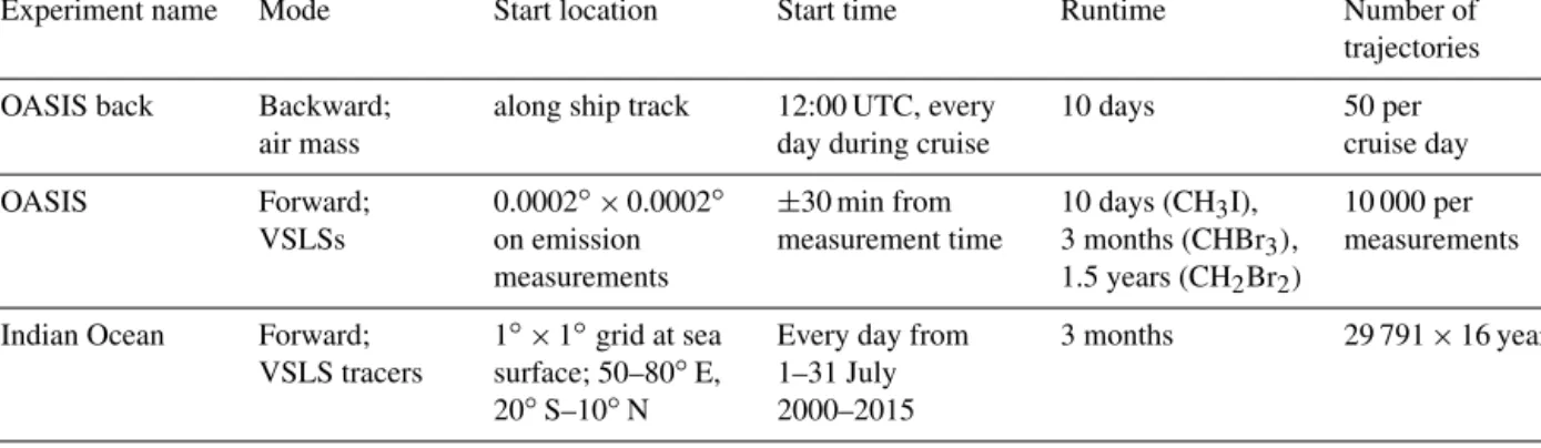
During the OASIS research cruise on RV Sonne in the subtropical and tropical West Indian Ocean in July and August 2014, the emissions of DMS, CH3I, CHBr3, and CH2Br2 were determined for the Indian Ocean. These are the first open Indian Ocean observations of CHBr3 and CH2Br2. In this thesis, the Lagrangian particle dispersion model Flexpart with ERA-Interim meteorological fields is used to simulate high resolution transport of oceanic emissions from the Indian Ocean to the stratosphere with different modeling approaches and for different regions, seasons, and years.
VSLS emissions from the tropical and subtropical West Indian Ocean to the stratosphere during Asian summer monsoon is investigated from 2000-2015. During OASIS in 2014, we observed average emissions of CH3I, high emissions of CHBr3, and very high emissions of CHBr2 in the subtropical and tropical West Indian Ocean, especially south of Madagascar and in the open ocean upwelling between 10˚S - S. The transport to the stratosphere is more efficient than above the tropical Atlantic, but less efficient than in the West Pacific during previous cruises. There are two main transport pathways from the West Indian Ocean to the stratosphere during the summer monsoon. The tropical deep convection around the equator is more relevant for the shorter-lived VSLS such as CH3I, while the monsoon convection over India and the Bay of Bengal and the Asian monsoon anticyclone transport mainly longer-lived VSLS like CHBr3 and CH2Br2 to the stratosphere. Over the 16 years, interannual variability and a small increase in transport through the Asian summer monsoon is found.
The second manuscript reports about DMS emission measurements with the eddy- covariance technique from the same Indian Ocean research cruise in July-August 2014.
The transport of DMS emissions in the troposphere and their influence on aerosol and cloud formation is investigated. A positive correlation between DMS emissions and satellite aerosol products indicate a local influence of marine DMS emissions on atmospheric aerosol formation, which impact the radiative budget.
After these two studies for the Asian summer season, the third manuscript considers the influence of the large seasonal differences of the Asian monsoon circulation.
Therefore, the intra- and interannual variability of transport from the tropical West Indian Ocean to the stratosphere and its causes is investigated from 2000-2015. The pronounced annual cycle of VSLS entrainment is driven by the shifting monsoon winds. The transport efficiency to the stratosphere is enhanced by high local sea surface temperatures in the tropical West Indian Ocean all year round. It can also be enhanced during boreal spring by El Niño events and during boreal fall by La Niña events in the central and eastern equatorial Pacific through changes in the Walker circulation. Intra- and interannual variability of transport efficiency to the stratosphere is larger for VSLS with shorter lifetimes.
Due to the pronounced annual cycle in transport efficiency found in the third paper, seasonal and regional variations in the VSLS emissions from the Indian Ocean are assumed to influence their stratospheric entrainment as well. Thus, the focus of the fourth
emissions on stratospheric delivery seasons and regions. This manuscript contains a process study for CHBr3 emissions and their transport from the tropical Indian Ocean and West Pacific to the stratosphere in 2014. The main oceanic source regions for stratospheric CHBr3 are the Bay of Bengal and the Arabian Sea during boreal summer.
The main stratospheric entrainment occurs during the same season over the southern tip of the Indian subcontinent. Using annual emissions, the highest CHBr3 volume mixing ratio at the tropopause is simulated above the tropical central Indian Ocean in boreal spring, while monthly emissions have a maximum in boreal summer in the Asian monsoon anticyclone. This seasonal and regional difference shows the importance of resolving seasonal and regional variations of emissions for the Indian Ocean in modeling efforts.
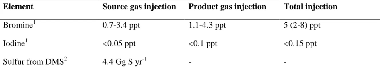
At the end of this thesis, I calculate the contribution of VSLS from the Indian Ocean to total tropical VSLS emissions from different emission inventories. The Indian Ocean contribution of the three VSLS CHBr3, CH2Br2, and DMS is higher than tropical averages, while CH3I emissions are slightly lower. Furthermore, the contribution of these emissions to total stratospheric bromine, iodine, and sulfur from VSLS is estimated. The relative contributions from the Indian Ocean to the stratospheric abundances are always higher than the tropical average contribution. The Indian Ocean is an important source region for VSLS to the troposphere and stratosphere because of high emissions and efficient upward transport through the Asian monsoon especially during boreal summer.
Anthropogene halogenierte Substanzen verursachen das Ozonloch über der Antarktis durch katalytische Ozonzerstörung und einen Schwund der stratosphärischen Ozonschicht, welche die Erde vor schadhafter ultravioletter Strahlung schützt. Seit 1989 reguliert das Montrealer Protokoll die Emissionen von langlebigen halogenierten Fluorchlorkohlenwasserstoffen. Seit dem Beginn des 21. Jahrhundert sinkt die atmosphärische Konzentration von Chlor und Brom aus den langlebigen anthropogenen Substanzen und das stratosphärische Ozon nimmt langsam wieder zu. Unter diesen Voraussetzungen wird die Bedeutung natürlicher halogenhaltiger Substanzen, vor allem sehr kurzlebiger Substanzen (engl. very short-lives substances, VSLS) mit atmosphärischen Lebenszeiten kürzer als ein halbes Jahr, für die Zusammensetzung und Chemie der Atmosphäre in der Zukunft zunehmen. Momentan beträgt der Beitrag von VSLS zum stratosphärischen Brom etwa 25%. Die beiden wichtigsten bromierten VSLS sind Bromoform (CHBr3, 17 Tage Lebenszeit) und Dibrommethan (CH2Br2, 150 Tage).
Weiterhin wird ein stratosphärischer Eintrag von Methyliodid (CH3I, 3,5 Tage) und schwefelhaltigem Dimethylsulfid (DMS, 1 Tag) vermutet. Schwefel verstärkt die heterogene chemische Ozonzerstörung bei hohem Chlorgehalt in der Stratosphäre. VSLS werden im Ozean auf natürlichem Wege von Phytoplankton, Makroalgen und durch chemische Reaktionen produziert. Sie werden in tropischen Gebieten mit hochreichender Konvektion in die Stratosphäre eingetragen, hauptsächlich über dem tropischen Westpazifik im borealen Winter und der asiatischen Monsunzirkulation im borealen Sommer. Die Unsicherheiten bezüglich der VSLS-Emissionen aus dem Indischen Ozean und des Transportes durch den asiatischen Monsun in die Stratosphäre sind groß. Diese Arbeit untersucht erstmalig VSLS Emissionen aus dem Indischen Ozean und ihren Transport in die Stratosphäre mit einer neuartigen Kombination aus Daten und Modellierung.
Während der OASIS Forschungsfahrt auf dem Forschungsschiff Sonne im subtropischen und tropischen westlichen Indischen Ozean im Juli und August 2014 wurden die Emissionen von CH3I und DMS und zum ersten Mal von CHBr3 und CH2Br2 im offenen Indischen Ozean ermittelt. In dieser Arbeit wird das Lagrangsche Partikeldispersionsmodell Flexpart mit ERA-Interim verwendet, um den hochaufgelösten
Modellansätzen und für verschiedene Regionen, Saisons und Jahre zu modellieren.
Im ersten Manuskript werden die Transportwege der halogenierten VSLS aus dem subtropischen und tropischen Westindik im asiatischen Sommermonsun zwischen 2000- 2015 bestimmt. Die aus den Messungen während OASIS in 2014 abgeleiteten Emissionen waren durchschnittlich für CH3I, hoch für CHBr3 und sehr hoch für CH2Br2, insbesondere südlich von Madagaskar und im ozeanischen Auftriebsgebiet zwischen 10˚S - 5˚S. Der Transport in die Stratosphäre ist effizienter als im tropischen Atlantik, aber weniger effizient als im Westpazifik währen vorhergehender Forschungsfahrten. Zwei Haupttransportwege in die Stratosphäre wurden durch die Simulationen diagnostiziert.
Die hochreichende tropische Konvektion um den Äquator ist wichtiger für den Transport des kurzlebigen VSLS CH3I, während die Monsunkonvektion über Indien und der Bucht von Bengalen und die asiatische Monsunantizyklone hauptsächlich die längerlebigen VSLS CHBr3 und CH2Br2 in die Stratosphäre transportieren. Die Eintragszeitserie zeigt interannuale Variabilität und einen leichten Anstieg der Transporteffizienz vom tropischen Westindik in die Stratosphäre über die 16 Jahre.
Im zweiten Manuskript werden DMS-Emissionsmessungen mit der Eddy-Kovarianz Methode von der gleichen Fahrt im Indik präsentiert. Der Transport der DMS-Emissionen in der Troposphäre während des Sommermonsuns und ihr Einfluss auf Aerosolbildung wird untersucht. Die positive Korrelation zwischen DMS-Emissionen und Aerosolprodukten von Satellitenmessungen bestätigt den lokalen Einfluss von marinen Spurengasen auf atmosphärische Aerosole.
Nachdem die ersten beiden Studien lediglich den Transport während der borealen Sommermonate betrachten, beschäftigt sich das dritte Manuskript mit den Einflüssen der starken saisonalen Unterschiede in der asiatischen Monsunregion. Hier werden die intra- und interannuale Variabilität des Transportes vom tropischen Westindik in die Stratosphäre und ihre Ursachen im Zeitraum von 2000-2015 untersucht. Es gibt, einen ausgeprägten Jahresgang im stratosphärischen Eintrag getrieben von den wechselnden Monsunwinden. Die Transporteffizienz in die Stratosphäre wird das ganze Jahr über durch hohe lokale Meeresoberflächentemperaturen im tropischen Westindik verstärkt. Im borealen Frühling wird der Eintrag außerdem durch El Niño- und im borealen Herbst durch La Niña-Verhältnisse im zentralen und östlichen äquatorialen Pazifik intensiviert.
Die intra- und interannuale Variabilität der Transporteffizienz in die Stratosphäre ist höher je kürzer die Lebenszeit der VSLS ist.
der Emissionen aus dem Indischen Ozean auch den stratosphärischen Eintrag beeinflussen. Deshalb liegt der Fokus des vierten Manuskriptes auf den Auswirkungen von jährlich und monatlich aufgelösten VSLS Emissionen auf die Saison und Region des Eintrages in die Stratosphäre. Das Manuskript enthält eine Prozessstudie für CHBr3- Emissionen aus dem tropischen Indik und Westpazifik und ihren Transport in die Stratosphäre in 2014. Das in die Stratosphäre eingetragene CHBr3 kommt im borealen Sommer hauptsächlich aus der Bucht von Bengalen und dem Arabischen Meer. Der Eintrag in die Stratosphäre aus dem tropischen Indischen Ozean und Westpazifik ist über der südlichen Spitze von Indien konzentriert, ebenfalls im borealen Sommer. Werden jährliche Emissionen verwendet, so sind die simulierten CHBr3 Mischungsverhältnisse an der Tropopause im borealen Frühling am höchsten. Monatliche Emissionen führen zu einem Maximum der Mischungsverhältnisse in der asiatischen Monsunantizyklone im borealen Sommer. Dieser saisonale und regionale Unterschied zeigt die Bedeutung der saisonalen und regionalen Auflösung der Emissionen aus dem tropischen Indischen Ozean für Modellstudien.
Am Ende der Doktorarbeit berechne ich den Beitrag der VSLS Emissionen aus dem tropischen Indischen Ozean zu den gesamten tropischen Emissionen aus verschiedenen Emissionsinventaren. Der Beitrag des Indik zu Emissionen der drei VSLS CHBr3, CH2Br2 und DMS ist höher als im tropischen Mittel, während CH3I Emissionen etwas weniger als im Durchschnitt beitragen. Ich schätze außerdem den Beitrag dieser Emissionen zum gesamten stratosphärischen Brom, Iod und Schwefel aus VSLS ab. Der relative Beitrag des Indischen Ozeans zu stratosphärischen Konzentrationen ist für alle VSLS höher als der mittlere tropische Beitrag. Der Indische Ozean ist eine wichtige Quellregion für VSLS für die Troposphäre und Stratosphäre aufgrund der starken Emissionen und dem effizienten Transport in die Stratosphäre durch den Asiatischen Monsun besonders im borealen Sommer.
This thesis is based on the following manuscripts:
1. Manuscript 1: Delivery of halogenated VSLS to the stratosphere
Fiehn, A.; Quack, B.; Hepach, H.; Fuhlbrügge, S.; Tegtmeier, S.; Toohey, M.; Atlas, E.; and Krüger, K.: Delivery of halogenated very short-lived substances from the west Indian Ocean to the stratosphere during the Asian summer monsoon, Atmos.
Chem. Phys., 17, 6723-6741, https://doi.org/10.5194/acp-17-6723-2017, 2017.
My contribution: I designed the model experiments together with K. Krüger and B.
Quack and I carried them out. I was involved in the VSLS measurements and analyses made during the OASIS cruise. I analyzed and interpreted the meteorological cruise date. I prepared the manuscript with help from K. Krüger and B. Quack with contributions from all co-authors.
2. Manuscript 2: The influence of air-sea fluxes on atmospheric aerosols
Zavarsky, A.; Booge, D.; Fiehn, A.; Krüger, K.; Atlas, E.; and Marandino, C.: The influence of air-sea fluxes on atmospheric aerosols during the summer monsoon over the Indian Ocean, under review at Geophysical Research Letters.
My contribution: I calculated the air mass back- and forward trajectories with Flexpart/ERA-Interim and helped writing and reviewing the manuscript.
3. Manuscript 3: Variability of VSLS transport to the stratosphere
Fiehn, A.; Quack, B.; Marandino, C. A.; Krüger, K.: Variability of VSLS transport from the West Indian Ocean to the stratosphere, under review at Journal of Geophysical Research: Atmospheres.
My contribution: I designed the model simulations with help from all co-authors and carried them out. I analysed the model data and wrote the manuscript with contributions from all co-authors.
4. Manuscript 4: Influence of seasonally resolved emissions
Fiehn, A.; Quack, B.; Stemmler, I.; Ziska, F.; and Krüger, K.: Influence of seasonally resolved emissions on the transport of bromoform from the Indian Ocean to the stratosphere, Atmos. Chem. Phys., in preparation.
My contribution: I created the emission fields with advice from B. Quack. All co- authors designed the model experiments and I carried out the FLEXPART
contributions from all co-authors.
In addition, I contributed to the following publication through dispersion modelling with Flexpart:
Fuhlbrügge, S., Quack, B., Atlas, E., Fiehn, A., Hepach, H., and Krüger, K.:
Meteorological constraints on oceanic halocarbons above the Peruvian upwelling, Atmos.
Chem. Phys., 16, 12205-12217, https://doi.org/10.5194/acp-16-12205-2016, 2016.
1 Introduction ... 3
1.1 Asian monsoon and the Indian Ocean ... 5
1.1.1 General circulation of the atmosphere ... 5
1.1.2 Asian monsoon circulation ... 7
1.1.3 Asian monsoon variability and trends ... 10
1.1.4 Transport of surface air to the stratosphere through the Asian monsoon ... 14
1.1.5 Indian Ocean circulation ... 17
1.2 Very short-lived substances and their transport to the stratosphere ... 18
1.2.1 Marine production ... 18
1.2.2 Air-sea gas exchange ... 19
1.2.3 VSLS emission estimates ... 21
1.2.4 Atmospheric degradation and lifetimes... 23
1.2.5 VSLS entrainment to the stratosphere ... 24
1.2.6 Impacts of VSLS on the stratosphere ... 26
2 Research Questions ... 29
3 Results ... 33
3.1 Manuscript 1 ... 33
3.2 Manuscript 2 ... 65
3.3 Manuscript 3 ... 85
3.4 Manuscript 4 ... 129
4 Summary, Conclusions, and Outlook ... 173
5 References ... 183
6 List of Figures ... 195
7 List of Tables ... 197
8 List of Abbreviations ... 199
Curriculum Vitae ... 203
Danksagung... 205
Eidesstattliche Erklärung ... 207
The ozone hole above Antarctica was first discovered in 1984 (Chubachi, 1984; Farman et al., 1985). It occurs in southern hemispheric spring and is connected with catalytic depletion of the stratospheric ozone layer involving anthropogenic chloro- and bromofluorocarbons (Molina et al., 1974; Wofsy et al., 1975). The stratospheric ozone layer protects the Earth’s surface from harmful ultraviolet (UV) radiation originating from the sun. This radiation impacts physiological and developmental processes in plants and increases the incidence of skin cancer, eye diseases, and infectious diseases in humans and animals (Van der Leun et al., 1995). Anthropogenic ozone depleting substances (ODS) cause a reduction of the stratospheric ozone abundances which is small around the equator, larger in the midlatitudes and most pronounced at the poles in spring.
ODS have been widely used as refrigerants, propellants, solvents, extinguishers, fumigants, and cleaning agents before they were banned when the Montreal Protocol entered into force in 1989. Because of the long lifetimes of the major chlorofluorocarbons (CFC-11 around 50 years, CFC-12 around 100 years), their abundances in the atmosphere are decreasing slowly and a recovery of the global ozone level to 1960 values is projected for approximately the middle of the 21st century (WMO, 2014).
Beside the depletion of the ozone layer by ODS, there is also a contribution of natural chlorinated, brominated, and iodinated substances to ozone destruction. Bromine is important for ozone chemistry despite much lower stratospheric abundances than chlorine, since it is about 60 times more efficient at destroying ozone than chlorine (Sinnhuber et al., 2009). Iodine is more than 100 times as efficient as chlorine in depleting ozone (Ko et al., 2003). The impact of natural long-lived halogenated substances, mainly methyl chloride (CH3Cl) and methyl bromide (CH3Br), on the ozone layer is relatively well known (WMO, 2014). The role of shorter-lived bromine containing compounds in ozone depletion is, however, less certain. Recent balloon-borne stratospheric bromine measurements revealed a discrepancy between measured bromine abundances and those, that could be accounted for by long-lived gases (Dorf et al., 2006). The missing stratospheric bromine source is attributed to natural marine derived substances with lifetimes in the order of days to half a year, which are called very short-lived substances (VSLS) (Law et al., 2006). The two natural oceanic compounds bromoform (CHBr3) and dibromomethane (CH2Br2) are estimated to contribute ~76% to VSLS bromine ( )
in the stratosphere using a top down approach (Hossaini et al., 2012). The natural oceanic VSLS methyl iodide (CH3I) delivers small amounts of iodine to stratosphere, when it is emitted in regions with active convection (Solomon et al., 1994; Tegtmeier et al., 2013).
Polar ozone depletion occurs by heterogeneous reactions involving chlorine on the surface of polar stratospheric clouds, which mainly consist of sulfuric acid aerosols (Solomon et al., 2015). These aerosols are also the major constituents of the stratospheric background aerosol layer (Junge et al., 1961), which impacts Earth’s radiative budget by cooling the surface climate (Solomon et al., 2011). The stratospheric background aerosol layer is supplied by long-lived natural substances from the ocean e.g. carbonyl sulfide (Crutzen, 1976; Kremser et al., 2016) and anthropogenic sulfur compounds such as sulfur dioxide (Myhre et al., 2004; Solomon et al., 2011; Sheng et al., 2015). Volcanic eruptions can significantly contribute to stratospheric sulfur (Mossop, 1964) over timescales of a few months to years. Oceanic DMS, the major biogenic sulfur carrier to the atmosphere (Liss et al., 2014), may despite its very short lifetime of around one day directly contribute to stratospheric sulfur in regions of pronounced tropical deep convection like the tropical West Pacific (Marandino et al., 2013). Furthermore, it contributes through the atmospheric conversion to carbonyl sulfide (Barnes et al., 1994) and subsequent entrainment to the stratosphere.
These very short-lived halogen and sulfur containing substances are naturally produced by phytoplankton and macroalgae (Moore et al., 1994; Carpenter et al., 1999;
Stefels, 2000; Quack et al., 2003) and are emitted to the atmosphere when they are oversaturated in the surface ocean. The emissions of VSLS vary spatially and temporally and depend on the concentrations in ocean and atmosphere, as well as on physical parameters like sea surface temperature, salinity, and wind speed (Quack et al., 2003).
VSLS are mainly transported to the stratosphere through fast uplift with deep convection in the tropics. The main entrainment regions of tropospheric air to the stratosphere, the so-called “stratospheric fountain”, are the Pacific warm pool in boreal winter and the Asian monsoon in boreal summer (Newell et al., 1981). After entering the stratosphere, air is transported from the tropics toward the winter pole with the Brewer-Dobson circulation (Brewer, 1949; Dobson, 1956). Tropical oceanic surface sources of VSLS matter for the ozone cycle in the atmosphere and ozone depletion in midlatitudes and polar regions of the stratosphere (Oman et al., 2016; Fernandez et al., 2017).
Major uncertainties still exist with regard to the sources and strength of the highly variable VSLS emissions from the oceans and their transport to the stratosphere.
Especially emissions from the Indian Ocean, which is the most rapidly warming ocean basin in current climate change (Roxy et al., 2014), are poorly constrained due to very sparse data coverage in this ocean basin (Lana et al., 2011; Ziska et al., 2013).
Furthermore, the Asian monsoon as important gateway for tropospheric air to the stratosphere (Fueglistaler et al., 2005) has not been studied in detail as a VSLS pathway with observations or models. Thus, it is important to investigate the emissions and transport processes of VSLS in the Asian monsoon region in order to calculate the contribution of natural halocarbons and sulfur under present-day conditions. Only by understanding the current situation can we begin to predict the influence of these natural compounds on the stratosphere in a future climate, which will likely include a slowing of the Asian monsoon circulation (Christensen et al., 2013).
The relative importance of natural halogenated compounds for ozone depletion will change in the future since the stratospheric chlorine abundances are declining due to the regulation of ODS emissions through the Montreal protocol. The ozone depletion efficiency of bromine will decrease with the future stratospheric abundance of chlorine and thus the chlorine-bromine ozone destruction cycle will become less efficient (Yang et al., 2014). Taking this depletion efficiency decrease into account, Tegtmeier et al. (2015) projected the ozone depletion potential of CHBr3 to increase until 2100 due to enhanced emissions and larger convective mass flux. Furthermore, the emissions of CHBr3 are projected to increase, if oceanic concentrations remain the same (Ziska et al., 2017).
However, it is unclear what will happen to ocean concentrations in a future climate, as they depend on oceanic biological activity (Stemmler et al., 2015). The impact of future climate scenarios on oceanic biology is highly debated (Richardson et al., 2016; Roxy et al., 2016). Thus, projections of future VSLS influence on ozone are still inconclusive and detailed emission and transport studies are needed to reduce the existing uncertainties.
1.1 Asian monsoon and the Indian Ocean
1.1.1 General circulation of the atmosphere
The general circulation of the atmosphere depicts the mean global flow in the atmosphere averaged with time. The circulation is driven by the differential heating from the sun between the equator and the poles and further influenced by the rotation of the earth and the distribution of continents and oceans. The difference in incoming solar energy
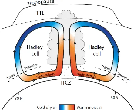
between the equator and the poles causes a surface pressure gradient with low pressure at the equator and high pressure at the poles. This gradient accelerates surface air parcels towards the equator. They are deflected to the right on the northern hemisphere and to the left on the southern hemisphere due to the Coriolis effect, a result of the rotation of the earth and their movement away from the rotation axis. The movement toward the equator of surface air is interrupted by the deflected air masses in the midlatitudes, where westerly winds prevail. A circulation cell, called the Hadley cell, exists between the equator and the subtropics on each hemisphere (Figure 1). In these cells air parcels rise around the equator, flow towards the poles in the upper troposphere, descend in the subtropics and converge toward the center at the surface. The resulting tropical easterly winds at the surface are the trade winds and the temperature inversion occurring due to the descending air masses is called trade inversion. The low pressure center, called the intertropical convergence zone (ITCZ), is marked by rising air masses and intense rainfall.
The position of the ITCZ and the accompanying rainfall shift over the year as the latitude of maximum incoming solar radiation moves towards the summer hemisphere of the Earth. On average, it is located around 5˚N, but over the Indian Ocean its mean position is south of the equator (Schneider et al., 2014).
Figure 1: Schematic of the Hadley circulation. Abbreviations: TTL – Tropical tropopause layer, ITCZ – Intertropical convergence zone.
1.1.2 Asian monsoon circulation
The Asian monsoon dominates the atmospheric circulation above the Indian Ocean. The term monsoon refers to a seasonal shift in the prevailing surface winds. This shift is often accompanied by a change in the precipitation regime from a rainy season with onshore flow to a dry season with offshore flow (Krishnamurti et al., 2013). Ramage (1971) defined monsoon regions by a shift in the surface winds of at least 120° between January and July. More recent definitions include a local difference between summer and winter precipitation (called annual range; Wang et al., 2006; Figure 2) and the normalized seasonality in the wind field (Li et al., 2003). The monsoon has been described as a global-scale persistent overturning of the atmosphere that varies with the time of year (Trenberth et al., 2000). It can be divided into three regional monsoons, which are summarized under the term global monsoon: The American, the African, and the Asian- Australian monsoon.
Figure 2: Annual range (difference between summer and winter precipitation) and global monsoon domain (delineated by the bold line) after the definition of Wang et al. (2006).
Webster (1987) suggested the monsoon to be a planetary scale moist sea-breeze modified by the Coriolis force. Satellite observations showed that the monsoon is also part of the planetary rain band connected with the ITCZ, only the amplitude of displacement from the equator is larger in monsoon regions (Sikka et al., 1980).
Seasonally reversing winds are associated with large-scale heat sources and sinks. The Asian summer monsoon heat source first comes from the warm Indian subcontinent and is then intensified by the heavy rainfalls over India, Indochina, and China and the associated convective heating. Additionally, the elevated grounds of the Tibetan Plateau
absorb solar radiation and release it back into the atmosphere through sensible and latent heat fluxes above the sea level, meaning that the large-scale meridional temperature gradient also exists over significant depth in the troposphere. The boreal summer heat sink lies in the southern Indian Ocean between 30˚S and 60˚S and the southern part of the South China Sea (Krishnamurti et al., 2013). The temperature difference creates the Monsoon Low pressure system on the Asian continent and the Mascarene High above the ocean (Figure 3). The seasonal displacement of the ITCZ is amplified by these pressure systems. The global monsoons mainly respond to the net heating on planetary scales, but the regional monsoons depend on the distribution of land and ocean, as well as sea surface temperature (SST) gradients and topography (Webster, 1987). The uneven distribution of land and ocean between northern and southern hemisphere and the high altitude of the Himalaya create a pressure gradient that makes the Asian monsoon the most pronounced monsoon. The Asian monsoon is often divided into the Indian monsoon, also called South Asian monsoon, and the East Asian monsoon. These monsoons are two separate but interactive monsoon sub-systems (Wang et al., 2001).
The Indian summer monsoon surface winds develop above the southern Indian Ocean as southeast (SE) trades, flow across the equator and onto the Indian subcontinent as the Somali Jet and southwest (SW) monsoon, bringing moisture toward the convective centers over northern India and the Bay of Bengal (Figure 3).
Figure 3: Schematic of the major circulation of the surface winds, the Hadley cell, and the jets of the Indian summer monsoon (after Meehl, 1987).
The release of latent heat from the convection establishes an upper tropospheric high pressure system with anticyclonic circulation above the Asian continent (Figure 4a). This pressure system, called Asian monsoon anticyclone, is flanked by the subtropical jet in the north and the Tropical Easterly Jet (TEJ) in the south (Dunkerton, 1995) (Figure 4b).
Figure 4: ERA-Interim monthly fields for July 2014 at 100 hPa for (a) geopotential height anomaly with wind arrows and (b) zonal wind speed with geopotential height anomaly contours. Abbreviations: Asian monsoon anticyclone (AMA), subtropical jet (SJ), Tropical Easterly Jet (TEJ).
The winter monsoon over Asia is characterized by northeasterly offshore winds both in India and East Asia and little rainfall over the continents. The ITCZ and accompanying rainfall over the Indian Ocean is located to the south of the equator. Figure 5 depicts the annual movement of main precipitation over the Indian Ocean. Note that some deep convection and rain remains around the equator, when the main convection center moves to the northern hemisphere in boreal summer.
Figure 5: Annual shift of main rainfall and surface winds over the Indian Ocean. The red line marks the ITCZ (precipitation maxima) (Schneider et al., 2014).
1.1.3 Asian monsoon variability and trends
The Asian monsoon experiences variability on different time scales, from intraseasonal over interannual to inter-decadal and additionally long-term trends driven by changes and variability in the oceans and the atmospheric circulation. This thesis determines the seasonal and interannual variability in transport of VSLS from the ocean to the stratosphere via the Asian monsoon circulation. The seasonal variability is mainly driven by the strong annual cycle of the Asian monsoon. Interannual variability in the Asian monsoon exists and is connected to other oceanic or atmospheric phenomena acting on interannual scales in the tropics. Furthermore, this thesis briefly investigates short-term (15-year time period) changes in transport to the stratosphere, which may be caused by changes in the monsoon circulation and its drivers. These changes may impact the stratospheric delivery of VSLS and, thus, influence stratospheric composition and chemistry.
The variability of the Asian monsoon is expressed by certain physical parameters like rainfall and wind speed at different locations or heights. Some of the most important indices for the Asian and Indian monsoon are:
All-India Rainfall Index (AIRI): sum of rainfall over the Indian continent during June to September (Parthasarathy et al., 1994),
Extended Indian monsoon rainfall (EIMR): sum of rainfall including adjacent oceans covering 70˚–110˚E, 10˚–30˚N during June to August,
Webster Yang Index (WYI): broad-scale South Asian summer monsoon index, vertical shear of zonal wind anomalies between 850 hPa and 200 hPa during JJA, (40˚–110˚E, 0˚–20˚N) defined in Webster et al. (1992),
Indian Monsoon Index (IMI): dynamical index for the Indian monsoon, horizontal shear of zonal wind between a southern region (40˚–80˚E, 5˚–15˚N) and a northern region (70˚–90˚E, 20˚–30˚N) at 850 hPa (Wang et al., 1999;
Wang et al., 2001).
In my thesis, I use the AIRI and IMI to investigate seasonal variability of atmospheric transport through the Indian monsoon. The characteristics of a pronounced Indian summer monsoon include a strong Mascarene high over the southern subtropical Indian Ocean, a distinct land-sea thermal gradient and a resulting enhanced cross-equatorial flow with increased moisture transport towards India (Webster et al., 2003).
Interannual variability in the tropics, especially the Indian and Pacific Ocean, is modulated by coupled ocean-atmosphere phenomena. These often also influence each other. The phenomena discussed here are the El Niño-Southern Oscillation (ENSO), the Indian Ocean Dipole (IOD), the Tropospheric Biennial Oscillation (TBO), and the Pacific Decadal Oscillation (PDO). A map of the areas, where indices for these phenomena and the IMI are defined, can be found in Manuscript 3 (Sect. 3.3).
El Niño-Southern Oscillation (ENSO)
The main interannual influence on the Asian monsoon is through ENSO (Webster et al., 1992; Ju et al., 1995) (Figure 6). It is a coupled ocean-atmosphere phenomena in the equatorial Pacific, with remote influences around the globe. The easterly trade winds over the Pacific push warm surface waters towards the west inducing an SST gradient of about 5˚C between the West Pacific warm pool and the East Pacific. The movement of water mass also causes sea level differences around 0.5 m between the east and the west, an inclination of the thermocline, the border between warm surface and cold bottom water, and upwelling of cold bottom water along the South American coast. This upwelling is increased by the offshore Ekman transport induced by the southerly winds along the South American coast. The equatorial easterly winds above the Pacific are part of the atmospheric Walker circulation (Walker, 1924). It is an earth encompassing zonal circulation in the tropics with atmospheric upwelling over the warm continents, downwelling over the oceans, and compensating horizontal easterly or westerly winds at the surface and in the upper troposphere.
Figure 6: (a) West Pacific SST, Walker cell and upwelling during ENSO neutral conditions. (b) West Pacific SST anomalies, Walker cells and reduced upwelling during El Niño conditions (Christensen et al., 2013).
The state of the Pacific Ocean is sustained by the positive Bjerknes feedback (Bjerknes, 1969): The SST difference across the equatorial Pacific limits convection to the West Pacific, which creates a pressure gradient strengthening the easterly winds. The variation of the pressure gradient between the East and the West Pacific is called the Southern Oscillation and is the atmospheric part of the coupled phenomena. Perturbations to this ocean-atmosphere feedback weaken the whole system and cause large variability known as ENSO. If, for example, the trade winds are weakened due to westerly wind bursts originating in the Indian Ocean, less water is displaced to the West Pacific, the East Pacific warms and the oceanic upwelling along the South American coast is reduced. This is called an El Niño (Spanish: Christ Child) event, because it is observed around Christmas time in boreal winter. The opposite event (La Niña, the girl) supports stronger than normal trade winds, lower temperatures in the East Pacific and enhanced oceanic upwelling. El Niño events occur every 3-7 years and can be described by SST anomalies in the equatorial Pacific in different regions (Nino3: 150˚–90˚W, 5˚S–5˚N; Nino4: 160˚E–
150˚W, 5˚S–5˚N). The influence of ENSO on the Asian monsoon is mainly through its modulation of the Walker circulation (Ju et al., 1995; Wang et al., 2001, Figure 6, Manuscript 3), but also due to a basin wide warming during El Niño in the adjacent Indian Ocean (Schott et al., 2009). For the Indian monsoon, a developing El Niño generally means less summer monsoon rainfall and vice versa for La Niña (Wang et al., 2001) (Figure 7). This connection and its influence on VSLS transport to the stratosphere are described in more detail in Manuscript 3 (Sect. 3.3).
Figure 7: Time series of All-Indian Summer (JJA) monsoon rainfall and ENSO events (Kothawale et al., 2016).
Indian Ocean Dipole (IOD)
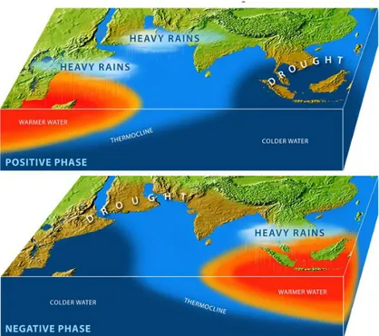
The IOD describes the SST anomaly between the West and East Indian Ocean, which has been shown to influence convection and rainfall in that basin (Figure 8). The Dipole Mode Index (DMI), used to describe the IOD, is defined as the SST difference between a western (50˚E-70˚E, 10˚S-10˚N) and an eastern (90˚E-110˚E, 10˚S-0˚) area in the Indian Ocean (Saji et al., 1999). A positive IOD event (a colder eastern Indian Ocean) during boreal summer suppresses deep convection in that region, enhances northward moisture transport toward the monsoon convection and causes more monsoon rainfall (Behera et al., 1999; Ashok et al., 2001).
The tropical circulation has the tendency that a relatively strong Indian monsoon is followed by a relatively weak one, and vice versa. This phenomena is called the Tropical Biennial Oscillation (TBO, Meehl et al., 2002). ENSO, the IOD, and the TBO are all tied together by the Walker circulation over the Indian and Pacific Ocean in the atmosphere (Meehl et al., 2002). The Pacific Decadal Oscillation describes the recurring SST pattern in the Pacific, with anomalies poleward of 20˚N (Mantua et al., 2002). On a longer than interannual time scale, the PDO has a similar impact on the Indian summer monsoon rainfall as ENSO, with a negative PDO phase related to an increase in summer monsoon rainfall and vice versa (Krishnan et al., 2003).
Figure 8: Sea surface temperature anomalies and rainfall patterns during positive and negative Indian Ocean Dipole events (Illustration by Paul E. Oberlander, 2017, Woods Hole Oceanographic Institution).
The Asian monsoon circulation has experienced long-term changes due to greenhouse gas induced global warming in the last decades (Christensen et al., 2013). The Indian Ocean has been warming for over a century, at a rate faster than any other ocean basin (Roxy et al., 2014). This warming decreases the land-sea thermal gradient, which drives the Indian monsoon, and thus slows down the monsoon circulation as observed from 1905-2012, resulting in less rainfall over the central-east and northern regions of India (Roxy et al., 2015). This decrease in rainfall is part of a dipole structure with an increase over the core monsoon region of Pakistan caused by more northward moisture transport over the Arabian Sea and less over the Bay of Bengal from 1951-2012 (Latif et al., 2016).
These changes could be due to a 2˚-3˚ westward shift of the whole Asian monsoon circulation system between 1970 and 2015 (Preethi et al., 2016). These recent studies also report a slowing down of the circulation over the Bay of Bengal, which could result in less convection and upward transport.
1.1.4 Transport of surface air to the stratosphere through the Asian monsoon
The delivery of surface air to the stratosphere depends on fast vertical transport, which is mainly realized in enhanced deep convection in the tropics. Generally air masses are lifted into the lower tropical tropopause layer (TTL) through convective processes and then ascend more slowly through the upper part of the TTL into the stratosphere (Figure 9, Path #3). The TTL is a layer of transition between the convective troposphere and the slow ascent of the Brewer-Dobson circulation in the stratosphere. Different definitions for the TTL exist (Folkins et al., 1999; Gettelman et al., 2002; Fueglistaler et al., 2009;
Carpenter et al., 2014). Here, the definition as the layer between the level of maximum convective outflow (~12 km altitude, 345 K potential temperature) and the cold-point tropopause (CPT, ~17 km, 380K) is used (Carpenter et al., 2014). The level of zero radiative heating (LZRH) marks the transition from clear-sky radiative cooling to clear- sky radiative heating and the boundary between the lower and upper TTL. Deep convection rapidly transports boundary level air masses up to the level of maximum convective outflow, typically between 12 and 14 km (Folkins et al., 2005). Air masses that are detrained below the LZRH mostly descend back into the mid-troposphere with the large-scale subsidence (Figure 9, Path #2). Air detrained above the LZRH can ascend through the upper TTL and reach the stratosphere. The residence time in the upper TTL
for northern hemispheric winter lies within 15-75 days (Krüger et al., 2009). The residence times in the TTL vary in space and time and are influenced by the location of entry and the horizontal transport through upwelling and downwelling regions (Tzella et al., 2011; Bergman et al., 2012). Overshooting deep convection that transports air masses directly above the tropopause essentially reduces residence times in the TTL (Pommereau, 2010). However, the contribution of this transport pathway to troposphere-to-stratosphere transport is still uncertain (Liu et al., 2005; Vernier et al., 2011; Takahashi et al., 2014).
Additionally, horizontal two-way exchange between the TTL and the extratropical lower stratosphere is also possible (Holton et al., 1995; Levine et al., 2007; Ploeger et al., 2012).
Figure 9: Schematic of vertical transport pathways in the tropics (Bergman et al., 2012).
Preferred regions of air mass transport to the stratosphere appear in conjunction with strong and fast convection above the Maritime Continent in boreal winter (Bergman et al., 2012), the Indian monsoon region (Devasthale et al., 2010) and Southeast Asia (Wright et al., 2011) in boreal summer. Above the tropical Indian Ocean, transport to the stratosphere is strongly influenced by the Asian monsoon circulation and its seasonality and interannual variability.
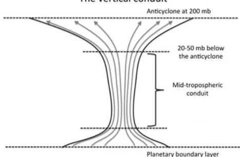
Stratospheric entrainment of boundary layer trace gases and volcanic aerosols has been detected in connection with the Asian monsoon (Randel et al., 2010; Bourassa et al., 2012). Chemistry climate models support the importance of this pathway for stratospheric delivery (Pan et al., 2016). The Asian monsoon anticyclone in the upper troposphere/lower stratosphere (UTLS) confines boundary layer air masses that have been lifted with the monsoon convection (Park et al., 2009). Furthermore, boundary layer source regions of anticyclonic air have been a topic of recent research. Bergman et al.
(2013) identified a slender mid tropospheric vertical conduit connecting India and the
Tibetan Plateau with the anticyclone. The importance of deep convective updrafts for the delivery to the tropopause was identified (Figure 10). This conduit is very persistent and efficient during the Asian summer monsoon. Chen et al. (2012) found the west Pacific Ocean and the Bay of Bengal to be important boundary layer sources for stratospheric entrainment in the Asian summer monsoon area. Vogel et al. (2015) showed that different boundary source regions contribute to the anticyclone related to intraseasonal variation of the summer monsoon associated with the north-south movement of the anticyclone.
Figure 10: The vertical conduit of boundary layer air masses to the Asian monsoon anticyclone (after Bergman et al., 2013).
From the anticyclone, air masses can be entrained into the stratosphere via slow vertical lifting in the tropics or through quasi-isentropic two way entrainment into the extratropical lowermost stratosphere (Vogel et al., 2015; Garny et al., 2016; Müller et al., 2016). A Lagrangian transport model driven by ERA-Interim inferred that Asian monsoon anticyclonic air contributes up to 5% of the air mass fraction in the confined tropical upwelling in the stratosphere, called the tropical pipe, and 15% to the extratropical lowermost stratosphere (Ploeger et al., 2017).
The boreal winter season is less important for stratospheric entrainment through the Asian monsoon than the summer monsoon season (Pan et al., 2016). The ITCZ resides slightly south of the equator over the Indian Ocean during this time (Schneider et al., 2014). The convection during this season is weaker, but directly over the Indian Ocean, a potential source region for VSLS.
1.1.5 Indian Ocean circulation
The interaction of the tropical Indian Ocean with the atmosphere plays an important role in shaping climate on regional and global scales. The Indian Ocean differs from the Atlantic and Pacific Oceans in several aspects, including the northward boundary of the Asian continent and the low latitude exchange of ocean waters with the Pacific through the Indonesian Through Flow (ITF, Figure 11). The Indian Ocean and the Asian continent drive the strongest monsoon in the world, which exerts an important impact on the Indian Ocean seasonal cycle through a reversal of the monsoon winds.
The Indian Ocean lacks the steady equatorial easterly winds that occur over the Atlantic and Pacific. As a result, there is, in contrast to the other oceans, no climatological mean equatorial upwelling along its eastern boundary. Instead, upwelling occurs along the coast of Africa and Arabian Peninsula, maybe east and west of the tip of India, and south of the equator in the West Indian Ocean (green in Figure 11). These upwelling regimes are connected to the shallow “equatorial roll”, which does not exist in other oceans. During the summer monsoon, this roll emerges from the mean southward Ekman transport across the tropical Indian Ocean (red arrows in Figure 11).
Figure 11: Indian Ocean currents during boreal summer partaking in the equatorial roll circulation and areas of upwelling (green shading) and downwelling (blue shading). Light dashed stream paths stand for upper layer inflow into downwelling area, dotted for thermocline Somali Current supply, solid for Southern Hemisphere thermocline flow, and heavy dashed for the supply route of the subtropical cell.
Abbreviations: Indian Through Flow (ITF), Southern Equatorial Current (SEC), Northeast Madagascar Current (NEMC), East African Coastal Current (EACC), South Equatorial Counter Current (SECC), Somali Current (SC), Great Whirl (GW), Mean Ekman Transport (Me) (Schott et al., 2009).
The wind stress is directed to the north along the equator causing the Ekman driven current to subduct and form the equatorial roll. The water wells up again south of the equator forming the Seychelles-Chagos-thermocline ridge (Schott et al., 2009).
Furthermore, the atmospheric Somali Jet of the Asian summer monsoon causes strong coastal upwelling of bottom water along the Somali coast (Bruce, 1973).
1.2 Very short-lived substances and their transport to the stratosphere
VSLS are gases that have atmospheric lifetimes of less than half a year after they have been emitted to the atmosphere (Law et al., 2006). This thesis focuses on the four VSLS bromoform (CHBr3), dibromomethane (CH2Br2), methyl iodide (CH3I) and dimethyl sulfide (DMS).
1.2.1 Marine production
The four VSLS discussed in this thesis have their main sources in the oceans. The production of bromocarbons in the ocean is not yet fully understood, but production pathways have been identified. The two bromocarbons CHBr3 and CH2Br2 have biological and chemical production pathways. Macroalgal formation of bromocarbons has been investigated in the field and laboratory (Gschwend et al., 1985; Carpenter et al., 2000). There is also a source of bromocarbons from phytoplankton in the open ocean (Quack et al., 2004). Several phytoplankton pigments and groups have been related to CHBr3 and CH2Br2 production (Moore et al., 1995b; Quack et al., 2007; Hughes et al., 2013), while they are poor proxies for bromocarbon production (Abrahamsson et al., 2004; Ordóñez et al., 2012; Stemmler et al., 2015). Incubation studies of phytoplankton confirmed the production of bromocarbons from bromoperoxidase enzymes (Tokarczyk et al., 1994; Moore et al., 1996). Furthermore, anthropogenic sources of CHBr3 and CH2Br2 need to be considered. The compounds are formed during the chlorination and ozonization of drinking, sea, and waste water for disinfection and cooling water in power plants to prevent biofouling (Fogelqvist et al., 1982; Fogelqvist et al., 1991; Jenner et al., 1997). Generally, the sources can be divided in coastal and open ocean sources, with macroalgae and anthropogenic production dominating the coastal sources, which yield higher concentrations than phytoplankton in the open ocean (Quack et al., 2003).
For CH3I production, small biological sources were detected from kelp macroalgae (Lovelock, 1975; Gschwend et al., 1985), phytoplankton (Moore et al., 1996; Scarratt et al., 1999), and bacterial production (Amachi et al., 2001; Hughes et al., 2011). Through incubation experiments also a photochemical source of CH3I was detected (Moore et al., 1994; Shi et al., 2014). The inclusion of photochemical production in the ocean closed the gap in the global atmospheric CH3I budget (Bell et al., 2002).
DMS is formed in the ocean from its precursor dimethylsulfoniopropiate (DMSP), which is produced by phytoplankton (Stefels, 2000). DMSP is released to the water and about 1-10% degrades enzymatically into DMS (e.g. Bates et al., 1994; Liss et al., 2014).
The production of DMS has been studied in the field (e.g. Simó et al., 2002) and modeled with biogeochemical coupled ocean atmosphere models (e.g. Kloster et al., 2006).
1.2.2 Air-sea gas exchange
Air-sea gas exchange is the main source of organic bromine, iodine and sulfur to the atmosphere. Most of the organic bromine is delivered to the atmosphere in the form of CHBr3 and CH2Br2 (Penkett et al., 1985; Hossaini et al., 2012), while CH3I contributes significantly to atmospheric iodine (Saiz-Lopez et al., 2012). DMS is an important carrier of sulfur from the ocean to the atmosphere (Liss et al., 2014).
Gases which are produced in the ocean are dissolved in sea water. When they are supersaturated in the oceanic surface layer with respect to the marine atmospheric boundary layer, they are emitted to the atmosphere to achieve equilibrium. They can also be taken up from the atmosphere in the case of undersaturation in the surface ocean. The strength of emissions is influenced by wind, waves, rain, turbulence, bubbles and surface films on very small scales. So far, direct flux measurements using the eddy-covariance technique were only applied to some gases e.g. carbon dioxide (CO2) (McGillis et al., 2001), oxygenated volatile organic compounds (OVOCs) (Yang et al., 2013), and DMS fluxes (Blomquist et al., 2006; Marandino et al., 2007; Miller et al., 2009). For halocarbons, this method is not available yet.
Currently, air-sea exchange is mainly calculated using parameterizations of exchange rates across the air-sea interface based on wind speed and concentration measurements in the ocean and atmosphere. These estimations are subject to many uncertainties (Wanninkhof et al., 2009) as described in the following. A flux is defined as the product of the transfer velocity k and the concentration gradient (Eq. 1).
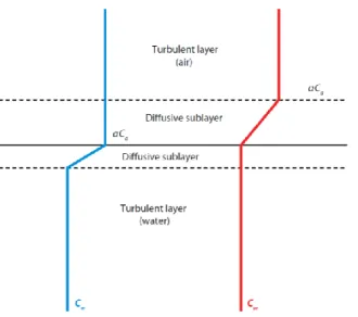
(1) Here, describes the grade of under- or oversaturation of the gas in the ocean and, thus, the direction of the flux and k determines the rate of exchange. The most commonly used simple conceptual model for air-sea exchange is the two layer model (Liss et al., 1974) (Figure 12). In the model, the turbulent atmospheric and oceanic boundary layers, where compounds are well-mixed and concentrations are homogeneous, are separated from the interface by two diffusive layers, one on each side of the interface. In the diffusive layers turbulence is suppressed and transport is realized only through molecular diffusion. This creates concentration gradients and imposes a resistance to the exchange from the air and from the water side, which can be parameterized.
The resistances depend on the solubility of the gas in water, which is described by Henry’s Law. The Henry’s Law constants (H) and their dependence on temperature were investigated by Moore and coworkers for halocarbons (Moore et al., 1995a; Moore et al., 1995b) and by De Bruyn et al. (1995) for DMS. For gases with low solubility, the air-side resistance is much higher than the water-side resistance, which results in the use of the transfer velocity in water and the concentrations of water and air in Eq. 1. There are several parameterizations available for the transfer velocity. Since the bulk air and water concentrations are measured in the turbulent layers, the transfer velocity correlates with wind speed, which determines the turbulence that drives the exchange. Additionally, the Schmidt Number (Sc) is used to describe the resistance of molecular diffusion in the water. Nightingale et al. (2000) developed a parameterization for the transfer velocity ( ) based on the wind speed at 10 m above the surface (u10) and a Schmidt number of 600 for CO2 at 20˚C in fresh water.
Figure 12: Two layer model of air-sea gas exchange from Liss et al. (1974), displayed in Wanninkhof et al. (2009). Abbreviations: concentration in water (cw), concentration in air (ca), Ostwald solubility coefficient (a).
(2) The wind speed at 10 m height (u10) is used for this parameterization. The Schmidt number has to be adapted for the different compounds. A compound-specific transfer coefficients is determined through an exponential relation like in Quack et al. (2003):
(3)
The spread between the different parameterizations of the transfer velocity is large, especially at high wind speeds. Nightingale et al. (2000) provide an estimate around the mean of known parameterizations (Lennartz et al., 2015). This bulk flux calculation method is a simplified approach to describe the more complicated real world and, thus, includes uncertainties through for example the negligence of effects of rain, bubbles, and surfactants.
1.2.3 VSLS emission estimates
Global estimates of VSLS emissions from the oceans vary strongly due to sparse observation data and the high spatial and temporal variability of emissions. Additionally the short lifetimes in the atmosphere make it difficult to accurately model emissions from atmospheric measurements. The first global emission estimates were made for CHBr3 and assumed homogeneous emissions (Penkett, WMO 1998, Dvortsov 1999, Carpenter and Liss 2000, Nielsen and Douglas 2001). Afterwards the geographical distribution of emissions was added and estimates were extrapolated from oceanic and atmospheric measurements, the so-called bottom-up approach (Quack et al., 2003; Smythe-Wright et al., 2005; Yokouchi et al., 2005; Butler et al., 2007). When atmospheric modeling became available and chemistry was included into the models, emissions were also inferred from observed atmospheric mixing ratios through a top-down approach (Warwick et al., 2006;
Kerkweg et al., 2008; Liang et al., 2010; Pyle et al., 2011). Ordóñez et al. (2012) coupled tropical emissions to chlorophyll a (Chl a) concentrations in the surface ocean and created an emission inventory that included seasonality. This is a rough approach, because the correlation with Chl a is mostly weak, since bromocarbon production appears more related to phytoplankton production, influenced by the phytoplankton species and the state of the bloom (Carpenter et al., 2009; Liu et al., 2011; Hepach et al., 2014;
Hepach et al., 2015). All other previously described emission inventories only report annual mean emissions. Ziska et al. (2013) created a CHBr3, CH2Br2, and CH3I emission
climatology from the HalOcAt database (https://halocat.geomar.de/) of limited oceanic and atmospheric halocarbon observations between 1989 and 2011 including seasonal and interannual variability through the physical parameters. Recently, halocarbon production in the ocean was modeled with ocean biogeochemical models to infer if models can reproduce observed emission patterns (Stemmler et al., 2013; Stemmler et al., 2015). The spread between the emission inventories is large and emissions in undersampled regions remain uncertain. It is hard to accurately model the stratospheric entrainment of halogenated VSLS from uncertain global estimates.
For DMS the data basis is better. Over the open ocean, DMS is hypothesized to be the most important precursor for non-sea salt sulfate aerosols, which influence climate through direct negative radiative forcing (Myhre et al., 2013) and serve as cloud condensation nuclei (Glasow et al., 2004). The formulation of a possible climate feedback mechanism, the CLAW-hypothesis, involving the DMS influence on clouds (Charlson et al., 1987) started a large number of field observations and modeling studies (e.g. Kloster et al., 2006; Marandino et al., 2013; Zindler et al., 2013), which led to an improved understanding of DMS sources to the atmosphere, although the feedback mechanism has not been verified yet. The result is a monthly resolved emission estimate for the global ocean (Lana et al., 2011). Nonetheless, there are many oceanic regions that are still undersampled and the IO is one notable example where the total emissions remain uncertain.
The observations of halogenated VSLS from the Indian Ocean are too sparse to be conclusive (Ziska et al., 2013), but single observations and modeling studies show a high potential for large emissions. High oceanic concentrations in the Arabian Sea and Bay of Bengal (Yamamoto et al., 2001; Roy et al., 2011), as well as modeling studies using atmospheric measurements (Liang et al., 2014), suggest high emissions for the Indian Ocean. For DMS, several observations exist from the Indian Ocean, but still far less than from other ocean basins (Lana et al., 2011). The predicted DMS emissions from the Indian Ocean are high. The Indian Ocean is a region with need for observations of VSLS in the atmosphere and water. The emissions from the Indian Ocean could be important for stratospheric ozone chemistry, if an efficient pathway from the boundary layer to the stratosphere through the Asian summer monsoon existed.
1.2.4 Atmospheric degradation and lifetimes
The atmospheric abundances of VSLS depend on oceanic emissions, transport processes and the degradation of these substances in the atmosphere. Their atmospheric mixing ratios are highly variable because of the short lifetimes and the spatial and temporal variation of emissions. Mixing ratios are high close to the emission sources and rapidly decrease with distance. A VSLS is defined as a substance with an atmospheric lifetime of less than half a year. The lifetime is defined as the time in which the amount of substance has degraded to 1/e.
The brominated VSLS CHBr3 and CH2Br2 degrade into soluble substances through reaction with the hydroxyl radical (OH) or photolysis (McGivern et al., 2002). For CHBr3
the main degradation reaction is photolysis and the main products are CBr2O and CHBrO.
These further react to HBr, HOBr, or BrO, which are summarized under Bry. CH2Br2 is mainly oxidized with OH or Cl radicals and also contribute to Bry. The Bry in the atmosphere can be washed out with rain (Hossaini et al., 2010). It can also react with ozone both in the troposphere or stratosphere or lead to particle formation (Yang et al., 2005; Saiz-Lopez et al., 2012). Atmospheric CH3I is photolyzed rapidly in the atmosphere into CH2I radicals and iodine atoms (Saiz-Lopez et al., 2012). Iodine reacts with ozone to iodine oxide (IO). I and IO together are called active iodine (IOx). They take part in the tropospheric ozone cycle (Vogt et al., 1999; Saiz-Lopez et al., 2012) and contribute to ozone depletion in the stratosphere (Solomon et al., 1994). Atmospheric active iodine can also form aerosols (O'Dowd et al., 2002) and ultrafine particles (Saiz- Lopez et al., 2012). Atmospheric DMS is degraded even faster than the halocarbons. It is mainly oxidized with OH into methyl sulfonic acid (MSA) or sulfur dioxide (SO2) (see e.g. Hoffmann et al., 2016, for more details). SO2 can create H2SO4, which condenses on existing particles or creates new ones, while MSA mainly condenses on existing particles adding to their mass but suppressing new particle formation.
Lifetime estimates of VSLS result from observations, laboratory experiments, and modeling the degradation processes in chemistry models. The lifetimes vary with height, latitude, and season and are therefore often modeled as lifetime profiles (Hossaini et al., 2010) (Figure 13). The most recent summary of lifetime estimates for halocarbons is given by Carpenter et al. (2014) and summarized in Table 1. The lifetime of DMS has been estimated from laboratory studies and observations (Barnes et al., 2006; Osthoff et al., 2009).
Figure 13: Annual tropical (±20˚) atmospheric lifetime profiles of (a) CHBr3 and (b) CH2Br2 calculated from a chemistry transport model (Hossaini et al., 2010).
Table 1: Tropical atmospheric lifetimes of VSLS at different altitudes for halogenated VSLS (Carpenter et al., 2014) and for DMS (Barnes et al., 2006; Osthoff et al., 2009).
1.2.5 VSLS entrainment to the stratosphere
After emission from the oceans, VSLS can be transported to stratosphere. Transport processes are important for the injection of oceanic VSLS to the stratosphere, because their lifetimes are comparable to transport timescales in the troposphere. Thus, the transport of VSLS to the stratosphere occurs primarily in the tropics and is connected with fast convection and ascent of air masses through the TTL (Figure 9).
Atmospheric lifetimes
Compound Boundary layer 10 km
CHBr3 15 d 17 d
CH2Br2 94 d 150 d
CH3I 4.0 d 3.5 d
DMS 11 min – 46 h 11 min – 46 h