Delivery of halogenated very short-lived substances from the west Indian Ocean to the stratosphere during the Asian summer monsoon

(1)

https://doi.org/10.5194/acp-17-6723-2017

Delivery of halogenated very short-lived substances from the west Indian Ocean to the stratosphere during the Asian summer monsoon

Alina Fiehn^1,2, Birgit Quack¹, Helmke Hepach^1,a, Steffen Fuhlbrügge¹, Susann Tegtmeier¹, Matthew Toohey¹, Elliot Atlas³, and Kirstin Krüger²

1GEOMAR Helmholtz Centre for Ocean Research Kiel, Kiel, Germany

2Meteorology and Oceanography Section, Department of Geosciences, University of Oslo, Oslo, Norway

3Rosenstiel School of Marine and Atmospheric Science, University of Miami, Miami, USA

anow at: Environment Department, University of York, York, UK Correspondence to:Kirstin Krüger (kkrueger@geo.uio.no) Received: 5 January 2017 – Discussion started: 11 January 2017

Revised: 21 April 2017 – Accepted: 2 May 2017 – Published: 8 June 2017

Abstract.Halogenated very short-lived substances (VSLSs) are naturally produced in the ocean and emitted to the atmosphere. When transported to the stratosphere, these compounds can have a significant influence on the ozone layer and climate. During a research cruise on RV Sonne in the subtropical and tropical west Indian Ocean in July and August 2014, we measured the VSLSs, methyl iodide (CH3I) and for the first time bromoform (CHBr3)and dibromomethane (CH2Br2), in surface seawater and the marine atmosphere to derive their emission strengths. Using the La- grangian particle dispersion model FLEXPART with ERA- Interim meteorological fields, we calculated the direct contribution of observed VSLS emissions to the stratospheric halogen burden during the Asian summer monsoon. Fur- thermore, we compare the in situ calculations with the interannual variability of transport from a larger area of the west Indian Ocean surface to the stratosphere for July 2000–

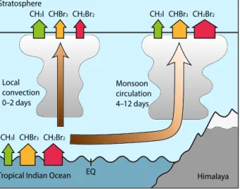
2015. We found that the west Indian Ocean is a strong source for CHBr₃ (910 pmol m⁻²h⁻¹), very strong source for CH2Br2(930 pmol m⁻²h⁻¹), and an average source for CH3I (460 pmol m⁻²h⁻¹). The atmospheric transport from the tropical west Indian Ocean surface to the stratosphere experiences two main pathways. On very short timescales, especially relevant for the shortest-lived compound CH₃I (3.5 days lifetime), convection above the Indian Ocean lifts oceanic air masses and VSLSs towards the tropopause. On a longer timescale, the Asian summer monsoon circulation transports oceanic VSLSs towards India and the Bay of Ben- gal, where they are lifted with the monsoon convection and

reach stratospheric levels in the southeastern part of the Asian monsoon anticyclone. This transport pathway is more important for the longer-lived brominated compounds (17 and 150 days lifetime for CHBr₃and CH₂Br₂). The entrainment of CHBr3 and CH3I from the west Indian Ocean to the stratosphere during the Asian summer monsoon is lower than from previous cruises in the tropical west Pacific Ocean during boreal autumn and early winter but higher than from the tropical Atlantic during boreal summer. In contrast, the projected CH₂Br₂entrainment was very high because of the high emissions during the west Indian Ocean cruise. The 16- year July time series shows highest interannual variability for the shortest-lived CH₃I and lowest for the longest-lived CH₂Br₂. During this time period, a small increase in VSLS entrainment from the west Indian Ocean through the Asian monsoon to the stratosphere is found. Overall, this study confirms that the subtropical and tropical west Indian Ocean is an important source region of halogenated VSLSs, especially CH₂Br₂, to the troposphere and stratosphere during the Asian summer monsoon.

1 Introduction

Natural halogenated volatile organic compounds in the ocean originate from chemical and biological sources like phytoplankton and macroalgae (Carpenter et al., 1999; Quack and Wallace, 2003; Moore and Zafiriou, 1994; Hughes et al., 2011). When emitted to the atmosphere, the halogenated very

(2)

short-lived substances (VSLSs) have atmospheric lifetimes of less than half a year (Law et al., 2006). Current estimates of tropical tropospheric lifetimes are 3.5, 17, and 150 days for methyl iodide (CH₃I), bromoform (CHBr₃), and dibromomethane (CH₂Br₂), respectively (Carpenter et al., 2014).

VSLSs can be transported to the stratosphere by tropical deep convection, where they contribute to the halogen burden, take part in ozone depletion, and thus impact the climate (Solomon et al., 1994; Dvortsov et al., 1999; Hossaini et al., 2015).

CHBr₃ is an important biogenic VSLS due to its large oceanic emissions and because it carries three bromine atoms per molecule into the atmosphere (Quack and Wallace, 2003;

Hossaini et al., 2012). CH2Br2 has a longer lifetime than CHBr3and thus a higher potential for stratospheric entrainment. CH3I is an important carrier of organic iodine from the ocean to the atmosphere and the most abundant organic iodine compound in the atmosphere (Manley et al., 1992;

Moore and Groszko, 1999; Yokouchi et al., 2008). Despite its very short atmospheric lifetime, it can deliver iodine to the stratosphere in tropical regions (Solomon et al., 1994;

Tegtmeier et al., 2013). Ship-based observations showed that bromocarbon emissions near coasts and in oceanic upwelling regions are generally higher than in the open ocean, because of macroalgal growth near coasts (Carpenter et al., 1999) and enhanced primary production in upwelling regions (Quack et al., 2007), while coastal anthropogenic sources also need to be considered (Quack and Wallace, 2003; Fuhlbrügge et al., 2016b). Measurements of VSLSs in the global oceans are sparse and the data show large variability. Thus, attempts at creating observation-based global emission estimates and cli- matologies (bottom-up approach; Quack and Wallace, 2003;

Butler et al., 2007; Palmer and Reason, 2009; Ziska et al., 2013), modeling the global distribution of halogenated VSLS emissions from atmospheric abundances (the top-down approach; Warwick et al., 2006; Liang et al., 2010; Ordóñez et al., 2012), and biogeochemical modeling of oceanic concentrations (Hense and Quack, 2009; Stemmler et al., 2013, 2015) are subject to large uncertainties (Carpenter et al., 2014). Global modeled top-down estimates (Warwick et al., 2006; Liang et al., 2010; Ordóñez et al., 2012) yield higher emissions than bottom-up estimates (Ziska et al., 2013;

Stemmler et al., 2013, 2015), which may indicate the im- portance of localized emission hot spots underrepresented in current bottom-up estimates.

The amount of oceanic bromine from VSLSs entrained into the stratosphere is estimated to be 2–8 ppt, which is 10–

40 % of the currently observed stratospheric bromine loading (Dorf et al., 2006; Carpenter et al., 2014). This wide range results mainly from uncertainties in tropospheric degrada- tion and removal, transport processes, and especially from the spatial and temporal emission variability of halogenated VSLS (Carpenter et al., 2014; Hossaini et al., 2016). Analyz- ing the time period 1993–2012, Hossaini et al. (2016) found no clear long-term transport-driven trend in the stratospheric

injection of oceanic bromine sources during a multi-model intercomparison.

Transport processes strongly impact stratospheric injec- tions of VSLSs, because their lifetimes are comparable to tropospheric transport timescales from the ocean to the stratosphere. The main entrance region of tropospheric air into the stratosphere is above the tropical west Pacific. Another active region lies above the Asian monsoon region during the boreal summer (Newell and Gould-Stewart, 1981), when the Asian monsoon circulation provides an efficient transport pathway from the atmospheric boundary layer to the lower stratosphere (Park et al., 2009; Randel et al., 2010).

Above India and the Bay of Bengal, convection lifts boundary layer air rapidly into the upper troposphere (Park et al., 2009; Lawrence and Lelieveld, 2010). As a response to the persistent deep convection, an anticyclone forms in the upper troposphere and lower stratosphere above Central, South, and East Asia (Hoskins and Rodwell, 1995). This so-called Asian monsoon anticyclone confines the air masses that have been lifted to this level within the anticyclonic circulation (Park et al., 2007; Randel et al., 2010). For the period 1951–

2015, a decreasing trend in rainfall and thus convection has been reported over northeastern India, which was caused by a weakening northward moisture transport over the Bay of Bengal (Latif et al., 2016).

Chemical transport studies in the Asian monsoon region have mostly focused on water vapor entrainment to the stratosphere (Gettelman et al., 2004; James et al., 2008) or on the transport of anthropogenic pollution (Park et al., 2009).

The chemical composition and source regions for air masses in the Asian monsoon anticyclone have been the topic of more recent studies (Bergman et al., 2013; Vogel et al., 2015;

Yan and Bian, 2015). Chen et al. (2012) investigated air mass boundary layer sources and stratospheric entrainment regions based on a climatological domain-filling Lagrangian study in the Asian summer monsoon area. The west Pacific Ocean and the Bay of Bengal are found to be important source regions, while maximum stratospheric entrainment occurred above the tropical west Indian Ocean.

The Asian monsoon circulation could be an important pathway for the stratospheric entrainment of oceanic VSLSs (Hossaini et al., 2016), because the steady southwest monsoon winds in the lower troposphere during boreal summer deliver oceanic air masses from the tropical Indian Ocean towards India and the Bay of Bengal (Lawrence and Lelieveld, 2010), where they are lifted by the monsoon convection and the Asian monsoon anticyclone. However, little is known about the emission strength of VSLSs from the Indian Ocean and their transport pathways. A few measurements in the Bay of Bengal (Yamamoto et al., 2001) and Arabian Sea (Roy et al., 2011) as well as global source estimates suggest that the Indian Ocean might be a considerable source (Liang et al., 2010; Ziska et al., 2013). No bromocarbon data are available for the equatorial and southern Indian Ocean, yet, but CH₃I, which has been measured around the Mascarene Plateau,

(3)

showed high oceanic concentrations (Smythe-Wright et al., 2005). Liang et al. (2014) use a chemistry climate model for the years 1960 to 2010 and modeled that the tropical In- dian Ocean delivers more bromine to the stratosphere than the tropical Pacific because of its higher atmospheric surface concentrations based on the global top-down emission estimate by Liang et al. (2010).

In this study, we show surface ocean concentrations and atmospheric mixing ratios of the halogenated VSLS CH₃I, and for the first time for CHBr₃and CH₂Br₂, in the subtropical and tropical west Indian Ocean during the Asian summer monsoon. We use the Lagrangian particle dispersion model FLEXPART to investigate the atmospheric transport pathways of observation-based oceanic VSLS emissions to the stratosphere.

Our questions for this study are as follow: is the tropical Indian Ocean a source for atmospheric VSLS? What is the transport pathway from the west Indian Ocean to the stratosphere during the Asian summer monsoon? How many VSLSs are delivered from the west Indian Ocean to the stratosphere during the Asian summer monsoon? How large is the interannual variability of this VSLS entrainment?

In Sect. 2, we describe the cruise data and the transport model simulations. In Sect. 3, the results from the cruise measurements and trajectory calculations are shown and discussed. Then, the spatial and interannual variability of transport is presented in Sect. 4. In Sect. 5, we address uncertainties before summarizing the results and concluding in Sect. 6.

2 Data and methods

2.1 Observations during the cruise

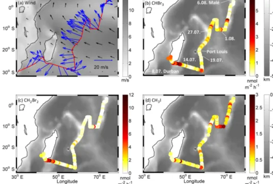
During two consecutive research cruises in the west Indian Ocean, we observed meteorological, oceanographic, and biogeochemical conditions, including atmospheric mixing ratios and oceanic concentrations of halogenated VSLSs. The two cruises on RVSonne, SO234-2 from 8 to 19 July 2014 (Durban, South Africa to Port Louis, Mauritius) and SO235 from 23 July to 7 August 2014 (Port Louis, Mauritius to Malé, Maldives), were conducted within the SPACES (Sci- ence Partnerships for the Assessment of Complex Earth Sys- tem Processes) and OASIS (Organic very short-lived Sub- stances and their air sea exchange from the Indian Ocean to the Stratosphere) research projects. Cruise SO234-2 was an international training and capacity building program for students from Germany and southern African countries, whereas SO235 was purely scientifically oriented. The cruise tracks covered subtropical waters, coastal and shelf areas, and the tropical open west Indian Ocean and were designed to cover biologically productive and nonproductive regions (Fig. 1). In the following, we will refer to the combined cruises as the “OASIS cruise”.

We collected meteorological data from ship-based sensors including surface air temperature (SAT), relative humidity, air pressure, wind speed and direction taken every second at about 25 m height on RVSonne. Sea surface temperature (SST) and salinity were measured in the ship’s hydrographic shaft at 5 m depth. We averaged all parameters to 10 min in- tervals for our investigations.

During the cruise, we launched 95 radiosondes and thus obtained high-resolution atmospheric profiles of temperature, wind, and humidity. During the first half of the cruise, regular radiosondes were launched at 00:00 and 12:00 UTC and additionally at 06:00 and 18:00 UTC during the 48 h sta- tion (16–18 June 2014; Fig. 1). During the second half of the cruise, the launches were always performed at standard UTC times (00:00, 06:00, 12:00, 18:00 UTC) and every 3 h during the diurnal stations (26 and 28 June, 3 August 2014).

For the regular launches, we used GRAW DFM-09 radiosondes, and for the six ozonesonde launches we used DFM- 97. The collected radiosonde data was delivered in near real time to the Global Telecommunication System (GTS) to im- prove meteorological reanalyses (e.g., European Centre for Medium-Range Weather Forecasts, ECMWF, Re-Analysis Interim, ERA-Interim) and operational forecast models (e.g., opECMWF, operational ECMWF) in the subtropical and tropical west Indian Ocean.

Trace gas emissions are generally well mixed within the marine atmospheric boundary layer (MABL) on timescales of an hour or less by convection and turbulence (Stull, 1988).

We determined the stable layer that defines the top of the MABL with the practical approach described in Seibert et al. (2000). From the radiosonde ascent we computed the vertical gradient of virtual potential temperature, which indicates the stable layer at the top of the MABL with positive values. A detailed description of our method can be found in Fuhlbrügge et al. (2013).

We collected a total of 213 air samples with a 3-hourly resolution at about 20 m height above sea level. These samples were pressurized to 2 atm in pre-cleaned stainless steel can- isters with a metal bellows pump, and they were analyzed within 6 months after the cruise. Details about the analysis, the instrumental precision, the preparation of the samples, and the use of standard gases are described in Schauf- fler et al. (1999), Montzka et al. (2003), and Fuhlbrügge et al (2013).

We collected overall 154 water samples, spaced about every 3 h, from the hydrographic shaft of RVSonneat a depth of 5 m. The samples were then analyzed for halogenated compounds using a purge and trap system onboard, which was attached to a gas chromatograph with an electron cap- ture detector. An analytical reproducibility of 10 % was determined from measuring duplicate water samples. Calibra- tion was performed with a liquid mixed-compound standard prepared in methanol. Details of the procedure can be found in Hepach et al. (2016).

(4)

Figure 1. (a)July 2014 average wind speed (gray shading) and direction (black) from ERA-Interim and 10 min mean wind speed (blue arrows) from ship sensors;(b)CHBr₃,(c)CH₂Br₂, and(d)CH₃I emissions derived from OASIS cruise on July–August 2014 and bathymetry.

The sea–air flux (F )of the VSLSs was calculated from the transfer coefficient (k_w)and the concentration gradient (1c)according to Eq. (1). The gradient is between the water concentration (c_w)and the theoretical equilibrium water concentration (c_atm/H ), which is derived from the atmospheric concentration (catm). We use Henry’s law constants (H )of Moore and coworkers (Moore et al., 1995a, b).

F =k_w·1c=k_w ·

c_w−catm

H

(1) Compound-specific transfer coefficients were determined using the air–sea gas exchange parameterization of Nightingale et al. (2000) and by applying a Schmidt number (Sc) for the different compounds as in Quack and Wallace (2003) (Eq. 2).

kw=k· Sc⁻¹²

600 (2)

Nightingale et al. (2000) determined the transfer coefficient (k) as a function of the wind speed at 10 m height (u₁₀):

k=2u²₁₀+3u₁₀. This wind speed is derived from a logarith- mic wind profile using the von Kármán constant (κ=0.41), the neutral drag coefficient (Cd)from Garratt (1977), and the 10 min average of the wind speed (u(z)) measured at z=25 m during the cruise (Eq. 3):

u10=u (z) κ√ C_d κ√

C_d+log₁₀^z . (3)

2.2 Trajectory calculations

For our trajectory calculations, we use the Lagrangian particle dispersion model FLEXPART of the Norwegian Insti- tute for Air Research in the Atmosphere and Climate De- partment (Stohl et al., 2005), which has been evaluated in previous studies (Stohl et al., 1998; Stohl and Trickl, 1999).

The model includes moist convection and turbulence parameterizations in the atmospheric boundary layer and free troposphere (Stohl and Thomson, 1999; Forster et al., 2007).

In this study, we employ the most recently released version 9.2 of FLEXPART, modified to incorporate lifetime profiles.

We use the ECMWF reanalysis product ERA-Interim (Dee et al., 2011) with a horizontal resolution of 1^◦×1^◦ and 60 vertical model levels as meteorological input fields, provid- ing air temperature, winds, boundary layer height, specific humidity, and convective and large scale precipitation with a 6-hourly temporal resolution. The vertical winds in hybrid coordinates were calculated mass-consistently from spectral data by the pre-processor (Stohl et al., 2005). We record the transport model output every 6 h.

We ran the FLEXPART model with three different setups, which are described in Table 1. These configurations are des- ignated as (1) OASIS back (backward trajectories), (2) OA- SIS (forward trajectories), and (3) Indian Ocean (regional forward trajectories).

We calculated OASIS backward trajectories from the 12:00 UTC locations of RVSonneduring the cruise. These trajectories are later used to determine the source regions of air masses investigated along the cruise track.

(5)

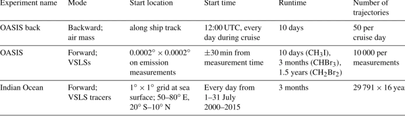
Table 1.FLEXPART experimental setups including experiment name, mode, start location and time, runtime, and number of trajectories.

Experiment name Mode Start location Start time Runtime Number of

trajectories OASIS back Backward;

air mass

along ship track 12:00 UTC, every day during cruise

10 days 50 per

cruise day

OASIS Forward;

VSLSs

0.0002^◦×0.0002^◦ on emission measurements

±30 min from measurement time

10 days (CH₃I), 3 months (CHBr₃), 1.5 years (CH₂Br₂)

10 000 per measurements Indian Ocean Forward;

VSLS tracers

1^◦×1^◦grid at sea surface; 50–80^◦E, 20^◦S–10^◦N

Every day from 1–31 July 2000–2015

3 months 29 791×16 years

With the OASIS setup, we study the transport of oceanic CHBr₃, CH₂Br₂, and CH₃I emissions from the measurement locations into the stratosphere similar to what was carried out in the corresponding study by Tegtmeier et al. (2012).

At every position along the cruise track at which emissions were calculated (Sect. 2.1), we release a mass of the compound equal to a release from 0.0002^◦×0.0002^◦in 1 h. The mass is evenly distributed among 10 000 trajectories. During transport, CHBr₃ and CH₂Br₂ mass is depleted according to atmospheric lifetime profiles from Hossaini et al. (2010) based on chemistry transport model simulations including VSLS chemistry. CH₃I decays by applying a uniform vertical lifetime of 3.5 days (Sect. 1). The mass on all trajectories that reaches a height of 17 km is summed and assumed to be entrained into the stratosphere. This threshold height represents the average cold point tropopause (CPT) height during the cruise (see Fig. S1 in the Supplement) and also for the whole tropics (Munchak and Pan, 2014). The influence of the entrainment height criteria is further discussed in Sect. 4. For intercomparison with other ocean basins, we employed exactly the same model setup of transport simulations (including lifetimes) and the same emission calculation method for three previous corresponding cruises in the tropics: the TransBrom campaign in the west Pacific in 2009 (introduction to special issue: Krüger and Quack, 2013), the SHIVA campaign in the South China and Sulu seas in 2011 (Fuhlbrügge et al., 2016a), and the MSM18/3 cruise in the equatorial Atlantic cold tongue (Hepach et al., 2015).

The transport calculations based on the measured emissions from OASIS give insight into the contribution of oceanic emissions to the stratosphere during the Asian summer monsoon. However, transport and emissions in the OA- SIS study are localized in space and time and could thus be very different for different areas and years. In order to investigate the transport from the west Indian Ocean basin to the stratosphere and its interannual variability under the influence of the Asian summer monsoon circulation (Indian Ocean setup), we calculate trajectories from a large region of the tropical west Indian Ocean surface for the years 2000–

2015. Trajectories are uniformly started within the release

area (50–80^◦E, 20^◦S–10^◦N), covering the tropical west In- dian Ocean, once every day during the month of July in 2000–2015. The run time is set to 3 months, which covers the period from July to October. We then calculate the frac- tion (q)of each VSLS tracer that reaches the stratosphere during the transit time (t t), assuming an exponential decay of the tracer (Eq. 4) according to the tropical tropospheric lifetimes (lt) of 17, 150, and 3.5 days for CHBr₃, CH₂Br₂, and CH₃I, respectively (Carpenter et al., 2014).

q=e⁻^{t t}^lt (4)

We use the term “VSLS tracer” to distinguish from the calculations used in the OASIS setup, where actual VSLS emissions experience decay according to a vertical lifetime profile (uniform for CH3I). The use of VSLS tracers allows us to evaluate one model run for different compounds with varying lifetimes. This Indian Ocean setup provides information on the preferred pathways from the west Indian Ocean to the stratosphere for different transport timescales and on their interannual variability. This variability is quantified by the coefficient of variation (CV), which is defined as the ratio of the standard deviation to the mean entrainment. The correlations of the interannual variations between different regions of stratospheric entrainment are given by the correlation coefficient (r)by Pearson (1895). We calculated thepvalue to determine the 95 % significance level of the correlations.

3 The Indian Ocean cruise: OASIS 3.1 Atmospheric circulation

SST and SAT during the OASIS cruise generally increase from the south towards the equator (Fig. 2a). The SST is on average 1.5^◦C higher than the SAT, which benefits convection. Minimum SSTs of 18^◦C were measured from 14 to 17 July 2014 in the open subtropical Indian Ocean (30^◦S, 59^◦E), and maximum SSTs of 29^◦C were measured around the equator.

(6)

Figure 2. (a)Surface air temperature (SAT), sea surface temperature (SST), and(b)wind speed and direction measured by ship sensors during the OASIS cruise in the Indian Ocean.(c)Water concentration;(d)atmospheric mixing ratio; and(e)emission of CHBr₃, CH₂Br₂, and CH₃I. The gray line denotes the harbor stop at Port Louis, Mauritius, 20–23 July 2014. Also note the nonlinear leftyaxes in(c)and(e).

The overall mean wind speed was 8.1 m s⁻¹, with lower wind speeds in the subtropics and close to the equator (5 m s⁻¹) and higher wind speeds (up to 15 m s⁻¹) in the trade wind region (23 July to 5 August, 20–5^◦S; Fig. 2b).

The mean wind direction during the cruise was southeast.

While the wind direction showed large variability in the subtropics, southeasterly trade winds dominated between Mau- ritius and the equator. North of the equator the wind direction changed to westerly winds. Our in situ ship wind measurements deviate from the mean July wind field from ERA- Interim during the first part of the cruise south of Mauritius (Fig. 1a) due to the influence of a developing low-pressure system (not shown). The steady trade winds during the second part of the cruise are well reflected in the July mean wind field from ERA-Interim. Surface winds from in situ ship measurements, radiosondes, and time-varying ERA-Interim data show good agreement (Fig. S2).

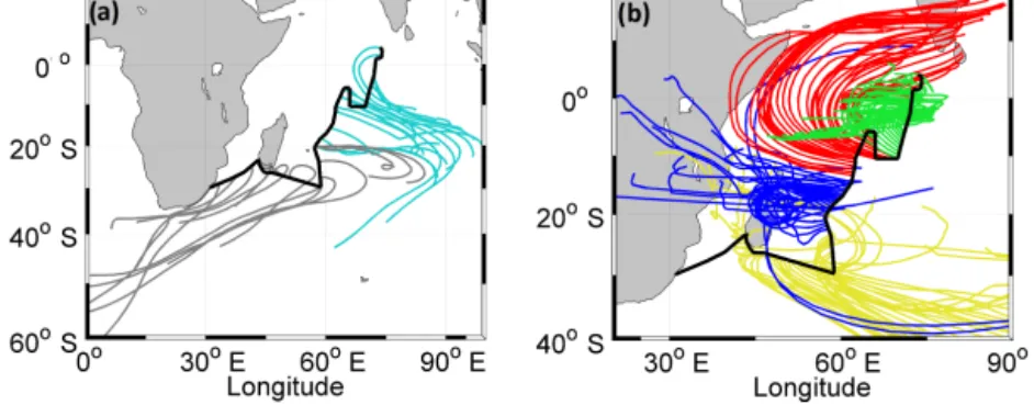
Air masses sampled during the cruise originate mainly from the open ocean (Fig. 3a). Trajectories started between South Africa and Mauritius generally come from the south.

An influence of terrestrial sources is possible close to South Africa and Madagascar. From Mauritius to the Maldives, the trajectories originate from the southeast open Indian Ocean.

The analysis of air samples reveal no recent fresh anthropogenic input, indicated by the very low levels of short- lived trace gas contaminants, e.g., butane (lifetime 2.5 days;

Finlayson-Pitts and Pitts, 2000), in this region (not shown).

3.2 VSLS observations and oceanic emissions

CHBr3, CH2Br2, and CH3I surface ocean concentrations, atmospheric mixing ratios, and emissions for the OASIS cruise are plotted as time series in Fig. 2c–e and are summarized in Table 2.

(7)

Figure 3. (a) FLEXPART 5-day backward trajectories for OASIS backward setup, averaged forn=50 trajectories, starting from ship positions daily at 12:00 UTC between 8 July and 7 August 2014. The Southern Ocean (gray) and the open Indian Ocean (turquoise) are source regions for air measured during the cruise.(b) FLEXPART 10-day forward trajectories for OASIS setup, averaged forn=1000 trajectories, starting at the ship positions of simultaneous VSLS measurements. Trajectories are colored according to their transport regimes:

Westerlies (yellow), Transition (blue), Monsoon Circulation (red), and Local Convection (green).

Table 2. CHBr₃, CH₂Br₂, and CH₃I water concentrations, atmospheric mixing ratios, and calculated emissions for the OASIS In- dian Ocean cruise. The table lists the average value of all measurements and 1 SD. The brackets give the range of measurements.

VSLS Water concentration (pmol L⁻¹)

Air mixing ratio (ppt)

Emission (pmol m⁻²h⁻¹)

CHBr₃ 8.4±14.2 [1.3–33.4]

1.20±0.35 [0.68–2.97]

910±1160 [−100–9630]

CH₂Br₂ 6.7±12.6 [0.6–114.3]

0.91±0.08 [0.77–1.20]

930±2000 [−70–19 960]

CH₃I 3.4±3.1 [0.2–16.4]

0.84±0.12 [0.57–1.22]

460±430 [5–2090]

CHBr₃ concentrations in the surface ocean range from 1.3 to 33.4 pmol L⁻¹, with an average of all measurements of 8.4±14.2 (1σ )pmol L⁻¹. The standard deviation (σ ) is used as a measure of the variability in the measurements during the cruise. We measured large water concentrations of > 10 pmol L⁻¹ close to coasts and shelf regions and in the open Indian Ocean between 5 and 10^◦S (27 July–2 Au- gust). Oceanic concentrations of CH2Br2are smaller, with a mean of 6.7±12.6 pmol L⁻¹, but show a similar distribution to CHBr3 concentrations. High concentrations were measured southeast of Madagascar, when we passed the southern stretch of the East Madagascar Current. Oceanic upwelling occurs along the eddy-rich, shallow region south of Madagascar, which leads to locally enhanced phytoplankton growth (Quartly et al., 2006). It is possible that an upwelling of elevated CH₂Br₂concentrations from the deeper ocean could have occurred in a similar way as was observed for the equatorial upwelling in the Atlantic (Hepach et al., 2015). CH₃I oceanic concentrations range from 0.2 to 16.4 pmol L⁻¹, with a mean of 3.4±3.1 pmol L⁻¹. They were elevated (5–12 pmol L⁻¹)during the last part of the

cruise (August 3–6, 2014) around the equator. In the region of the Mascarene Plateau, to the west of our cruise, Smythe- Wright et al. (2005) detected much larger CH₃I concentrations between 20 and 40 pmol L⁻¹during June–July 2002.

Atmospheric mixing ratios of CHBr3 during the OA- SIS cruise (Fig. 2d, Table 2) show an overall mean of 1.20±0.35 ppt. Elevated mixing ratios of > 2 ppt are found in three locations: south of Madagascar, in Port Louis, and close to the British Indian Ocean Territory. The first two probably have terrestrial or coastal sources, because they do not coin- cide with high oceanic CHBr₃concentrations, but backward trajectories pass land. Close to the British Indian Ocean Ter- ritory, oceanic concentrations and atmospheric mixing ratios are elevated, which suggests a local oceanic source. Atmo- spheric mixing ratios of CH₂Br₂ vary little around the average of 0.91 ppt and show a similar pattern to the CHBr₃ mixing ratios. CH₃I (0.84±0.12 ppt) mixing ratios reveal pronounced variations and surpass 1 ppt in some locations.

These atmospheric mixing ratios above the open ocean are much lower than the average of 12 pptv Smythe-Wright et al. (2005) reported around the Mascarene Plateau.

We calculated oceanic emissions from the synchronized measurements of surface water concentration and atmospheric mixing ratio as described in Sect. 2.1 (Figs. 2e and 1). Strong emissions are caused by high oceanic concentrations, high wind speeds, or a combination of both.

The OASIS emission strength of CHBr₃ ranges from

−100 to 9630 pmol m⁻²h⁻¹, with high mean emissions of 910±1160 pmol m⁻²h⁻¹; this is caused by moderate water concentrations and relatively high wind speeds. We derive the strongest emissions south of Madagascar and in the trade wind regime from 5 to 10^◦S above the open ocean upwelling region of the Seychelles-Chagos-thermocline ridge (Schott et al., 2009), where we also observed enhanced phytoplankton growth (not shown here). CH2Br2emissions (with an overall mean of 930±2000 pmol m⁻²h⁻¹)were by

(8)

far strongest south of Madagascar, with a single maximum of up to 20 000 pmol m⁻²h⁻¹. Here, we experienced very high oceanic concentrations and high wind speeds due to the pas- sage of a low-pressure system south of the ship track during 11–17 July 2014. CH₃I emissions (460±430 pmol m⁻²h⁻¹) had a pronounced maximum of 2090 pmol m⁻²h⁻¹around 10^◦S and 70^◦E (31 July–1 August), in accordance with high wind speeds and oceanic concentrations being elevated close to the above-mentioned open ocean upwelling observed between 5 and 10^◦S.

During the first part of the cruise, we recorded low mean atmospheric mixing ratios of CHBr3 and CH2Br2, despite high local oceanic concentrations and emissions especially south of Madagascar. In connection with a high and well- ventilated MABL (Fig. S1), this indicates that the strong sources south of Madagascar are highly localized. The oc- casional enhancement of the brominated VSLSs in some air samples underlines the patchiness of the sources in this region. During the second part of the cruise, the atmospheric mixing ratios of CHBr₃ and CH₂Br₂ increased from south to north and in the direction of the wind maximizing close to the equator (Fig. 2d). The emissions were strong between Mauritius and the equator (Fig. 2e). This suggests that the air around the equator was enriched by the advection of the oceanic emissions with the trade winds from south to north.

We assume that the bromocarbons accumulate because of the steady wind directions and the suppression of mixing into the free troposphere due to the top of the MABL and the trade inversion layer (Fig. S1, 27 July–2 August) acting as transport barriers for VSLSs as was observed for the Peruvian upwelling (Fuhlbrügge et al., 2016a).

3.3 Comparison of OASIS VSLS emissions with other oceanic regions

Average emissions of the three VSLSs from OASIS and other tropical cruises and modeling studies are summarized in Ta- ble 3. We compare with cruises and open ocean estimates, since OASIS mainly covered open ocean regions and only small coastal areas close to Madagascar, the British Indian Ocean Territory, and the Maldives.

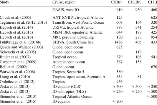
The average CHBr3emission during the OASIS campaign (910 pmol m⁻²h⁻¹)was larger than during most campaigns in tropical regions: 1.5 times larger than during TransBrom in the subtropical and tropical west Pacific (Tegtmeier et al., 2012), 1.2 times larger than during DRIVE in the tropical northeast Atlantic (Hepach et al., 2014), and 1.5 times larger than during MSM18/3 in the Atlantic equatorial upwelling (Hepach et al., 2015). Only the SHIVA campaign in the South China and Sulu seas yielded larger CHBr₃emissions of 1486 pmol m⁻²h⁻¹because of very high oceanic concentrations close to the coast (Fuhlbrügge et al., 2016b). The global open ocean estimate by Quack and Wallace (2003) is one-third smaller than our measured values in the west In- dian Ocean. The bottom-up emission climatology by Ziska

et al. (2013) estimates smaller values for the Indian Ocean, based on measurements from other oceanic basins due to a lack of available Indian Ocean in situ measurements. With their top-down approach, Warwick et al. (2006), Liang et al. (2010), and Ordóñez et al. (2012) derived CHBr₃ emissions in the range of 580–956 pmol m⁻²h⁻¹ for the tropical ocean. Stemmler et al. (2014) modeled very low CHBr₃ emissions around 200 pmol m⁻²h⁻¹for the equatorial Indian Ocean with their biogeochemical ocean model.

Average CH₂Br₂ emissions from the OASIS cruise (930 pmol m⁻²h⁻¹) are 2–6 times larger than the average cruise emissions listed in Table 3: TransBrom, DRIVE, MSM18/3, SHIVA, and M91. This is caused by the generally high oceanic concentrations during OASIS, with the largest values south of Madagascar. The mean emissions from the west Indian Ocean are also much stronger than the tropical ocean estimates from Butler et al. (2007) and the global open ocean estimate from Yokouchi et al. (2008) and Carpenter et al. (2009). The top-down model approach by Liang et al. (2010) yielded the weakest emissions at only 81 pmol m⁻²h⁻¹. The Ziska et al. (2013) climatology shows maximum equatorial Indian Ocean CH₂Br₂emission values of around 500 pmol m⁻²h⁻¹.

The average CH₃I emissions during OASIS (460 pmol m⁻²h⁻¹) were in the range of previously observed and estimated values from 254 to 625 pmol m⁻²h⁻¹ (Table 3). For the highly productive Peruvian upwelling, Hepach et al. (2016) calculated much larger emissions of 954 pmol m⁻²h⁻¹. The coupled ocean–atmosphere model of Bell et al. (2002) produced average global emissions of 670 pmol m⁻²h⁻¹, while Stemmler et al. (2013) modeled CH₃I emissions of around 500 pmol m⁻²h⁻¹for the tropical Atlantic with their biogeochemical ocean model. The Ziska et al. (2013) climatology shows Indian Ocean CH₃I emissions of around 500 pmol m⁻²h⁻¹.

In general, the emissions during the OASIS cruise in the subtropical and tropical west Indian Ocean were as strong as or stronger than in other tropical open ocean cruises or studies. CH₂Br₂ emissions during the OASIS cruise were especially stronger than any previous emissions estimates.

The west Indian Ocean seems to be a region with significant contribution to the global open ocean VSLS emissions, especially in the boreal summer when wind speeds are high because of the southwest monsoon circulation.

3.4 VSLS entrainment to the stratosphere during OASIS

The OASIS forward trajectories released at the locations of the VSLS measurements show the transport pathway of the air masses from their sample points along the cruise track (Fig. 3b). The mean of all 10 000 trajectories from each release can be grouped into four regimes according to transport direction: Westerlies, Transition, Monsoon Circulation, and Local Convection. The air masses in the Westerlies regime

(9)

Table 3.CHBr₃, CH₂Br₂, and CH₃I mean emissions (pmol m⁻²h⁻¹) for several cruises and observational and model-based climatological studies. Abbreviations: IO, Indian Ocean; OLS, ordinary least squares method.

Study Cruise, region CHBr₃ CH₂Br₂ CH₃I

OASIS, west IO 910 930 460

Chuck et al. (2005) ANT XVIII/1, tropical Atlantic 125 625

Tegtmeier et al. (2012, 2013) TransBrom, west Pacific Ocean 608 164 320

Hepach et al. (2014) DRIVE, tropical Atlantic 787 341 254

Hepach et al. (2015) MSM 18/3, equatorial Atlantic 644 187 425

Hepach et al. (2016) M91, peruvian upwelling 130 273 954

Fuhlbrügge et al. (2016b) SHIVA, South China Sea 1486 405 433 Quack and Wallace (2003) Global open ocean 625

Yokouchi et al. (2005) Global open ocean 119

Butler et al. (2007) Tropical ocean 379 108 541

Carpenter et al. (2009) Atlantic open ocean 367 158

Bell et al. (2002) Global ocean 670

Warwick et al. (2006) Tropics, Scenario 5 580

Liang et al. (2010) Tropics, open ocean, Scenario A 854 81

Ordoñez et al. (2012) Tropics 956

Ziska et al. (2013) IO equator (OLS) ≈500 ≈500 ≈250

Ziska et al. (2013) IO subtropics (OLS) ≈250 ≈250 ≈500

Stemmler et al. (2013) Tropical Atlantic Ocean ≈500

Stemmler et al. (2015) IO equator ≈200

are transported to the southeast Indian Ocean, and the air masses from the Transition regime propagate towards Mada- gascar and Africa. FLEXPART calculations reveal that both transport regimes lift air masses up to a mean height of about 5.3 km after 1 month (not shown here). The trajectories of the Monsoon Circulation regime first travel with the southeasterly trade winds and then with the southwesterly monsoon winds. The trajectories stay relatively close to the ocean surface (below 3 km) until they reach the Bay of Bengal, where they are rapidly lifted to the upper troposphere. On average they reach a height of 7.9 km after 1 month, which reveals that this is the regime with the most convection. The trajectories of the Local Convection regime mainly experience rapid uplift around the equator. After 1 month this group has reached a mean height of 7.2 km. The different uplifts are reflected in the vertical distribution of bromoform in each transport regime (Fig. S3).

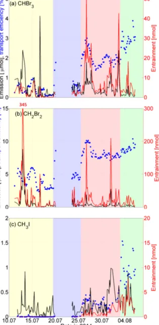
The absolute entrainment of oceanic VSLSs to the stratosphere depends on the emission strength as well as the transport efficiency (Fig. 4). This efficiency is defined as the ratio between entrained and emitted VSLSs. It depends on the transit time, defined as the time an air parcel needs to be transported from the ocean surface to 17 km height, and the lifetime of the compound. For stratospheric entrainment the transit time must be on the order of the lifetime of a compound or shorter. If the transit time is considerably larger than the lifetime, most of the compound decays before reaching the stratosphere. In the following, we will use the expressions VSLSs’ transit time, which is the transit time including loss processes of the VSLS in the atmosphere during the trans-

port, and transit half-life, which is the time after which half of the total amount of entrained tracer has been entrained above 17 km. We also calculated the relative emission and entrainment by regime. Table 4 displays the absolute and relative emissions and entrainment, the transport efficiency, and the transit half-life for the whole cruise and the four regimes.

The mean sea surface release of CHBr3 in FLEXPART is 0.43 µmol (on 0.0002^◦×0.0002^◦h⁻¹)during the cruise, and the mean entrainment to the stratosphere is 5.5 nmol, resulting in a mean transport efficiency of 1.3 %. CH₂Br₂ has a higher transport efficiency of 5.5 %, with mean emissions of 0.43 µmol (on 0.0002^◦×0.0002^◦h⁻¹)and very high stratospheric entrainment of 23.6 nmol. CH₃I has a low transport efficiency of 0.3 %, with mean emissions of 0.22 µmol (on 0.0002^◦×0.0002^◦ h⁻¹) and stratospheric entrainment of 0.7 nmol.

The four transport regimes show different transport efficiencies for CHBr₃, CH₂Br₂, and CH₃I to the stratosphere.

The two most efficient regimes, transporting CHBr3 and CH3I to the stratosphere during the OASIS cruise, were the Monsoon Circulation and the Local Convection regime.

The transport efficiency for all three compounds is highest in the Local Convection regime (CHBr3∼3 %, CH2Br2

∼9 %, and CH₃I∼1 %), because this regime has the shortest transit half-life for all three VSLSs. For CH₃I, the compound with the shortest lifetime, the fast transport plays the largest role, and thus this regime is by far the most efficient.

For CHBr₃, the regime with most absolute and relative stratospheric entrainment (11 nmol, 57 %) is the Monsoon Circulation regime because of the high emissions in the

(10)

Figure 4. CHBr₃, CH₂Br_2, and CH₃I emission entrainment at 17 km and transport efficiency for measurements from the OASIS cruise. The background shading highlights the transport regimes:

Westerlies (yellow), Transition (blue), Monsoon Circulation (red), and Local Convection (green).

source region and the high transport efficiency. Although the CHBr3 emissions are as high in the Westerlies regime, the entrainment is small (2 nmol, 9 %) because of a low transport efficiency due to slow transport visible in the long transit half-life. The Local Convection regime has the highest transport efficiency, but emissions were low, resulting in less entrainment (4 nmol, 23 %) than in the Monsoon Circula- tion regime. The absolute entrainment of CH₂Br₂ strongly depends on the strength of emission, because the transport efficiency is relatively similar for all transport regimes due to the long lifetime of the compound. Most entrained CH₂Br₂comes from the Westerlies regime (29 nmol, 35 %),

where sources especially south of Madagascar were ex- tremely strong. Although these emissions occur in the subtropics, they reach 17 km mainly in the tropics (Fig. S4).

The transport efficiency of 4 % still allows a large amount of 345 nmol CH₂Br₂to enter the stratosphere from the maximum emissions at 23:00 UTC on 12 July 2014 (Fig. 4). The CH₃I absolute entrainment (2.8 nmol, 79 %) is highest in the Local Convection regime because of both the highest emissions and highest transport efficiency (Table 4).

3.5 Comparison of VSLS entrainment to the stratosphere with other oceanic regions

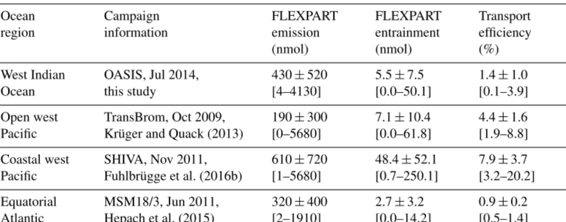
A comparison of the subtropical and tropical Indian Ocean contribution to the stratosphere with other tropical ocean regions, applying the same emission calculation and model setup (Sect. 2.2) for CHBr₃, is shown in Table 5. Though the western Pacific TransBrom cruise had lower bromoform emission rates compared to OASIS, stratospheric entrainment was greater for the western Pacific region compared to the Indian Ocean. This difference was caused by a higher transport efficiency of 4.4 % in the west Pacific influenced by tropical cyclone activity in October 2009 (Krüger and Quack, 2013). Tegtmeier et al. (2012) obtained a higher transport efficiency of 5 % for TransBrom using a previous FLEX- PART model (version 8.0). During the SHIVA campaign in the South China Sea, high oceanic concentrations of bromoform produced mean emission rates that were higher than during OASIS. The SHIVA calculations show even higher transport efficiencies of 7.9 %, which lead to an entrainment of 48.4 nmol CHBr3 (Table 5), because of the strong convective activity in that region during the time (Fuhlbrügge et al., 2016b). The MSM18/3 cruise in the equatorial Atlantic (Hepach et al., 2015) has the smallest emissions, entrainment, and a transport efficiency of 0.9 % (Table 5). Overall, the comparison indicates that more CHBr₃was entrained to the stratosphere from the tropical west Pacific than from the tropical west Indian Ocean during the Asian summer monsoon using available in situ emissions and 6-hourly meteorological fields. This is in contrast to the study by Liang et al. (2014), who determined with a chemistry climate model climatology that emissions from the tropical Indian Ocean deliver more brominated VSLSs into the stratosphere than tropical west Pacific emissions.

CH2Br2entrainment to the stratosphere for the TransBrom ship campaign was∼8 nmol with transport efficiencies of 15 % (Tegtmeier et al., 2012). This is much higher than the Indian Ocean transport efficiency of 6.4 %, but the absolute entrainment of 23.6 nmol CH₂Br₂we calculated for the OA- SIS cruise (Table 4) is much higher than during TransBrom, because of the very strong CH₂Br₂emissions during OASIS.

Tegtmeier et al. (2013) investigated CH₃I entrainment to the stratosphere for three tropical ship campaigns: SHIVA and TransBrom in the tropical west Pacific and DRIVE in the tropical northeast Atlantic. They used a CH₃I lifetime

(11)

Table 4.Mean FLEXPART emission, entrainment at 17 km, transport efficiency, and transit half-life for CHBr₃, CH₂Br₂and CH₃I for the mean and different transport regimes of the OASIS cruise.

VSLS Transport FLEXPART Emissions Transport FLEXPART Entrainment Transit

regime emission by regime efficiency entrainment by regime half-life

(µmol) (%) (%) (nmol) (%) (days)

CHBr₃ Cruise mean 0.43 – 1.3 5.5 – 21

Westerlies 0.49 32 0.4 1.83 9 32

Transition 0.36 24 0.6 2.05 11 24

Monsoon Circulation 0.51 34 2.1 10.70 57 15

Local Convection 0.15 10 2.9 4.31 23 10

CH₂Br₂ Cruise mean 0.43 – 5.5 23.6 – 86

Westerlies 0.71 48 4.0 28.8 35 112

Transition 0.32 22 4.9 15.0 19 114

CH₃I Cruise mean 0.22 – 0.3 0.7 – 6

Westerlies 0.15 18 0.0 0.00 0 9

Transition 0.11 13 0.0 0.00 0 9

Table 5. CHBr₃entrainment at 17 km for different ocean regions using the same transfer coefficient for the emission calculations and FLEXPART model setup (Sect. 2.2). The table lists the average value and 1 SD. The brackets give the range of single calculations.

Ocean region

Campaign information

FLEXPART emission (nmol)

FLEXPART entrainment (nmol)

Transport efficiency (%) West Indian

Ocean

OASIS, Jul 2014, this study

430±520 [4–4130]

5.5±7.5 [0.0–50.1]

1.4±1.0 [0.1–3.9]

Open west Pacific

TransBrom, Oct 2009, Krüger and Quack (2013)

190±300 [0–5680]

7.1±10.4 [0.0–61.8]

4.4±1.6 [1.9–8.8]

Coastal west Pacific

SHIVA, Nov 2011, Fuhlbrügge et al. (2016b)

610±720 [1–5680]

48.4±52.1 [0.7–250.1]

7.9±3.7 [3.2–20.2]

Equatorial Atlantic

MSM18/3, Jun 2011, Hepach et al. (2015)

320±400 [2–1910]

2.7±3.2 [0.0–14.2]

0.9±0.2 [0.5–1.4]

profile between 2 and 3 days. The transport efficiencies were 4, 1, and 0.1 %, respectively. The OASIS Indian Ocean mean transport efficiency for CH₃I (0.3 %, Table 4), applying a uniform lifetime profile of 3.5 days, is lower than in the west Pacific but higher than in the Atlantic.

Uncertainties of VSLS emissions and the modeling of their transport to the stratosphere will be further discussed in Sect. 5.

4 General transport from west Indian Ocean to the stratosphere

4.1 Spatial variability of stratospheric entrainment We calculate the entrainment at 17 km for CHBr3, CH2Br2, and CH₃I tracers by weighting the trajectories from the west Indian Ocean release region for July 2000–2015 with the transit-time-dependent atmospheric decay plotted in Fig. 5.

A summary of transport efficiency, transit half-life, and entrainment correlations for all three VSLSs can be found in Table 6.

The distribution of VSLS transit times shows that the shorter the lifetime of a compound is, the more important the transport on short timescales is (Fig. 5). For CHBr₃, CH₂Br₂,

(12)

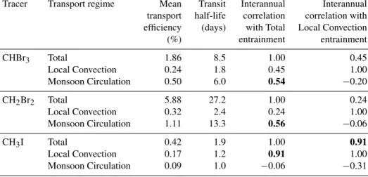
Table 6.Entrainment of CHBr₃, CH₂Br₂, and CH₃I tracer at 17 km altitude through different transport regimes from the west Indian Ocean release box. Correlations with significance of more than 95 % are marked in bold. (Note, transit half-lives differ from Table 4 because of the different model setups.)

Tracer Transport regime Mean Transit Interannual Interannual transport half-life correlation correlation with efficiency (days) with Total Local Convection

(%) entrainment entrainment

CHBr₃ Total 1.86 8.5 1.00 0.45

Local Convection 0.24 1.8 0.45 1.00

Monsoon Circulation 0.50 6.0 0.54 −0.20

CH₂Br₂ Total 5.88 27.2 1.00 0.24

Monsoon Circulation 1.11 13.3 0.56 −0.06

CH₃I Total 0.42 1.9 1.00 0.91

Monsoon Circulation 0.09 1.0 −0.06 −0.31

and CH₃I tracers, the transit half-lives are 8.5, 27.2, and 1.9 days, respectively (Table 6). For the two bromocarbons, the transit time distribution shows two maxima, one for the 0–2 days bin and the second between 4–10 days for CHBr₃ and 6–12 days for CH₂Br₂. CH₃I tracer entrainment occurs mainly on timescales up to 2 days (Fig. 5).

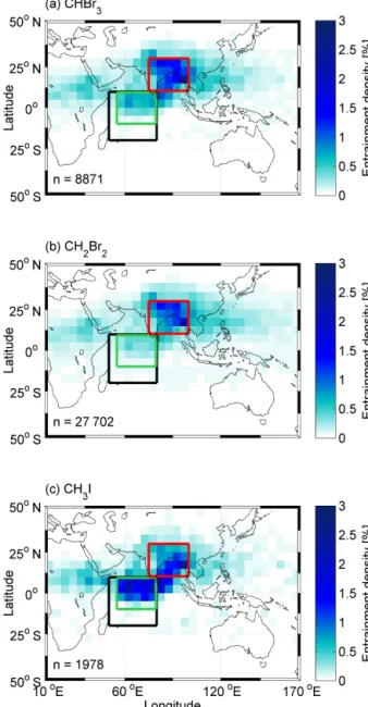
The stratospheric entrainment regions during the Asian summer monsoon between 2000 and 2015 are displayed at the locations where the trajectories first reach 17 km (Fig. 6).

The VSLS tracers show two main entrainment regions. En- hanced entrainment occurs above the Bay of Bengal and northern India in the southeastern part of the Asian monsoon anticyclone and is connected to the Monsoon Circu- lation transport regime (Sect. 3.4). The second entrainment region is above the tropical west Indian Ocean and belongs to the Local Convection regime. We define these two regions to enclose the core entrainment and to be evenly sized in grid space (colored boxes in Fig. 6).

The larger west Indian Ocean release area and longer time series analysis (Table 6) confirms the results of our OASIS analysis (Table 4). The longer-lived VSLS tracers (CHBr3

and CH2Br2)are mainly entrained through the Monsoon Cir- culation regime, while the Local Convection regime is more important for the shortest-lived tracer (CH3I).

Chen et al. (2012) also identified these two stratospheric entrainment regions, analyzing the air transport from the atmospheric boundary layer to the tropopause layer in the Asian Summer monsoon region for a 9-year climatology. Ad- ditionally, they registered entrainment over the west Pacific Ocean, but the Local Convection entrainment above the central Indian Ocean was by far the strongest. Similar to our VSLS transit times, the study of Chen et al. (2012) found very short transport timescales of 0–1 days in the equatorial west Indian Ocean, while transit times above the Bay of Ben- gal and northern India were between 3 and 9 days.

4.2 Interannual variability of stratospheric entrainment

The time series of stratospheric entrainment from the west Indian Ocean to the stratosphere shows interannual variability for all three VSLS tracers (Fig. 7). Overall, July 2014 revealed high entrainment for CHBr3and CH2Br2tracers and low entrainment for CH3I tracer. The coefficient of variation (CV) for total entrainment is 0.13, 0.09, and 0.21 for CHBr3, CH2Br2and CH3I, respectively. Thus, the shortest- lived compound CH3I has the strongest interannual variation, and the longest-lived CH₂Br₂has the weakest variation.

In order to analyze which transport regime has a stronger influence on the total entrainment variability, we correlated the interannual entrainment time series of total entrainment with the entrainment in the Monsoon Circulation and Lo- cal Convection regimes (Table 6). Interannual variability of CHBr₃ and CH₂Br₂ tracer entrainment results mainly from variability in the Monsoon Circulation regime (r=0.54 and r=0.56, respectively). In contrast, the interannual variability of CH₃I tracer entrainment is highly correlated with the Local Convection regime variability (r=0.91). The high variability of total CH3I entrainment (CV=0.21) implies that interannual variation in convection is larger than in the monsoon circulation. The interannual time series of the Mon- soon Circulation and Local Convection regime reveal a weak inverse correlation for all three compounds, suggesting that more entrainment in one regime is related to less entrainment in the other (Fig. 7).

The interannual time series of total VSLS tracer entrainment displays a small increase over time. This increase is independent of the chosen entrainment height (between 13 and 18 km, Fig. S5) and is visible in the analysis for all three tracers. The increase is strongest for CHBr₃and weaker for the other two compounds. It arises mainly from an increase

(13)

Figure 5.VSLS transit time distribution for entrainment at 17 km of (a)CHBr₃,(b)CH₂Br₂, and(c)CH₃I tracers released in July 2000–

2015. Entrained tracer per time interval of 2 days is given as number (gray bars). The blue line gives the cumulative distribution and denotes the transit half-life. The red line shows the decay of the tracers during the transport simulation. The black diamond denotes the transit half-life.

in entrainment in the Monsoon Circulation regime (Fig. 7).

Analyzing changes of rainfall revealed an increase in precipitation over northeastern India for the time interval of our transport study (Latif et al., 2016; Preethi et al., 2016). This indicates an increase in convection in our Monsoon Circula- tion regime over the years from 2000 to 2015, which can ex- plain the increase in stratospheric entrainment. However, for the long time period from the 1950s to the 2010s the same authors found a decrease of precipitation over the above- mentioned area, potentially impacting the VSLS entrainment to the stratosphere.

Figure 6.Density at 17 km of(a)CHBr₃,(b)CH₂Br₂, and(c)CH₃I tracer on a 5^◦×5^◦grid that is released from the west Indian Ocean surface (black box) in July 2000–2015. Colored boxes show the entrainment regions of the Local Convection (green) and Monsoon Circulation (red) regimes.

In a follow-up study we will investigate the influence of the seasonal cycle of the Asian monsoon circulation and interannual influences through atmospheric circulation patterns on the west Indian Ocean VSLS entrainment to the stratosphere in more detail.

5 Uncertainties in the analysis

This study confirms that the subtropical and tropical west Indian Ocean is a source region of oceanic halogenated VSLSs to the stratosphere during the Asian summer mon-

(14)

Figure 7. (a)CHBr₃,(b)CH₂Br₂, and(c)CH₃I tracer entrainment at 17 km from trajectories released from the west Indian Ocean surface box in July 2000–2015. The entrainment is evaluated for three regions: Total, Local Convection, and Monsoon Circulation (see Fig. 6).

soon. The amount of VSLSs entrained depends on the emission strength, the lifetime of the compound, and the transport of trajectories in the regime, which have been quantified in this study.

However, uncertainties of this study are present in various aspects of the analysis. The uncertainties result from the calculation of VSLS emissions, the FLEXPART transport using ERA-Interim reanalysis fields, and the definition of entrainment to the stratosphere.

The calculation of VSLS emissions from the concentration gradient between the ocean at 5 m depth and the atmosphere at 20 m height is subject to measurement uncertainties and a possible different concentration gradient directly at the air–sea interface. Additionally, the applied wind-speed-based parameterization for air–sea flux, which represents a reason- able mean of the published parameterizations, is uncertain by more than a factor of two (Lennartz et al., 2015). Both factors may lead to a systematic flux under- or overestimation in our study.

A vital part of this study is the meteorological reanalysis data from ERA-Interim and the FLEXPART model for determining the VSLS transport. With delivery of our radiosonde launches to the GTS we have improved the data coverage over the Indian Ocean for the time in our study and thus the quality of meteorological reanalysis. Indeed, horizontal wind speed and direction from ship sensors and son- des agree well with the ERA-Interim data (Fig. S2). As the scale of tropical convection is below the state-of-the-art grid scale of global atmospheric models, it is not sufficiently re- solved and must be parameterized. The Lagrangian model FLEXPART uses a convection scheme, described and evaluated by Forster et al. (2007), to account for vertical transport. Using FLEXPART trajectories with ERA-Interim reanalysis, Fuhlbrügge et al. (2016b) were able to simulate VSLS mixing ratios from the surface to the free troposphere up to 11 km above the tropical west Pacific in very good agreement with corresponding aircraft measurements applying a simple source-loss approach. Tegtmeier et al. (2013) showed that the FLEXPART distribution of oceanic CH₃I in the tropics agrees well with adjacent upper tropospheric and lower stratospheric aircraft measurements, thus increas- ing our confidence in the FLEXPART convection scheme and ERA-Interim velocities. Testing different FLEXPART model versions (8.0 and 9.2) for stratospheric entrainment of CHBr₃ (not shown) has revealed only a slightly lower stratospheric entrainment of 0.2 % with the more recent model version 9.2 used in this study here.

Another uncertainty in the location and variability of entrained trajectories may result from the definition of stratospheric entrainment (Sect. 2.2). For the tropics, the cold point tropopause is commonly used as the boundary between the troposphere and the stratosphere (Carpenter et al., 2014). The average measured CPT height during OASIS was 17 km (Fig. S1), but it can be up to 17.6 km high within the Asian monsoon anticyclone during the boreal summer sea- son (Munchak and Pan, 2014). To test the sensitivity of our results with regard to the entrainment height, we analyzed entrained trajectories at several different tropical levels in the upper troposphere/lower stratosphere (UTLS; 13, 15, 17, and 18 km altitude, Fig. S6). As described in Sect. 3.4, we can follow the preferred transport pathways by the migration of maximum density at the intersecting UTLS levels. Analyzing the influence of the application of different UTLS entrainment levels reveals an overall good agreement of interannual variability and long-term changes (Figs. S5 and S6).

6 Summary and conclusion

During the OASIS research cruise in the subtropical and tropical west Indian Ocean in July and August 2014, we conducted simultaneous measurements of the halogenated very short-lived substances, methyl iodide (CH₃I) and for the first time of bromoform (CHBr₃)and dibromomethane