Condensed Matter Physics

Condensed Matter Physics

Vorlesung / Lectures: Monday 09h00 – 11h00

Tuesday 09h00-11h00 Raum / Room: Y36-K-08

https://www.physik.uzh.ch/en/teaching/PHY401/HS2020.html Johan Chang

johan.chang@physik.uzh.ch

Übungen / Exercise class: Tuesday: 11h15 – 13h00 Raum / Room: Y36-K-08

Kevin Kramer

kevin.kramer@uzh.ch

Week Topics

1 Introduction

2 Peierls Instability & CDW order 3 Linear Response theory

4 Magnetism 1: Dia- & Para- magnetism

5 Magnetism 2: Ferro- Anti-Ferro magnetism

7 Correlated Electrons 1: ARPES & Quantum Oscillations 8 Correlated Electrons 2: Mott Physics

9 Correlated Electrons 3: Orbital Physics 10 Superconductivity 1: Landau Theory 11 Superconductivity 2: Vortex Physics 12 Superconductivity 3: Exotic SC

13 Guest lectures 2: Prof. M. Gibert (07.12), Prof. C. Aegeter (13.10) Prof. F. Natterer, Prof. M. Janoschek

Prof. T. Greber

Course Overview Topics

Experimental Cond. Matter.

Guest lectures:

Prof. C. Aegeter (13.10) – Biophysics Prof. M. Gibert (07.12) – Oxide films

Prof. F. Natterer – STM & Single atom magnetism

Prof. M. Janoschek (PSI) – Magnetism & Neutron scattering Prof. T. Greber – Surface science

Prof. J. Osterwalder

Condensed Matter Physics course = 10 ETCS points

30 ETCS points per semester ⟹ 10 ETCS points ≈ 12 hours per week

Practical information

Lectures + Ex. Class Reading / Studying Solve Exercises

6 hours ~3 hours ~3 hours

Proposed work-load distribution

Strategy / Advice

(1) Solve the exercises your self.

(2) Read and study continuously

(3) Be active during the lecture and exercise class

Your task for this week

For next week

(1) Read Kittel – “Peierls Instability of Linear Metals”

Chapter 10 (2) Read notes.

(3) Checkout the exercise sheet on the course webpage.

Chapter 1:

Crystal Structures

Concepts:

Lattice + Basis = crystal structure

Chapter 2:

Crystal Structures Determination

8. Scattering theory & Experiments

Concept 8.0.1 — Fermi Golden Rule. Let’s consider an initial quantum mechanical state y _i = | i i and image it is exposed to a potential V ( r ) . Now, we let y _f = | f i be an arbitrary final state. The Fermi golden rule (not proven here) allows evaluation of the transition rate – i.e. the transition probability ( | i i ! | f i ) per time

P = 2p

h ¯ | h f | V | i i | ² d (E _f E _i ) where h f | V | i i =

Z d ~ ry _f V ( ~ r) y _i . (8.1)

Here d is the delta-function and E _f and E _i are the energy of the initial and final states.

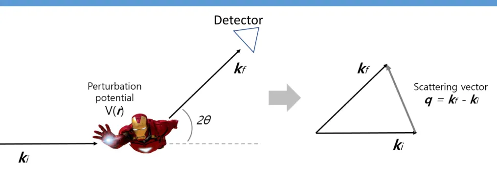
Concept 8.0.2 — Elastic Scattering. In a scattering experiment, an incident particle is scattered on an object that is modeled by some potential V ( ~ r) . Let’s assume that the incident and scattered particle can be described by plane waves y µ exp (i ~ k ~ r) . This is correct as long as the particle source and final detector is sufficiently far from the scattering object. In the following, we will consider only elastic scattering. That is, the energy of initial and final state is identical

Figure 8.1: Scattering triangle. (a) Incident particle with momentum ~ k _i scattering on an object with a scattering angle defined as 2q . The resulting momentum is defined as ~ k _f ( f for final). (b) Another representation of the scattering triangle defining the scattering vector ~ q = ~ k _f ~ k _i .

Detector

Concepts:

Form & Structure factor

Reciprocal space

3.3 Techniques

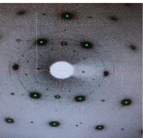
Beam alignment: In order to observe the di↵erent Bragg peaks with the point detector, the sample has to be aligned. This is usually done by detecting the di↵raction pattern with the 2D detector. First the sample has to be turned around the high-order axis until a high symmetry plane is found. After noting the position, the sample is mounted in the desired environment, e.g. the cryostat magnet. The previous plane is found again. Then, a Bragg peak has to be chosen and brought into the possible scanning direction (green line on Fig. 3.4 by tilting the sample. Usually, peak splitting is observed best at a high order peak (peaks with high Miller plane indices), but those peaks also tend to be less intensive due to the scattering geometry.

Thus one has to compromise by finding a high order peak that is still intense enough.

Figure 3.4: 2D detector image used for alignment. Non-aligned high symmetry plane of sample inside a magnet. The dark points are Bragg peaks, while the bright circle in the center is the projection of a beam stopper. The green dots inside the dark ones means that the detector is about to be oversaturated. The red line shows the possible scanning direction. The dark circular structures around the beam stopper are powder di↵raction rings coming from the aluminum window.

Superconducting Magnet Crysostat: In order to cool the sample down to temperatures around 3 K, we used the superconducting magnet cryostat shown in Fig. 3.6a). The magnet was also used to produce horizontal magnetic fields of up to 10 T.

Pressure Cell: Our experiment demanded a device which applies hydrostatic pressure on the sample and which is small enough to fit in the magnet cryostat. A pressure cell with the desired dimensions was filled with oil and then used to contain the sample. A hydraulic press as shown in Fig. 3.6b) was used to load the pressure and gave a rough estimate on the pressure inside. To obtain the exact pressure, a special property of the cuprate perovskite material La

2-x

Ba

x

CuO

4

was used: By applying pressure on the material, the crystal structure transists from two-fold symmetry to four-fold symmetry [11]. In reciprocal lattice space this correspond to a merging of two Bragg peaks as shown in Fig. 3.5a). The peak splitting q can be mapped to the applied pressure and fitted with a curve as shown in Fig. 3.5b).

In our case, an ! scan was done over the (0 2 0) lattice position (tetragonal notation). The intensity of the Bragg peaks was measured against ! and the data fitted with two Lorenzian functions as shown in Fig. 3.5b. The di↵erence in angle of the two peak positions was then

30

Chapter 2:

Crystal Structures Determination

Single crystal Powder

Bachelor thesis: Nik Dennler

https://www.diamond.ac.uk/industry/Industry-News/Latest- News/Synchrotron-Industry-News-Powder-Diffraction.html

Chapter 3:

Crystal Bindings

Concepts:

Attractive

Repulsive interaction

Binding energy

Chapter 3:

Crystal Bindings – Thermal Expansion

Chapter 3:

Crystal Bindings – Thermal Expansion

Chapter 3:

Crystal Bindings – Negative Thermal Expansion

for Ca

₂

Ru

_0.90

Cu

_0.10

O

₄

(Cu0.10). Particularly, the Fe-doped ruthenate exhibits

T-linear expansion in almost the entire range

of

T

below 500 K, which is favourable for practical applications.

Thermal expansion exhibits almost

T-linear behaviour, even near

the lowest temperature (95 K) used for the present dilatometry measurements. Therefore, NTE apparently continues down to the lower temperature. In that case, the total volume change

DV/V

might become greater than the present estimate of 2.8%

(T

¼

95–500 K).

Effects of oxygen deficiency. We can examine the differences

between the present materials showing giant NTE and previous materials. Figure 2 shows linear thermal expansion

DL(T)/L

of reduced (#1), oxidized (#2), and re-reduced (#3) Ca

2

RuO

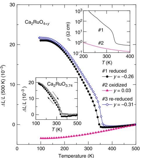
4

in the present experiments (see ‘Methods’ section for sample prepara- tion conditions). The giant NTE of the reduced sample is suppressed dramatically by high-pressure oxidizing procedures.

When this oxidized sample is reduced again, the giant NTE is recovered. The results presented above imply that differences in oxygen contents produce a striking difference in thermal- expansion properties. Evaluations of the oxygen contents by thermogravimetric analysis are

y¼ "

0.26(1), 0.03(1) and

"

0.31(1), respectively, for the reduced, oxidized and re-reduced samples in the notation of Ca

₂

RuO

_4þy

. Reports of an earlier study described that

y

fell within the range of

"

0.01(1) to

þ

0.07(1)

¹⁵

. The present reduced ruthenates are regarded as having larger amounts of oxygen deficiency than the previous ones. Hereinafter, we use Ca

₂

Ru

_1"xM_x

O

_4þy

notation as the present materials. The

y

values are presented in Table 2.

High-temperature L to low-temperature S phase transition.

The giant NTE of Ca

₂

RuO

_3.74

seems to be triggered by the transition from the high-T metallic L phase to the low-T insu- lating S phase. The inset of Fig. 2 presents the temperature dependence of resistivity

r(T) for the reduced and oxidized

Ca

₂

RuO

_4þy

. The resistivity of the reduced sample indicates that the system undergoes the MI transition at

T_MI¼

345 K. The onset of NTE is almost identical to this MI transition. In contrast, resistivity of the oxidized sample shows no abrupt change that can be interpreted as prolonged high-T L phase down to lower temperatures. Corresponding to this MI transition, the anomaly appears in the magnetic susceptibility

w

(T) (Supplementary Fig. 2).

w

(T) is hysteretic (

B

10 K). It therefore supports the first-order nature of this phase transition. Such hysteretic beha- viour is confirmed also in the linear thermal expansion. The hysteresis loop was observed in dilatometry measurements (inset of Fig. 2). The onset of NTE is 340 and 355 K on cooling and warming processes, respectively. This loop behaviour is partly attributable to the first-order phase transition. The loop behaviour is reproducible through several successive measure- ments.

Structural characterization of Ca₂Ru_1"xM_xO_4þy

. Giant NTE can be considered in terms of its crystal structure. The XRD profiles were refined using Le Bail method by RIETAN-FP

²⁵

(Supplementary Figs 3 and 4). The structural parameters such as

Table 1 | Parameters related to negative thermal expansion for recently discovered giant negative thermal-expansion materials.

DV/V(%) TNTE(K) DT(K) a (10^"6K^"1)^* Structure^w Method^z Reference

ZrW₂O₈ 1.2 o425 425 "9 Cubic D/N ⁶

Cd(CN)₂ 2.1 170–375 205 "34 Cubic X ⁷

Mn3Ga0.7Ge0.3N0.88C0.12 0.5 197–319 122 "18 Cubic D ⁹

LaFe10.5Co1.0Si1.5 1.1 240–350 110 "26 Cubic D ¹⁰

MnCo0.98Cr0.02Ge 3.2 122–332 210 "52 Orthorhombic D ¹¹

SrCu3Fe4O12 0.4 180–250 70 "20 Cubic X ¹²

Bi_0.95La_0.05NiO₃ 2.0 320–380 60 "82 Triclinic D ¹³

0.4PbTiO₃–0.6BiFeO₃ 2.7 298–923 625 "13 Tetragonal X ¹⁴

Pu 5.4 337–480^y — — Cubic/Tetragonal D ²³

YMn2 4.7 75^|| — — Cubic X ²⁴

Parameters of materials with phase transition accompanied by large volume contraction on heating, not broadened, are also listed for comparison.

*Averaged value when the material is anisotropic.

wFor NTE region or lower temperature, larger-volume phase.

zD, dilatometry; N, neutron diffraction; X, X-ray diffraction.

ySuccessive transitions.

||In warming process.

0 100 200 300 400 500

0 10 20 30

Temperature (K)

!L/L (500 K) (10–3 )

Ca₂RuO_4+y

#1 reduced

#2 oxidized

#3 re-reduced y = –0.26 y = 0.03 y = –0.31

200 300 400

10^–1 10⁰ 10¹ 10² 10³

T (K)

" (Ωcm) #1

#2

0 10 20

T (K)

!L/L (10–3 ) Ca₂RuO_3.74

100 300 500

Figure 2 | Linear thermal expansion DL/Lof Ca₂RuO_4þy.The data were collected on a warming process using a laser-interference dilatometer.

Reference temperature: 500 K. The hysteresis loop was observed in DL/L measurements using a thermomechanical analyzer for #1 (inset). The giant negative thermal expansion (NTE) of #1 is suppressed by the oxidizing procedure, but is fully recovered by the re-reducing procedure. Inset shows temperature dependence of resistivity r(T) for #1 and #2. The abrupt jump in r(T) at 345 K for #1 corresponds to the Mott metal-to-insulator transition, which coincides with the onset of NTE.

NATURE COMMUNICATIONS | DOI: 10.1038/ncomms14102

ARTICLE

NATURE COMMUNICATIONS| 8:14102 | DOI: 10.1038/ncomms14102 | www.nature.com/naturecommunications 3

ARTICLE

Received 10 Mar 2016 | Accepted 28 Nov 2016 | Published 10 Jan 2017

Colossal negative thermal expansion in reduced layered ruthenate

Koshi Takenaka ¹ , Yoshihiko Okamoto ^1,2 , Tsubasa Shinoda ¹ , Naoyuki Katayama ¹ & Yuki Sakai ³

Large negative thermal expansion (NTE) has been discovered during the last decade in materials of various kinds, particularly materials associated with a magnetic, ferroelectric or charge-transfer phase transition. Such NTE materials have attracted considerable attention for use as thermal-expansion compensators. Here, we report the discovery of giant NTE for reduced layered ruthenate. The total volume change related to NTE reaches 6.7% in dilato- metry, a value twice as large as the largest volume change reported to date. We observed a giant negative coefficient of linear thermal expansion a ¼ " 115 # 10 ^{" 6} K ^{" 1} over 200 K interval below 345 K. This dilatometric NTE is too large to be attributable to the crystal- lographic unit-cell volume variation with temperature. The highly anisotropic thermal expansion of the crystal grains might underlie giant bulk NTE via microstructural effects consuming open spaces in the sintered body on heating.

DOI: 10.1038/ncomms14102 OPEN

1 Department of Applied Physics, Nagoya University, Furo-cho, Chikusa-ku, Nagoya 464-8603, Japan. ² Institute for Advanced Research, Nagoya University, Furo-cho, Chikusa-ku, Nagoya 464-8601, Japan. ³ Kanagawa Academy of Science and Technology, KSP, 3-2-1 Sakado, Takatsu-ku, Kawasaki 213-0012, Japan.

Correspondence and requests for materials should be addressed to K.T. (email: takenaka@nuap.nagoya-u.ac.jp).

NATURE COMMUNICATIONS | 8:14102 | DOI: 10.1038/ncomms14102 | www.nature.com/naturecommunications 1

Chapter 4:

Lattice Vibrations - Phonons

Concepts:

Phonon modes

Transverse and Longitudinal modes

Discrete wave numbers k

Chapter 5:

Lattice Vibrations – Heat Capacity

Concepts:

Density of states DOS Heat capacity C=dU/dT Response: CdT=dU

Phonon Heat Capacity

C=𝛼𝑇 ^% (T→ 0)

Chapter 6:

Free Electron Gas– Heat Capacity

ARTICLES NATURE PHYSICS DOI: 10.1038/NPHYS1921

30 35 40 45

¬2 0 2

¬2 0 2

¬2 0 2

¬2 0 2

H (T)

∆C p (mJ mol¬1 K¬1 ) ∆C p (mJ mol¬1 K¬1)

∆Cp (mJ mol¬1 K¬1)

5.5 K

~3 K 2 K 1 K I

II

III

IV 1

2 3 4 5

6 32 34 36 38 40 42 44

Temperature (K)

¬1.60

¬1.30

¬1.10

¬0.85

¬0.60

¬0.36

¬0.11 0.140.39 0.630.88 1.101.40 1.60

H (T) 1.6

0.8 0

¬0.830

34 38 H (T)

42

46 6 5 4 3 Tempera

ture (K)

2 1 0

a

c

b

Figure 2 | Oscillatory component of electronic specific heat. a, Equation (1) for a single 531 ± 3 T pocket with warping of 15.2 ± 0.5 T. Note the location of the node depends only on m

^⇤

. For YBCO 6.56, we find m

^⇤

= 1.34 ± 0.06 m

_e

. b, Oscillatory component of data (circles) with the a fit superimposed (black lines). Blue/cyan data at 1 K result from sweeping the magnetic field up/down and show no hysteresis. The dashed line demonstrates the ⇡ -phase shift between 2 K and 5.5 K. c, Temperature-field plot of a, with coloured lines indicating locations of the data shown in b.

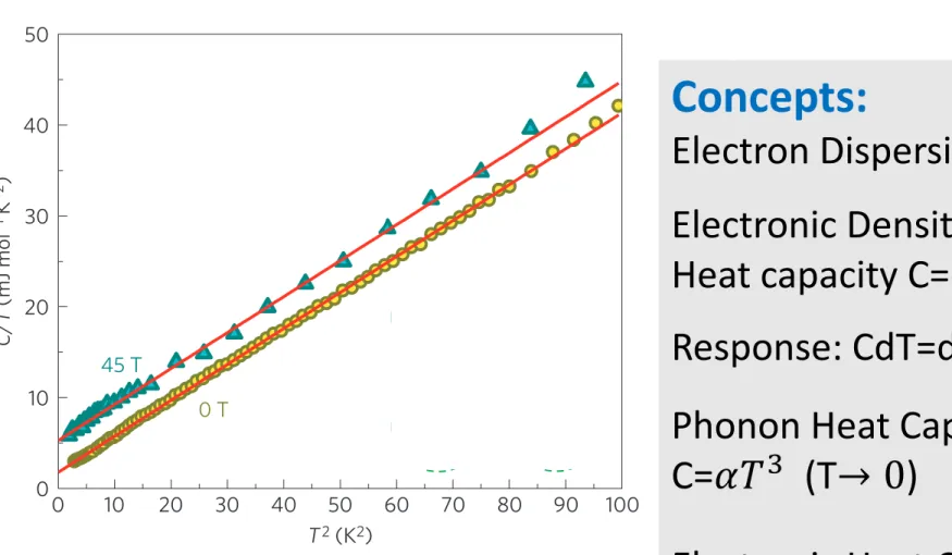
For a two-dimensional Fermi liquid with parabolic bands, in which the density of states is constant, the total electronic contribution to the specific heat is a simple sum over each piece or pocket of the Fermi surface:

total

=

⁰

X

i

n

i

m

i⇤

/ m

e

(2) where n is the number (multiplicity) of the ith-type of pocket in the first Brillouin zone (BZ), m

i⇤

is the effective mass of the ith-type of pocket, and

⁰

= 1.46 mJ mol

¹

K

²

. (A similar expression holds for Dirac-like dispersion with an appropriate redefinition of m

^⇤

; see Supplementary Information.) Within the scenario in which the high-field resistive state is interpreted as a normal state Fermi liquid, a single pocket in the first BZ (n = 1; m

^⇤

= 1 . 35 m

e

) would yield

total

= 1.9 mJ mol

¹

K

²

and a single pocket per CuO

2

plane (that is n = 2; m

^⇤

= 1 . 35 m

e

) would yield

total

= 3 . 8 mJ mol

¹

K

²

. The symmetry of the BZ admits only two possibilities for a single pocket, both of which are shown in the upper left of Fig. 3. Among other scenarios, it has been proposed that the high-field resistive state in underdoped YBCO is a spin density wave with a Fermi surface reconstruction (lower right inset of Fig. 3), where there is one pocket per CuO

2

plane centred at ( ± ⇡; 0)(0; ± ⇡) with m

^⇤

= 1 . 35 m

e

and two pockets at (⇡/2; ⇡/2) with m

^⇤

= 3.8 m

e

(ref. 3) which would yield

total

= 26 mJ mol

¹

K

²

(see Supplementary Information).

Interestingly, this simple Fermi surface pocket counting scheme works well in the case of overdoped Tl

2

Ba

2

CuO

6+

(T

c

= 10 K), where transport quantum oscillations experiments found a single frequency with an effective mass of m

^⇤

= 4 . 9 m

e

, predicting of 7 . 2 mJ mol

¹

K

²

(ref. 27). Specific heat measurements made on overdoped Tl

2

Ba

2

CuO

6+

with T

c

= 10 K have indeed independently determined ⇡ 7 mJ mol

¹

K

²

(ref. 28). In the underdoped YBCO measurements reported here, the observed value of = 1 . 85 mJ mol

¹

K

²

in Fig. 1 is too small to be consistent with the Fermi surface reconstruction scenario suggested from early quantum oscillation measurements

^2,3

. The persistence of

0 10 20 30 40 50 60 70 80 90 100

0 10 20 30 40 50

C/T (mJ mol¬1 K¬2 )

T² (K²) 45 T

0 T (0, 0)

(π, π)

Figure 3 | Temperature dependence of the specific heat. a, C/T versus T

²

for H = 0 T (yellow circles) and H = 45 T (blue triangles). Both the

zero-field superconducting state and high-field resistive state look

Fermi-liquid-like, with contributions from (linear) electronic and (cubic) phonon terms. The phonon term is independent of field with slope

= 0.395 mJ mol

¹

K

⁴

. Upper left schematics are Fermi surfaces for which symmetry allows a single pocket that is centred at (0, 0) or (⇡,⇡).

Lower right schematic represents the Fermi surface reconstruction

described in the text, for which

_total

= 26 mJ mol

¹

K

²

for one electron pocket and two hole pockets per CuO

₂

plane (see

Supplementary Information).

the p

H signature of a d -wave superconducting gap would seem to rule out an interpretation in which the high magnetic field destroys the said d -wave gap to reveal a conventional normal state Fermi liquid.

Thus, we turn attention to the second scenario in which the state in a high magnetic field is a vortex liquid, which features the coexistence of Fermi liquid quasiparticles and mobile

334

NATURE PHYSICS | VOL 7 | APRIL 2011 | www.nature.com/naturephysics

© 2011 Macmillan Publishers Limited. All rights reserved

Concepts:

Electron Dispersion

Electronic Density of States Heat capacity C=dU/dT

Response: CdT=dU

Phonon Heat Capacity C=𝛼𝑇 ^% (T→ 0)

Electronic Heat Capacity

C=γ𝑇 (T→ 0)

Chapter 7:

Electronic Band Structure

Concepts:

Bloch’s Theorem Band Structure Fermi Surface &

Fermi momentum

Electronic material classification

Linear chain -Models

Structure factor: S = ∑ 𝒆 _𝒊 ^{+𝒊𝒒𝒓 𝒊}

Madelungs constant: 𝜶 = 𝟐 𝒍𝒏(𝟐)

Distortion Energy : 𝑬 = 𝟎. 𝟓 ∗ 𝒄𝒐𝒏𝒔𝒕𝒂𝒏𝒕 ∗ 𝜹 ^𝟐

Phonon dispersion: 𝛚 =