Conformalinvarianceoftransverse-momentumdependentpartondistributionsrapidityevolution PHYSICALREVIEWD 100, 051504(R)(2019)

Conformal invariance of transverse-momentum dependent parton distributions rapidity evolution

Ian Balitsky

Physics Department, Old Dominion University, Norfolk, Virginia 23529, USA and Theory Group, JLAB, 12000 Jefferson Avenue, Newport News, Virginia 23606, USA

Giovanni A. Chirilli

Institut für Theoretische Physik, Universität Regensburg, D-93040 Regensburg, Germany

(Received 17 June 2019; published 20 September 2019)

We discuss conformal properties of TMD operators and present the result of the conformal rapidity evolution of TMD operators in the Sudakov region.

DOI: 10.1103/PhysRevD.100.051504

I. INTRODUCTION

In recent years, the transverse-momentum dependent parton distributions (TMDs) [1 – 4] have been widely used in the analysis of processes like semi-inclusive deep inelastic scattering or particle production in hadron-hadron collisions (for a review, see Ref. [5]).

The TMDs are defined as matrix elements of quark or gluon operators with attached lightlike gauge links (Wilson lines) going to either þ∞ or −∞ depending on the process under consideration. It is well known that these TMD operators exhibit rapidity divergencies due to infinite lightlike gauge links and the corresponding rapidity/UV divergences should be regularized. There are two schemes on the market: the most popular is based on Collins-Soper- Sterman [2] or soft-collinear effective theory [6] formalism, and the second one is adopted from the small-x physics [7,8]. The obtained evolution equations differ even at the leading-order level and need to be reconciled, especially in view of the future electron-ion collider accelerator which will probe the TMDs at values of Bjorken x between small- x and x ∼ 1 regions.

In our opinion, a good starting point is to obtain conformal leading-order evolution equations. It is well known that at the leading-order perturbative QCD (pQCD) is conformally invariant, so there is hope of get any evolution equation without explicit running coupling from conformal considerations. In our case, since TMD oper- ators are defined with attached lightlike Wilson lines, formally they will transform covariantly under the sub- group of the full conformal group which preserves this lightlike direction. However, as we mentioned, the TMD

operators contain rapidity divergencies which need to be regularized. At present, there is no rapidity cutoff which preserves conformal invariance, so the best one can do is to find the cutoff which is conformal at the leading order in perturbation theory. In higher orders, one should not expect conformal invariance since it is broken by the running of QCD coupling. However, if one considers corresponding correlation functions in N ¼ 4 super Yang-Mills (SYM), one should expect conformal invariance. After that, the results obtained in N ¼ 4 SYM theory can be used as a starting point of QCD calculation. Typically, the result in N ¼ 4 theory gives the most complicated part of the pQCD result, i.e., the one with maximal transcendentality. Thus, the idea is to find the TMD operator conformal in N ¼ 4 SYM and use it in QCD. This scheme was successfully applied to the rapidity evolution of color dipoles. At the leading order, the Balitsky-Kovchegov evolution of color dipoles [9 – 12] is invariant under SL(2,C) (Möbius) group.

At the next-to-leading order (NLO), the “ conformal dipole ” with the α s correction [13] makes NLO Balitsky- Kovchegov evolution Möbius invariant for N ¼ 4 SYM, and the corresponding QCD kernel [14] differs by terms proportional to the β function.

II. CONFORMAL INVARIANCE OF TMD OPERATORS

For definiteness, we will talk first about gluon operators with lightlike Wilson lines stretching to −∞ in the þ direction. The gluon TMD (unintegrated gluon distribution) is defined as [15]

Dðx B ;k

_⊥

; ηÞ¼ Z

d

²

z

_⊥

e ^iðk;zÞ

^⊥

Dðx B ;z

_⊥

; ηÞ;

g

²

Dðx B ;z

_⊥

; ηÞ¼ − x

⁻¹

_B 2π p

⁻

Z

dz

^þ

e

^−ixB

^p

⁻

^z

^þ

×hPjF ^a

_ξ

ðzÞ½z −∞ n; −∞ n ^ab F ^bξ ð0ÞjPij z

⁻¼0

; ð1Þ Published by the American Physical Society under the terms of

the Creative Commons Attribution 4.0 International license.

Further distribution of this work must maintain attribution to the author(s) and the published article ’ s title, journal citation, and DOI. Funded by SCOAP

³

.

Rapid Communications

where jPi is an unpolarized target with momentum p ≃ p

⁻

(typically proton) and n ¼ ð

¹

ffiffi

p2

; 0 ; 0 ;

¹

ffiffi

p2

Þ is a lightlike vector in the “þ” direction. Hereafter, we use the notation

F

^ξ;a

ðz

_⊥

; z

^þ

Þ ≡ gF

^−ξ;m

ðzÞ½z; z − ∞ n ^ma j _z

−¼0

; ð2Þ where ½x; y denotes straight-line gauge link connecting points x and y:

½x; y ≡ Pe ^ig

R duðx

−

yÞ

^μ

A

_μðuxþð1−

uÞyÞ

: ð3Þ

To simplify one-loop evolution, we multiplied F

_μν

by a coupling constant. Since the gA

_μ

is renormalization invari- ant, we do not need to consider self-energy diagrams (in the background-Feynman gauge). Note that z

⁻

¼ 0 is fixed by the original factorization formula for particle production [5]

(see also the discussion in Refs. [16,17]).

The algebra of full conformal group SOð2 ; 4Þ consists of four operators P

^μ

, six M

^μν

, four special conformal gen- erators K

^μ

, and dilatation operator D. It is easy to check that in the leading order the following 11 operators act on gluon TMDs covariantly,

P ⁱ ; P

⁻

; M

¹²

; M

⁻ⁱ

; D; K ⁱ ; K

⁻

; M

^−þ

; ð4Þ while the action of operators P

^þ

, M

^þi

, and K

^þ

do not preserve the form of the operator (2). The action of the generators (4) on the operator (2) is the same as the action on the field F

⁻ⁱ

without gauge link attachments. The corre- sponding group consists of transformations which leave the hyperplane z

⁻

¼ 0 and vector n invariant. Those include shifts in transverse and þ directions, rotations in the trans- verse plane, Lorentz rotations/boosts created by M

⁻ⁱ

, dila- tations, and special conformal transformations

z

⁰_μ

¼ z

_μ

− a

_μ

z

²

1 − 2 a · z þ a

²

z

²

ð5Þ with a ¼ ða

^þ

; 0; a

_⊥

Þ. In terms of “embedding formalism”

[18 – 21] defined in six-dimensional space, this subgroup is isomorphic to the “ Poincar´e þ dilatations ” group of the four- dimensional subspace orthogonal to our physical lightlike þ and “−” directions.

As we noted, infinite Wilson lines in the definition (2) of TMD operators make them divergent. As we discussed above, it is very advantageous to have a cutoff of these divergencies compatible with approximate conformal invariance of tree-level QCD. The evolution equation with such a cutoff should be invariant with respect to trans- formations described above.

In the next section, we demonstrate that the “ small-x ” rapidity cutoff enables us to get a conformally invariant evolution of TMD in the so-called Sudakov region.

III. TMD FACTORIZATION IN THE SUDAKOV REGION

The rapidity evolution of the TMD operator (1) is very different in the region of large and small longitudinal separations z

^þ

. The evolution at small z

^þ

is linear and double-logarithmic, while at large z

^þ

, the evolution becomes nonlinear due to the production of color dipoles typical for small-x evolution. It is convenient to consider as a starting point the simple case of TMD evolution in the so- called Sudakov region corresponding to small longitudinal distances.

First, let us specify what we call a Sudakov region. A typical factorization formula for the differential cross section of particle production in hadron-hadron collision is [5,22]

dσ

d η d

²

q

_⊥

¼ X

f

Z

d

²

b

_⊥

e ^iðq;bÞ

^⊥

D f=A ðx _A ;b

_⊥

; ηÞ

× D f=B ðx _B ;b

_⊥

; ηÞσðff → HÞþ; ð6Þ where η ¼

¹₂

ln ^q _q

^þ−

is the rapidity, D f=h ðx; z

_⊥

; ηÞ is the TMD density of a parton f in hadron h, and σðff → HÞ is the cross section of production of particle H of invariant mass m

²

_H ¼ q

²

≡ Q

²

in the scattering of two partons. (One can keep in mind Higgs production in the approximation of the pointlike gluon-gluon-Higgs vertex). The Sudakov region is defined by Q ≫ q

_⊥

≫ 1 GeV since at such kinematics there is a double-log evolution for transverse momenta between Q and q

_⊥

. In the coordinate space, TMD factorization (6) looks like

hp _A ; p _B jg

²

F ^a

_μν

F ^aμν ðz

₁

Þg

²

F ^b

_λρ

F ^bλρ ðz

₂

Þjp _A ; p _B i

¼ 1

N

²

_c − 1 hp A j O ˜ ij ðz

⁻₁

; z

_1⊥

; z

⁻₂

; z

_2⊥

Þjp A i

^σA

× hp _B jO ^ij ðz

^þ₁

; z

_1⊥

; z

^þ₂

; z

_2⊥

Þjp _B i

^σB

þ ; ð7Þ where

O ij ðz

^þ₁

; z

_1⊥

; z

^þ₂

; z

_2⊥

Þ ¼ F ^a _i ðz

₁

Þ½z

₁

− ∞ n; z

₂

− ∞ n ^ab

× F ^b _j ðz

₂

Þj _z

−

1¼z⁻₂¼0

; ð8Þ

O ˜ ij ðz

⁻₁

; z

_1⊥

; z

⁻₂

; z

_2⊥

Þ ¼ F ^a _i ðz

₁

Þ½z

₁

− ∞ n

⁰

; z

₂

− ∞ n

⁰

^ab

× F ^b j ðz

₂

Þj _z

^þ

1¼z^þ₂¼0

;

F ^i;a ðz

_⊥

; z

⁻

Þ ≡ gF

^þi;m

ðzÞ½z; z − ∞n

⁰

^ma j _z

^þ_¼0

: ð9Þ

Here, p _A ¼ ffiffi _s

2

p nþ ^p ffiffiffiffi

^2A

p2s

n

⁰

, p _B ¼ ffiffi

2

s

q n

⁰

þ ^p ffiffiffiffi

^2B

p2s

n, and n

⁰

¼ ð

¹

ffiffi

p2

; 0 ; 0; −

¹

ffiffi

p2

Þ. Our metric is x

²

¼ 2x

^þ

x

⁻

− x

²_⊥

.

As we mentioned, TMD operators exhibit rapidity divergencies due to infinite lightlike gauge links. The

“small-x style” rapidity cutoff for longitudinal divergencies

is imposed as the upper limit of k

^þ

components of gluons

emitted from the Wilson lines. As we will see below, to get

the conformal invariance of the leading-order evolution, we

need to impose the cutoff of k

^þ

components of gluons correlated with transverse size of TMD in the following way:

F ^i;a ðz

_⊥

; z

^þ

Þ

^σ

≡ gF

^−i;m

ðzÞ½Pe ^ig R

_zþ

−∞

dz

^þ

A

^−;σðup₁þx_⊥Þ

^ma ; A

^σ_μ

ðxÞ ¼

Z d

⁴

k 16π

⁴

θ

σ ffiffiffi p 2 z

_12⊥

− jk

^þ

j

e

^−ik·x

A

_μ

ðkÞ:

ð10Þ Similarly, the operator O ˜ in Eq. (9) is defined with with the rapidity cutoff for β integration imposed as θð

^σ˜

ffiffi

p2

z

_12⊥

− jk

⁻

jÞ.

The Sudakov region Q

²

≫ q

²_⊥

in the coordinate space corresponds to

z

²_12k

≡ 2 z

⁻₁₂

z

^þ₁₂

≪ z

²₁₂

⊥

; ð11Þ

where z

₁₂

≡ z

₁

− z

₂

. In the leading log approximation, the upper cutoff for k

^þ

integration in the target matrix element in Eq. (7) is σ B ¼

¹

ffiffi

p2

z

_12⊥

z

⁻₁₂

, and similarly the β -integration cutoff in the projectile matrix element is σ A ¼

¹

ffiffi

p2

z

_12⊥

z

^þ₁₂

[23].

In the next section, we demonstrate that the rapidity cutoff (10) enables us to get a conformally invariant evolution of TMD in the Sudakov region (11).

IV. ONE-LOOP EVOLUTION OF TMDS A. Evolution of gluon TMD operators in

the Sudakov region

In this section, we derive the evolution of gluon TMD operator (8) with respect to cutoff σ in the leading log approximation. As usual, to get an evolution equation, we integrate over momenta

^σ2

ffiffi

2 p

z

_12⊥

> k

^þ

>

^σ1

ffiffi

2 p

z

_12⊥

. To this end, we calculate diagrams shown in Fig. 1 in the background field of gluons with k

^þ

<

^σ1p

ffiffi

₂

z

_12⊥

. The calculation is easily done by method developed in Refs. [24,25], and the result is

O

^σ2

ðz

^þ₁

; z

^þ₂

Þ ¼ α s N _c 2π

σ

Z

2^p

ffiffi

₂

z12⊥

σ1^p

ffiffi

₂

z12⊥

dk

^þ

k

^þ

K O

^σ1

ðz

^þ₁

; z

^þ₂

Þ; ð12Þ

where the kernel K is given by K Oðz

^þ₁

; z

^þ₂

Þ ¼ Oðz

^þ₁

; z

^þ₂

Þ

Z _z

þ 1

−∞

dz

^þ

z

^þ₂

− z

^þ

e

⁻ⁱ

z12⊥σ

ffiffi

2 pðz2−zÞþ

þ Oðz

^þ₁

; z

^þ₂

Þ Z _z

þ

2

−∞

dz

^þ

z

^þ₁

− z

^þ

e ⁱ

z12⊥σ

ffiffi

2 pðz1−zÞþ

− Z _z

þ

1

−∞

dz

^þ

Oðz

^þ₁

; z

^þ₂

Þ − Oðz

^þ

; z

^þ₂

Þ z

^þ₁

− z

^þ

− Z z

^þ₂

−∞

dz

^þ

Oðz

^þ₁

; z

^þ₂

Þ − Oðz

^þ₁

; z

^þ

Þ

z

^þ₂

− z

^þ

; ð13Þ

where we suppress arguments z

_1⊥

and z

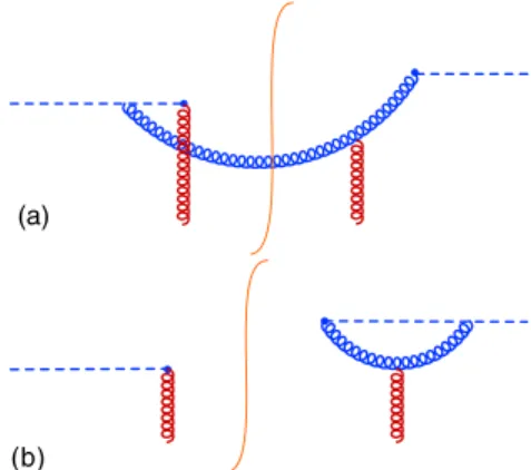
_2⊥

since they do not change during the evolution in the Sudakov regime. The first two terms in the kernel K come from the “ production ” diagram in Fig. 1(a), while the last two terms come from the

“virtual” diagram in Fig. 1(b). The result (13) can be also obtained from Ref. [25] by Fourier transformation of Eq. (5.9) with the help of Eqs. (3.12) and (3.30) therein.

The approximations for diagrams in Fig. 1 leading to Eq. (13) are valid as long as

k

^þ

≫ z

^þ₁₂

z

²₁₂

⊥

; ð14Þ

which gives the region of applicability of Sudakov-type evolution.

Evolution equation (12) can be easily integrated using Fourier transformation. Since

Ke

^−ik−

^z

^þ1þik0−

^z

^þ2

¼

−2 ln σ z

_12⊥

− lnðik

⁻

Þ − lnð− ik

⁰⁻

Þ þ ln 2 − 4γ E þ O

z

^þ₁₂

z

_12⊥

σ

e

^−ik−

^z

^þ1þik0−

^z

^þ2

; ð15Þ one easily obtains

O

^σ2

ðz

^þ₁

; z

^þ₂

Þ ¼ e

^−2¯αsln

σ2

σ1½lnσ1σ2þ4γE−ln2

× Z

dz

^0þ₁

dz

^0þ₂

O

^σ1

ðz

^0þ₁

; z

^0þ₂

Þz

^−2¯αsln

σ2 σ1

12⊥

× 1 4π

²

"

i Γð1 − 2¯ α s ln

^σ_σ²

1

Þ

ðz

^þ₁

− z

^0þ₁

þ iϵÞ

^{1−2¯αslnσσ21}

þ c:c:

#

×

"

i Γð1 − 2¯ α s ln

^σ_σ²

1

Þ

ðz

^þ₂

− z

^0þ₂

þ i ϵÞ

^{1−2¯αslnσσ21}

þ c:c:

#

; ð16Þ

where we introduced notation α ¯ s ≡

^αs_4π

^N

^c

. It should be mentioned that the factor 4γ E is “ scheme dependent ” ;

(a)

(b)

FIG. 1. Typical diagrams for production (a) and virtual (b) con-

tributions to the evolution kernel. The dashed lines denote gauge

links.

if one introduces to α integrals smooth cutoff e

^−α=a

instead of rigid cutoff θða > αÞ, the value 4γ E changes to 2γ E .

It is easy to see that the rhs of Eq. (16) transforms covariantly under all transformations (4) except the Lorentz boost generated by M

^þ−

. The reason is that the Lorentz boost in the z direction changes cutoffs for the evolution.

To understand that, note that Eq. (15) is valid until σ > ^z

þ 12

z

²₁₂

⊥

, so the linear evolution (16) is applicable in the region between

σ

₂

¼ σ B ¼ z

_12⊥

z

⁻₁₂

ffiffiffi

p 2 and σ

₁

¼ z

^þ₁₂

ffiffiffi p 2

z

_12⊥

: ð17Þ From Eq. (16), it is easy to see that Lorentz boost z

^þ

→ λ z

^þ

, z

⁻

→

¹_λ

z

⁻

changes the value of target matrix element hp _A jOjp B i by expf4λ α ¯ s ln ^z

212k

z

²₁₂

⊥

g, but simultaneously it will change the result of similar evolution for projectile matrix element hp _A j Ojp ˜ A i by expf−4λ α ¯ s ln ^z

212k

z

²₁₂

⊥

g, so the overall result for the amplitude (7) remains intact.

B. Evolution of quark TMD operators A simple calculation of evolution of quark operator O q ðz

^þ₁

;z

_1⊥

; z

^þ₂

;z

_2⊥

Þ ≡ g

^2CFb

ψ ¯ ðz

_⊥

þ unÞ½un þ z

_⊥

; −∞ n

= n½z

_⊥

−∞ n; −∞ n½∞ n; 0ψ ð0Þ ð18Þ yields the same evolution (16) as for the gluon operators with trivial replacement N _c → C _F [26]. The factor g

^2CFb

(b ≡

¹¹₃

N _c −

²₃

n _f ) is added to avoid taking into account quark self-energy.

C. Evolution beyond Sudakov region

As we mentioned above, the TMD factorization for- mula (6) for particle production at q

_⊥

≪ Q translates to the coordinate space as Eq. (7) with the requirement z

²_12k

≪ z

²₁₂

⊥

. During the evolution (16), the transverse separation between gluon operators F i and F j remains intact, while the longitudinal separation increases. As discussed in Refs. [24,25], the Sudakov approximation can be trusted until the upper cutoff in α integrals is greater than _x ^q

^2⊥

B

s , which is equivalent to Eq. (14) in the coordinate space. If x _B ∼ 1 and q

_⊥

∼ m _N , the relative energy between Wilson-line operators F and the target nucleon at the final point of evolution is approximately m

²

_N , so one should use phenomenological models of TMDs with this low rapidity cutoff as a starting point of the evolution (16). If, however, x _B ≪ 1 , this relative energy is ^q _x

^2⊥

B

≫ m

²

_N , so one can continue the rapidity evolution in the region _x ^q

^2⊥

B

s > σ > ^m _s

^2N

beyond the Sudakov region into the small-x region. The evolution in a

“ proper ” small-x region is known [27] — the TMD operator,

known also as Weiczsäcker-Williams distribution, will pro- duce a hierarchy of color dipoles as a result of the nonlinear evolution. However, the transition between the Sudakov region and small-x region is described by a rather compli- cated interpolation formula [24]. In the coordinate space, this means the study of operator O at z

²_k

∼ z

²_⊥

, and we hope that conformal considerations can help us to obtain the TMD evolution in that region.

V. DISCUSSION

As we mentioned in the Introduction, TMD evolution is analyzed by very different methods at small x and moderate x ∼ 1 . In view of the future electron-ion collider accelerator, which will probe the region between small x and x ∼ 1 , we need a universal description of TMD evolution valid at both limits. Since the two formalisms differ even at the leading order where QCD is conformally invariant, our idea is to make this universal description first in N ¼ 4 SYM. In a first step, we found a conformally invariant evolution in the Sudakov region using our small-x cutoff with the “ conformal refinement ” (10).

To compare with conventional TMD analysis, let us write down the evolution of “ generalized TMD ” [28,29]

D

^σ

ðx; ξÞ ¼ Z

dz

^þ

e

^−ix

ffiffi

s 2

p z

^þ

p

⁰

_B

O

^σ

− z

^þ

2 ; z

^þ

2

p _B ; where ξ ¼ − ^p

^0B−p

ffiffiffiffi

^B

p2s

. From Eq. (16), one easily obtains D

^σ2

ðx; ξÞ

D

^σ1

ðx; ξÞ ¼ e

^−2¯αsln

σ2

σ1½lnσ2σ1ðx²−ξ²Þsz²₁₂

⊥þ4γE−ln2

: ð19Þ For usual TMD at ξ ¼ 0 with the limits of Sudakov evolution set by Eq. (17), one obtains

D

^σ2

ðx; q

_⊥

Þ

D

^σ1

ðx; q

_⊥

Þ ¼ e

^−2¯αsln

Q2 q2⊥

½ln^Q_q2²

⊥þ4γE−ln2;

ð20Þ

which coincides with usual one-loop evolution of TMDs [30]

up to replacement 4γ E − 2 ln 2 → 4γ E − 4 ln 2. As we dis- cussed, such a constant depends on the way of cutting k

⁻

integration, which should be coordinated with the cutoffs in the “ coefficient function ” σðff → HÞ in Eq. (6). Thus, the discrepancy is just like using two different schemes for usual renormalization. It should be mentioned, however, that at ξ ≠ 0 the result (19) differs from the conventional one-loop result, which does not depend on ξ ; see, e.g., Ref. [31].

VI. CONCLUSIONS

The first result of our paper is finding the subgroup of SOð2 ; 4Þ, which formally leaves TMD operators invariant.

Although there was some discussion of conformal invariance

of the TMD approach in the literature [32,33], to the best

of our knowledge, we present the first complete description of

that subgroup.

The second result is related to the fact that conformal invariance is violated by the rapidity cutoff (even in N ¼ 4 SYM). As we mentioned above, since tree-level QCD is conformally invariant, it is convenient to have a leading- order evolution which respects that symmetry so the NLO corrections can be sorted out as conformal plus propor- tional to the β function. We have studied the TMD evolution in the Sudakov region of intermediate x and demonstrated that the rapidity cutoff used in small-x literature preserves all generators of our subgroup except the Lorentz boost, which is related to the change of that cutoff. It should be mentioned that usually the analysis of TMD evolution in the x ∼ 1 region is performed with a combination of UV and rapidity cutoffs, which gives two evolution equations, in μ

²

and ζ (related to rapidity).

However, although the results of these two evolutions are known at two- [34 – 36] and three-loop [37] levels, their relation to conformal properties of TMD operators is not obvious. It would be interesting to check if our cutoff corresponds to some conformal evolution path in the two- dimensional ðμ

²

; ζÞ plane [38].

Our main outlook is to try to connect to the small-x region, first in N ¼ 4 SYM and then in QCD. As we mentioned above, although the TMD evolution in a small-x region is conformal with respect to the SLð2 ; CÞ group, and our evolution (16) is also conformal [albeit with respect to a different group of which SLð2 ; CÞ is a subgroup], the transition between the Sudakov region and small-x region is described by a rather complicated interpolation formula [24] which is not conformally invariant. Our hope is that in a conformal theory one can simplify that transition using the conformal invariance requirement. The study is in progress.

ACKNOWLEDGMENTS

We thank V. M. Braun, A. Vladimirov, and A. Tarasov for discussions. The work of I. Balitsky is supported by Jefferson Science Associates, LLC under U.S. Contract No. DE-AC05-06OR23177 and by U.S. Grant No. DE- FG02-97ER41028.

[1] J. C. Collins and D. E. Soper, Nucl. Phys. B194, 445 (1982).

[2] J. C. Collins, D. E. Soper, and G. F. Sterman, Nucl. Phys.

B250, 199 (1985).

[3] X.-d. Ji, J.-p. Ma, and F. Yuan, Phys. Rev. D 71, 034005 (2005).

[4] M. G. Echevarria, A. Idilbi, and I. Scimemi, J. High Energy Phys. 07 (2012) 002.

[5] J. Collins, Foundations of Perturbative QCD (Cambridge University Press, Cambridge, England, 2013).

[6] I. Z. Rothstein and I. W. Stewart, J. High Energy Phys. 08 (2016) 025.

[7] L. N. Lipatov, Phys. Rep. 286, 131 (1997).

[8] Y. V. Kovchegov and E. Levin, Quantum Chromodynamics at High Energy, Cambridge Monographs on Particle Physics, Nuclear Physics and Cosmology (Cambridge University Press, Cambridge, England, 2012).

[9] I. Balitsky, Nucl. Phys. B463, 99 (1996).

[10] I. Balitsky, Phys. Rev. D 60, 014020 (1999).

[11] Y. V. Kovchegov, Phys. Rev. D 60, 034008 (1999).

[12] Y. V. Kovchegov, Phys. Rev. D 61, 074018 (2000).

[13] I. Balitsky and G. A. Chirilli, Nucl. Phys. B822, 45 (2009).

[14] I. Balitsky and G. A. Chirilli, Phys. Rev. D 77, 014019 (2008).

[15] P. J. Mulders and J. Rodrigues, Phys. Rev. D 63, 094021 (2001).

[16] I. Balitsky and A. Tarasov, J. High Energy Phys. 07 (2017) 095.

[17] I. Balitsky and A. Tarasov, J. High Energy Phys. 05 (2018) 150.

[18] P. A. M. Dirac, Ann. Math. 37, 429 (1936).

[19] G. Mack and A. Salam, Ann. Phys. (N.Y.) 53, 174 (1969).

[20] S. Ferrara, A. F. Grillo, and R. Gatto, Ann. Phys. (N.Y.) 76, 161 (1973).

[21] S. Rychkov, EPFL Lectures on Conformal Field Theory in D ≥ 3 Dimensions, Springer Briefs in Physics (Springer, Cham, 2016).

[22] J. Collins and T. Rogers, Phys. Rev. D 91, 074020 (2015).

[23] Hereafter, we use the simplified notation z

_12⊥

≡ jz

_12⊥

j.

[24] I. Balitsky and A. Tarasov, J. High Energy Phys. 10 (2015) 017.

[25] I. Balitsky and A. Tarasov, J. High Energy Phys. 06 (2016) 164.

[26] We assume that O

^q

is defined with the same type of cutoff (10) imposed on quarks and gluons emitted as a result of evolution of O

^q

.

[27] F. Dominguez, A. H. Mueller, S. Munier, and B.-W. Xiao, Phys. Lett. B 705, 106 (2011).

[28] S. Meissner, A. Metz, and M. Schlegel, J. High Energy Phys. 08 (2009) 056.

[29] C. Lorce and B. Pasquini, J. High Energy Phys. 09 (2013) 138.

[30] S. M. Aybat and T. C. Rogers, Phys. Rev. D 83, 114042 (2011).

[31] M. G. Echevarria, A. Idilbi, K. Kanazawa, C. Lorce, A.

Metz, B. Pasquini, and M. Schlegel, Phys. Lett. B 759, 336 (2016).

[32] A. Vladimirov, J. High Energy Phys. 04 (2018) 045.

[33] A. A. Vladimirov, Phys. Rev. Lett. 118, 062001 (2017).

[34] M. G. Echevarria, I. Scimemi, and A. Vladimirov, Phys.

Rev. D 93, 054004 (2016).

[35] Y. Li, D. Neill, and H. X. Zhu, arXiv:1604.00392 [Phys.

Rev. D (to be published)].

[36] T. Luebbert, J. Oredsson, and M. Stahlhofen, J. High Energy Phys. 03 (2016) 168.

[37] M. G. Echevarria, I. Scimemi, and A. Vladimirov, J. High Energy Phys. 09 (2016) 004.

[38] I. Scimemi and A. Vladimirov, J. High Energy Phys. 08

(2018) 003.