the Large Binocular Telescope with respect to the Galactic Center

the Large Binocular Telescope with respect to the Galactic Center

zur

Erlangung des Doktorgrades

der Mathematisch-Naturwissenschaftlichen Fakultät der Universität zu Köln

vorgelegt von

Hakan Kayan

aus Düren

Köln 2018

Berichterstatter: Prof. Dr. Andreas Eckart Prof. Dr. Lucas Labadie Tag der letzten mündlichen Prüfung: 23.07.2018

The Galactic Centre is nowadays, after its discovery in 1932 by Karl Jansky, still a major focus of current research in astrophysics. It still has a lot of secrets that are to be discovered and provides the unique opportunity to scrutinise new hypothesis.

The crucial part for investigating the Galactic Centre and verifying or rejecting new theories is of course observing and measuring objects in the Galactic Centre. Pri- marily these measurements deal with position determination of celestial objects or determination of structures. The position determination is of great importance for proper motion measurements. Here, the position of a celestial object is measured through different epochs. These observations are not trivial and hold a lot of diffi- culties. One of the greatest inconveniences are disturbances in Earth’s atmosphere which must passed by signals from far away in order to reach ground based obser- vatories. A solution is to place the observatories in space, but due to maintaining expenditure and cost for bringing the observatories into space, this solution is less practical, although of course space observatories are used for some applicatons.

In order to build telescopes with bigger diameters and with a higher resolution, the only practical way is to work with ground based telescopes. In order to overcome the limitation of observing through Earth’s atmosphere, adaptive optics are used.

Adaptive optics contain a deformable mirror. The surface of this mirror can be adjusted by servos such that it corrects incoming, disturbed wavefront. To do so a guiding source is required, so that the system has a reference for the correct, undis- turbed wavefront.

In this thesis the propagation through Earth’s atmosphere is simulated with the layer oriented simulation tools (LOST). The performed simulations contain atmo- spherical models and produce as result point spread functions (PSF). These PSFs contain the performed corrections of the adaptive optics and show the effects of both the corrected atmospherical and instrumental effects when imaging via ground

iii

based telescopes. The simulated telescope is the large binocular telescope (LBT) which is positioned on Mount Graham. Different constellations were simulated with different guiding stars. The obtained PSFs were convolved with different in- put images of the Galactic Centre which contained science cases in order to get the output image one would obtain when observing the Galactic Centre with the LBT. Finally this output image was de-convolved with PSF in order to get again the input image.

This re-convolved input image was further investigated to understand how effi- ciently the science cases can be reconstructed. A measure for the quality of the re-convolution is the error with which the science cases could be located in the re-convolved input image.

Das galaktische Zentrum ist seit seiner Entdeckung in 1932 durch Karl Jansky, immer noch ein Hauptforschungsobjekt in der Astrophysik. Es birgt immer noch ungelöste Geheimnisse und gibt die einzigartige Möglichkeit zur Prüfung neuer Hypothesen. Der entscheidende Teil der Untersuchung des galaktischen Zentrums und die damit verbundene Verifizierung beziehungsweise Ablehnung von Theorien ist selbstverständlich die Beobachtung und Messung von Objekten im galaktis- chen Zentrum. Vorrangig beinhalten diese Messungen Positionsbestimmungen und Analysen von Strukturen. Die Positionsbestimmung ist von größter Bedeutung für die Untersuchung von Eigenbewegungen. Hierbei wird die Position eines himm- lischen Objekte über verschiedene Epochen gemessen. Diese Beobachtungen sind nicht trivial und bergen einige Schwierigkeiten. Eine der größten Schwierigkeiten stellen atmosphärische Störung dar, die ein weit entferntes Signal passieren muss um Observatorien auf der Erde erreichen zu können. Eine mögliche Lösung ist es diese Observatorien im Weltall zu platzieren, aber aufgrund von Wartungsaufwand und Kosten ist diese Lösung weniger praktikabel, wobei solche Lösungen natürlich bereits existieren.

Um größere Durchmesser und damit einhergehend eine höhere Auflösung zu er- reichen, ist die einzig praktikable Lösung mit Erdteleskopen zu arbeiten. Um die Einschränkungen der Beobachtung durch die Erdatmosphäre zu überwinden, wer- den adaptive Optiken eingesetzt. Adaptive Optiken beinhalten einen verformbaren Spiegel. Die Oberfläche dieses Spiegels kann mit Servomotoren an die ankom- mende und verformte Wellenfront angepasst werden. Um dies zu tun, wird eine Leitquelle, damit das System eine Referenz für eine korrekte, ungestörte Wellen- front hat, benötigt

In dieser Arbeit wird die Propagation durch die Erdatmosphäre mit dem Soft- warepaket LOST (layer oriented simulation tools) simuliert. Die Simulationen

v

beinhalten atmosphärische Modelle und produzieren als Ausgabe PSFs (point spread functions). Diese PSFs beinhalten die Korrekturen der adaptiven Optik und zeigen sowohl den Effekt der korrigierten Atmosphäre als auch den der Instrumente, wenn durch die Atmosphäre beobachtet wird. Das simulierte Teleskop ist das LBT (large binocular telescope), das auf Mount Graham positioniert ist. Verschiedene Kon- stellationen mit unterschiedlichen Leitsternen wurden simuliert. Die erzeugten PSFs wurden mit verschiedenen Eingangsbildern des galaktischen Zentrum, welches wissenschaftlicher Fälle beinhaltete, gefaltet, um das Ausgangsbild zu erzeugen, welches man bei der Beobachtung mit dem LBT sehen würde. Dieses Ausgangs- bild wiederum wurde mit der PSF entfaltet, um das ursprüngliche Eingangsbild zu erhalten.

Dieses entfaltete Eingangsbild wurde weiter untersucht, um dann zu verstehen wie wirksam die wissenschaftlichen Fälle rekonstruiert werden können. Ein Maß für die Qualität der Entfaltung ist der Fehler, mit dem die wissenschaftlichen Fälle im entfalteten Eingangsbild lokalisiert werden können.

Anneme

List of Figures 21

List of Tables 21

Abbreviation 23

0 Introduction 25

1 Theory 29

1.1 Astronomical interferometer . . . 30

1.1.1 Van Cittert - Zernike theorem . . . 31

1.1.2 Fizeau interferometer. . . 34

1.1.3 Telescope point spread function . . . 36

1.2 Atmospheric turbulences . . . 36

1.2.1 Fluctuation of refraction index . . . 38

1.2.2 Strehl ratio . . . 41

1.2.3 Resolving power . . . 42

1.2.4 Phasevariation . . . 43

1.2.5 Zernike modes . . . 43

1.2.6 Astronomical seeing . . . 45

1.3 Adaptive optics . . . 47

1.3.1 Phase reference . . . 47

1.3.2 Fringe tracking . . . 48

1.4 Galactic center . . . 49

1.4.1 Observing techniques. . . 50

1.4.2 Radio wavelength. . . 51

1.4.3 Far-infrared wavelength . . . 54 1

1.4.4 Near- and mid-infrared wavelength . . . 55

1.4.5 Optical wavelength . . . 55

1.4.6 X-ray wavelength . . . 56

1.4.7 γwavelength . . . 57

1.4.8 Sagittarius A* . . . 58

1.5 Parallactic Angle . . . 59

1.6 Altitude . . . 63

1.7 Field rotation . . . 64

1.8 The Large Binocular Telescope . . . 66

1.9 LINC-NIRVANA . . . 68

1.10 Multi Conjugate Adaptic Optics (MCAO) . . . 69

1.11 Functional principle . . . 69

2 Software description 73 2.1 Simulation structure. . . 73

2.2 Simulation setup . . . 74

2.2.1 Telescope and MCAO . . . 74

2.2.2 Atmosphere . . . 74

2.2.3 Computing wind . . . 76

2.2.4 Reference star field . . . 76

2.2.5 Dummy stars . . . 78

2.3 PSF and strehlmap . . . 78

2.4 Deconvolution. . . 78

2.5 Simulation parameters . . . 79

3 Simulations 81 3.1 Simulation setup . . . 81

3.2 PSFs . . . 81

3.3 Image generation . . . 88

3.4 Transition smoothing . . . 89

3.5 Cosine-bell function. . . 94

3.6 Galactic Center - low resolution . . . 96

3.7 Galactic center - high resolution . . . 100

3.8 De-convolution . . . 104

3.9 Simulation of various science cases. . . 104

4 Science cases 109 4.1 Proper motions of stars within the central stellar cluster . . . 110

4.2 Small stellar associations . . . 114

4.3 Thin dusty filaments . . . 120

4.4 Disk embedded sources . . . 123

4.5 Cometary and asymmetric bow-shock sources . . . 131

4.6 Results. . . 132

5 Summary 135

Bibliography 142

Danksagung 143

Erklärung 145

1 Flickering hot air around jet engines. [Image credit toNASA(2018a),

"NASA Armstrong Flight Research Center"]. . . 26

2 Left: observation without adaptive optics, Right: observation with adaptive optics, [Image credit toGMT (2018), "Giant Magellan Telescope"] . . . 26

1.1 Principle structure of a refracting telescope. (Tamás (2018)) 1) Front lens2)Rear lens3)Eye4)Original object5)Focus point6) Virtual image . . . 29

1.2 Principle structure of a reflecting telescope: The electromagnetic wave enters through the entry pointa)and is focused by concave mirrorb)towards the plain mirrorc)and finally passed through the exit pointd)(Krishnavedala(2018)) . . . 30

1.3 Pictograms for the derivating the van Cittert - Zernike theorem.

Left: source S at short distance emitting radiation. Observing points 1 and 2. Right: same setup, but this time the source is moved to a very large distance so that the rays appear parallel. . . 32

5

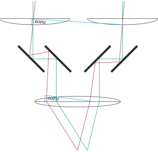
1.4 Homothetic pupil condiion Fizeau’s idea was to place a plate with two holes in the beam path of a telescope. So the telescope be- comes a beam combiner for the two sub-beams. By this procedure the brightness distribution of the source can be determined, but of course there is no extension of the field of view (FoV) nor sensi- tivity. To achieve this goal multiple telescopes must be combined.

It is most important that non-axis sub-beams have no optical-path- differences (OPD), so that the combined beam appears to be from one single telescope (Traub (1986)). This condition is fulfilled when the input and exit pupils of each sub-optic are scaled ver- sions of each other. . . 35 1.5 LINC-NIRVANA PSF for four optical path distances: 0, ¹₃π, ²₃π,π

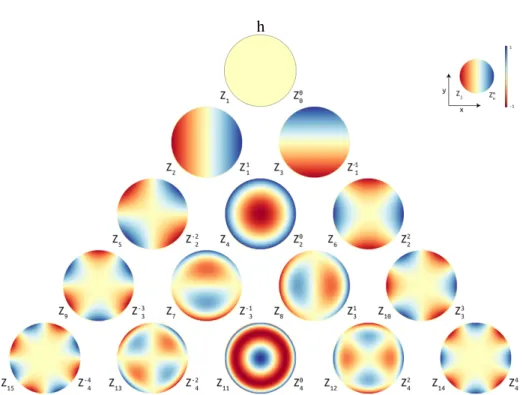
from left to right.(Kürster(2010)) . . . 37 1.6 C²_nprofile for Mt. Graham [Masciadri et al.(2010)] . . . 39 1.7 First 15 Zernike polynomials. Vertically ordered by radial degree

and horizontally ordered by azimuthal degree. [2pem Wikipedia (2015)] . . . 44 1.8 Galactic center, combined in optical, infrared and X-Ray domains

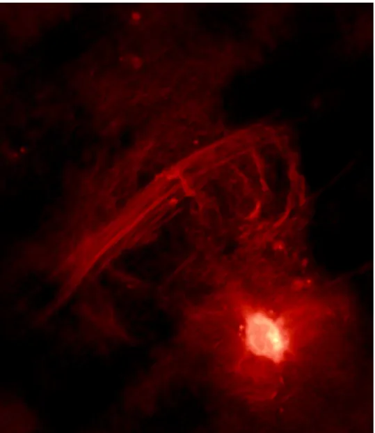
[Image credit toNASA(2018b), "NASA/CXC/SAO"]. . . 49 1.9 Galactic center in radio domain. The bright object in the lower

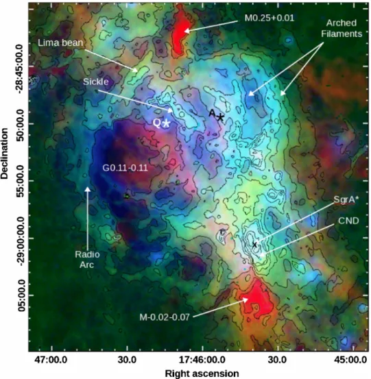
right part is Sgr A*. [Image credit toNASA(2018b), "NASA/CX- C/SAO"]. . . 52 1.10 Galactic center in far-infrared domain in different wavelength: 21.3

µm (blue), 70 µm (green) and 350µm (red). Around the central cavity stretching from 1 to 5 the circumnuclear disk (CND) is vis- ible. [Image credit toEtxaluze et al.(2011)] . . . 54 1.11 Galactic center in infrared domain [Image credit toNASA(2018b),

"NASA/CXC/SAO"] . . . 55 1.12 Galactic center in optical domain [Image credit toNASA(2018b),

"NASA/CXC/SAO"] . . . 56 1.13 Galactic Center in X-ray domain [Image credit toNASA(2018b),

"NASA/CXC/SAO"] . . . 57

1.14 Sagittarius A* in X-ray domain. The image is 15 arcmin across.

[Image credit toNASA(2018b), "NASA/CXC/SAO"] . . . 58 1.15 Parallactic angle The parallactic angleq is a function of the hour

angle and is defines as the angle in the astronomic triangle opposite to the colatitude and between the altitude and (90^◦- declination).

The other two angles are the azimuth and the hour angle. . . 60 1.16 Parallactic angle for various declinations . . . 61 1.17 Parallactic angle for the GC. . . 62 1.18 Altitude variation over the hour angle for various declinations and

the latitude of LBTO (B=32.70^◦). The amplitude of the altitude is bigger for smaller declinations, that means for a object at the equa- tor level the difference between the highest and lowest position is maximal and for a object at north pole level the celestial object ap- pears always on the same altitude. The highest altitude is reached at a declination of about 30^◦. . . 63 1.19 Altitude variation over the hour angle for declination δ = −29^◦

(GC) and latitude B=32.70^◦(LBTO). The maximum altitude is at 28.298^◦where the parallactic angle is 0. . . 64 1.20 Schematic illustration of field rotation: The alt-azimuth mounting

of the LBTO causes the image to rotate in the focal plane. That means the observed image rotates corresponding to equation 1.50 and the image in the focal plane rotates like shown in this figure respectively. . . 65 1.21 Field rotation: The variation ˙qof the field rotation is the first deriva-

tion of the parallactic angleqin equation? and describes how fast the parallactic angle changes and, hereby, how fast the detector must rotate. The first derivation is shown here as graphic for the declinationδ=−29^◦and the latitudeB=32.70^◦ . . . 66 1.22 Large Binocular Telescope (LBT), on Mount Graham in southeast-

ern Arizona at an altitude of 3300 m (LBT(2018)), [Image credit:

Large Binocular Telescope Observatory] . . . 67 1.23 System and sub-system overview of LINC-NIRVANA (Kürster(2010)) 68 1.24 Functional principle of LINC-NIRVANA (Bertram(2007)) . . . . 70

2.1 Software structure: At first in a script file the relevant parameters are set (telescope parameters, stellar field and atmospheric config- uration). In the next steps the simulation loops are performed. The number of loops depends on the simulation time. During the loops in each steps image formation is performed. This input is used to perform the DMs commands, which are used to correct the images.

The next step is to evolve the atmosphere and again format the im- age. After the corresponding number of loops are done, the output algorithms provide the output files, i.a. the long exposure PSF files.

[Tordi et al.(2002)] . . . 75 2.2 Distribution of wind direction and speed: On the left graph the

wind speed in x direction and on the right graph the wind speed in y direction are shown on the y axis. The x-axis represent dif- ferent simulations, that means random distributions for each new calculated atmosphere. The different colours represent the different layers in the atmospheric model. The boxes beneath show the av- erage speed per layer and the corresponding error. The wind speed in both directions is distributed randomly. . . 77 3.1 A grid of 5×5 PSFs were simulated.Each PSF has an edge length of

1360 pixel and is cut to 250 pixel in order to view the non-zero part of the PSF’s due to the fact that these cut out parts are of no interest for further consideration. These crops were made in order to have a better view on the PSFs and has no scientific effect. One can see that the structure of the PSFs are as expected: the PSF which are in the area of the NGS are much more narrow and sharper than in the areas far away from the NGS. This corresponds with the strehlmap shown in figure 3.2 . . . 83 3.2 Strehlmap corresponding to PSFs in figure 3.1: The strehlmap

shape shows a maximum at the right side where the NGS was po- sitioned and slopes in all directions. The parallactic angle for this simulation was 35^◦ and the simulated period was 1 second. The other parameters can be seen in table 2.1. . . 84

3.3 Input pictures: The test input-picture is specifically chosen: all points have the same magnitude and all points distributed homoge- neously so that the effect of the PSF can be estimated for each part of the field of view equally. . . 85

3.4 Input image in 3.3 convolved with each PSF in figure 3.1: These 25 convolved output images show the expected structures. The first convolved image (in the left top) shows only a smudged though rectangular structure. There is a noisy structure in the middle sector and the intensity seems to drop in a rectangular form towards the edges. No single sharp maxima is recognisable. This corresponds with low quality in the strehlmap and the wide and unprecise PSF in figure 3.1. Along the first row towards the fifth convolved im- age, the image quality increases. Although more structures can be seen, the single points from the input image are only vaguely recognisable. The quality of the convolved images in the 2^nd row are already better. Since the 6^th convolved image (1^st convolved image in 2^nd row) is similar to the 5^th, the 10^th convolved image (last image in 2^nd row) already allows to determine all the max- ima from the input image. Also, the diffraction limited structure is recognisable. Especially in the middle the single maxima gets more smudged, but still each maxima is visable. For the 15^th con- volved pictures the best PSF is used. Best means that the PSF is small, sharp and shows the diffraction limited structures. Accord- ingly each maxima is recognisable with its diffraction limited form and all maxima are clearly separated. Since the given PSFs are ax- ially symmetric, the lower halves of the convolved images are very similar to the upper halves. . . 87

3.5 Overall picture stitched together from convolved pictures from fig- ure 3.4: In order to get an overall picture with an edge length of also 250 pixel, each of the 25 convolved pictures are correspond- ingly stitched together. That means that from the first convolved picture in the first row a segment in x-direction from 1 to 50 pixel and in y-direction also 1 to 50 pixel is taken and is put in the seg- ment of the overall picture in x-direction from 1 to 50 and in y from 1 to 50. Then from the second convolved picture in the first row a segment in x-direction from 50 to 100 pixel and in y-direction 1 to 50 pixel is taken and is put in the overall picture in x-direction 50 to 100 pixel and in y-direction 1 to 50 pixel. This is done until from each convolved picture the corresponding part is put in the overall picture. . . 88

3.6 Stitchpoint in the overall picture: Exemplary, the column at the po- sition x=75 was chosen to demonstrate the leaps at the transition point in x-direction 50, 100, 150 and 200. Although the transitions seems to be smooth, the cross section figure 3.7 show the leaps at the transitions points. . . 90

3.7 Transition in column 75 of the overall picture: At the four transi- tion points 50, 100, 150 and 200, leaps are present, that means that the transition are not continuous. Especially at the points 100, 150 and 200 the leaps are very clearly visible. In addition the slope at the points 100 and 200 have different signs and switch from posi- tive to negative at the point 100 and the from negative to positive at the point 200. Although the slope at the point 150 is the same be- fore and after the transition, there is a major gap in the functional value. It is a coincidence that at the point 50 the leap is smaller than at the other transition points.. . . 91

3.8 Smoothed transition in row 75 of the overall picture: After ap- plying the cosine-bell function on the cross section of the overall picture at x=75, it can easily be seen that at the transition points are smoother than before. Both slopes at each transitions show the same value before and after the transition and it is only left a small leap at the point 200. . . 91 3.9 Final overall picture with smoothed transitions: Finally, after ap-

plying the cosine-bell function to all transitions for both x and y direction the final convolved and stitched together picture is shown in figure 3.9. Corresponding to the strehlmap and the 25 single PSF the smoothed final output image shows the expected structure.

On the left side of the image, where the Strehl ratio is very low, the single input points are not recognisable. In the middle part the image quality increases and some structures are shown but the re- sults are not conclusive. In the middle right part, the diffraction limited image of the point can clearly be seen. In contrast to the un-smoothened image in figure 3.5 there are less hard edges and the transition points are no longer recognisable. . . 93 3.10 The principle of the cosine-bell-function: Red line: unprocessed

original input data Blue line: smoothed, cosine-bell-function ap- plied output data Green line: 1^st cosine-function Purple line: 2^nd cosine-function Principle: the algorithm goes from left to right. To evaluate the value at each stepmover a smoothing width ofn, the functional value of the input data (red line) at the pointmis multi- plied with 1^stcosine function at the point m, the value of (m−n)^th value is multiplied with 2^ndcosine-bell functions at the pointm−n and the sum of this both results gives the new output value (blue line) at the point m . . . 94 3.11 Low resolution 10" x 10" detail pictures of the Galactic Centre in

a resolution of 2000 x 2000 pixel . . . 96

3.12 5x5 simulated PSFs with a centered NGS: The 25 PSFs comply with the specification that the NGS is positioned in the centre of the FoV. The central PSF (the 13^th or 3^rd PSF in 3^rd row) shows clearly a diffraction limited structure. The central and the two secondary maxima are clearly distinguishable and the structure is hardly smudged. This observation also applies for the eight di- rectly adjacent PSFs: the diffraction limited structure is also clearly recognisable, whereby the structure is a little more smudged. Also the outer lying PSFs show a central and mostly secondary maxima, but as expected the structures are more smudged. In general, the shown PSFs have a high quality. . . 98

3.13 10" x 10" detail around the Galactic Center in low resolution: The given image show the expected structure: the central part shows detailed structures and the diffraction limited images of the point sources are recognisable. Radial outward going the image quality decreases and although still diffraction limited sources can be seen, these structures are more smeared. . . 99

3.14 10" x 10" detail around the Galactic Centre in higher resolution. . 100

3.15 Convolution with a low resolution picture of the gc (Fig. 3.11) and the PSFs in (3.12): The image quality of the single convolved im- ages is correlated to the PSFs shown in figure 3.12: The image in the centre show detailed structures and single sources are recog- nisable. This good image quality also applies for the eight directly adjacent images: detailed structures are also given, although the structure in the centre starts to smear. This effect of smearing in- creases for the outwards images and instead of single sources the centre structure becomes mashed up. . . 101

3.16 Strehlmap corresponding to PSFs in figure 3.12: The Strehl ratio goes up to 90 % in the middle and falls circular to a value of 20 % to 25 %. The strehlmap is extremely symmetric and of very good quality. It must be considered that atmospherical and instrumental effects hardly cause disturbance while imaging through the central arcsecs with a Strehl ration of about 90 %. Although such a good strehlmap is unrealistic under normal observing conditions, con- volving the corresponding PSFs with the input image helps under- standing the influences of atmospherical and instrumental effects on imaging. . . 102 3.17 10" x 10" detail of the Galactic Centre in high resolution. Fig.

3.14 convolved with Fig. 3.12: Since the PSF quality is extremely good, the convolved image shows in the central part diffraction limited images of single point sources. The output image quality decreases radially outwards. When comparing with the original input picture in 3.14 one can see that although the PSF quality is very good, a lot of details cannot be reconstructed in the convolved output image. . . 103 3.18 Strehlmaps for the 5 different parallactic angles: 1^st image (1^st

image in 1^st row): −30.783^◦ 2^nd image(2^nd image in 1^st row):

−24.698^◦ 3^rd image(3^rd image in 1^st row): 0^◦ 4^th image(1^st im- age in 2^ndrow): 30.783^◦5^thimage(2^ndimage in 2^ndrow): 24.698^◦

. . . 105 3.19 Left: Output picture after de-convolving. Right: Input picture of

Galactic Center in high resolution with science cases (both: 10"

x 10" detail in 2000 x 2000 pixel resolution) The, to be analysed, science cases are marked in figure 4.1 and discussed in chapter 4. Although the single cases are discussed later, one science case (thin dusty filaments, in section 4.3) is marked with a yellow circle in order to show that these structures are still present after the de- convolving process. . . 106

3.20 Image of the convolved Galactic Centre (10" x 10" detail in 2000 x 2000 pixel resolution). The convolved images of the Galactic Cen- tre are shown for 5 different parallactic angles: 1^stimage (1^stimage in 1^strow):−30.783^◦, 2^ndimage(2^ndimage in 1^strow): −24.698^◦, 3^rd image(3^rd image in 1^st row): 0^◦, 4^th image(1^st image in 2^nd row): 30.783^◦, 5^th image(2^nd image in 2^nd row): 24.698^◦. The yellow circles show thin dusty filaments (discussed in section 4.3).

It can be seen that for each parallactic angle these structures are present, although the image quality differs for the parallactic an- gles. In the 2^ndand 5^thimage the structure is clearly recognisable.

The 3^rdimage shows this structure, but is more smudged. In the 1^st and 4^thimage still a maxima is visable, but is hardly discernible as a linear structure. . . 107

4.1 Science Cases, 10" x 10" detail around the Galactic Centre:α, β, γandδ:

Proper motions, GC, II, III and IV: small stellar associations, A and B: Thin dusty filaments, a, b, c, d, e, f, g, h and m: disk embedded sources, k: cometary and asymmetric bow-shock sources. . . 110 4.2 Stripe α . Top: Original Image, Bottem: Re-Convolved Image.

Each image shows a detail of 3.6" x 0.1". . . 111 4.3 StripeβLeft: Original Image, Right: Re-Convolved Image. Each

image shows a detail of 0.1" x 4.1" . . . 113 4.4 Stripeγ Left: Original Image, Right: Re-Convolved Image. Each

image shows a detail of 0.1" x 5,6" . . . 113 4.5 StripeδLeft: Original Image, Right: Re-Convolved Image. Each

image shows a detail of 0.1" x 5.1" . . . 113 4.6 Mean value for ¯y and error∆yin table 4.5 and point coordinates

(red circles) in tab. 4.1 . . . 113

4.7 Measured point with 1σ-gauss-errors of stripesα,β,γandδ. Red represents the original points in the input image. Green represents the measured point in the re-convolved image. One can see that in stripeαthe position in x-direction is reproduced very well, since the y components vary. This can be seen better in figure 4.7a.

For the stripes β, γ and δit is similar, but in these cases the y- components can be reproduced well and the x-components vary. It is important to mention that although in the input image all points are placed in a line (red line), the linearity can not always be deter- mined. The reason therefore is that in very dense regions the placed points are difficult to find. The gaussian fit is performed for a 10 px x 10 px area around the known position of the input points. In cases where multiple sources are in this area, the gaussian function may fit another source and performs the fit accordingly. . . 116

a Stripeα . . . 116

b Stripeβ . . . 116

c Stripeγ . . . 116

d Stripeδ . . . 116

4.8 Small stellar associations. Left top: Original image of GC. Right top: GC. Middle left: GC III. Middle right: GC II, Bottom left: GC IV. Each image shows a detail of 1" x 1". Like one can see the orig- inal picture of the GC is extremely detailed and star clusters can be identified. The GC in the resulting image after de-convolving shows less structures, but the positions of individual sources can still be determined, although the single structures are expatiated.

Since GC III is farthest away from the the guiding stars, the image quality drops as expected. Almost none of the sources can clearly be determined. Due to the fact that both, GC II and GC IV are closest to the guiding stars more details can be seen. Nevertheless, in both cases an allocation of structures to the original sources is hardly possible. One can see that the background noise is reduced in all re-convolved images. Halos which can be seen in the original image of the Galactic Center lack completely in the re-convolved images. . . 119

4.9 Linear structure A. Left: Re-convolved image. Right: Original input image. Each image shows a detail of 0.275" x 0.25". As one can see the linearity of the original filaments are recognisable.

Since the structure A is closer to guiding stars, more points could be resolved. However, the line structure is broken down to seven more or less separate points, such that the linearity is apparent but does not allow the conclusion that these points are coherent. Also, the individual points are wider than the original line structure width.121

4.10 Linear structure B. Left: Re-convolved image. Right: Original input image. Each image shows a detail of 0.1" x 0.3". As one can see the linearity of the original filaments are recognisable. B is in the re-convolved image reconstructed as a narrow and oblong structure with two separate maxima. Also, the two maxima are wider than the original line structure width. . . 122

4.11 Source a: each image shows a detail of 0.225" x 0.225". The right image shows the original input gaussian source. On the left the re-convolved output source is shown. One can see that the re- convolved image is no longer symmetric, and therefore the fitted gaussian function is narrower than in the original input source. The position determination however is accurate. In the re-convolved image also additional points sources are recognisable. Most likely, these additional structures originate in inaccuracy during the de- convolution process. . . 124

4.12 Source b: each image shows a detail of 0.225" x 0.225". The right image shows the original input gaussian source. On the left the re- convolved output source is shown. The re-convolved image is no longer radially symmetrical and shows two maxima. The gaussian fit matches best on the right maxima. In general, the position de- termination is accurate but the symmetric form of the input point source is mostly lost during the convolution and re-convolution process. . . 124

4.13 Source c: each image shows a detail of 0.225" x 0.225". The right image shows the original input gaussian source. On the left the re-convolved output source is shown. Since in the input image additional structures around the source point are given, in the re- convoluted image these structures are missing. In general, the ra- dial symmetric form is given in the output image, although there is no longer a single, centre maxima, but two maxima slightly be- low and above the original maxima of the input image. Above the central structure also small round structure is recognisable. . . 125

4.14 Source d: each image shows a detail of 0.225" x 0.225". The right image shows the original input gaussian source. On the left the re-convolved output source is shown. In the input image, sev- eral structures around the central gaussian source are given. These structures are lost in the re-convolved image, which means that detailed structures cannot be reproduces after re-convolution. Al- though in the output structure the radial symmetric structure of the input source can hardly be seen, the position determination is ac- curate. . . 125

4.15 Source e: each image shows a detail of 0.225" x 0.225". The right image shows the original input gaussian source. On the left the re-convolved output source is shown. The radial symmetric input source is split up into two separate bigger maxima and two minor maxima. The symmetric structure is hereby no longer recognis- able, although the position determination is quite good but varies from the position of the input source.. . . 126

4.16 Source f: each image shows a detail of 0.225" x 0.225". The right image shows the original input gaussian source. On the left, the re-convolved output source is shown. The radial symmetric input source is split up into two separate maxima. The central, more dominant maxima show a radial symmetric structure but is much smaller in diameter. This leads to a smaller 1σ-error of the gaus- sian fit.. . . 126

4.17 Source g: each image shows a detail of 0.225" x 0.225". The right image shows the original input gaussian source. On the left, the re-convolved output source is shown. The radial symmetric input source can be reconstructed in the re-convolved image, since the structure is frayed and smaller in diameter. . . 127

4.18 Source h: each image shows a detail of 0.225" x 0.225". The right image shows the original input gaussian source. On the left, the re-convolved output source is shown. The radial symmetric input source is reconstructed as a more smudged structure, but still a cen- tral maxima is recognisable. Around the central maxima several small structures can be seen. . . 127 4.19 Source k: each image shows a detail of 0.575" x 0.575". The right

image shows the original input gaussian source. On the left the re-convolved output source is shown. The input image shows three comet-shaped sources. Since both the three central maxima and the linearity of the three input source can be reproduced, the comet- shaped characteristics can no longer be seen. This shows that ob- serving comet-shaped structures in the Galactic Centre is still a challenge. . . 128 4.20 Source m: each image shows a detail of 0.225" x 0.225". The right

image shows the original input gaussian source. On the left the re- convolved output source is shown. The radial symmetric structure of the input image is split up into three maxima. The major maxima is positioned slightly below the original position and is narrower than the original one. . . 128 4.21 Position measurement of the three sources k. The red line rep-

resents input sources and the green line the position of the re- convolved sources. Both in the input and the re-convolved image the three sources lay on a line. The error bars for the re-convolved sources are smaller due to the fact that the re-convolved structures are narrower than the original ones.. . . 130 4.22 Sum of disk embed sources a, b, c, d, e, f, g, h and m. Detail of

0.2" x 0.2". . . 131 5.1 Whole FoV divided in 5×5 simulated PSFs with a centred NGS. . 137 5.2 Strehlmap corresponding to PSFs in figure 5.1 . . . 138

5.3 Science Cases, 10" x 10" detail around the Galactic Centre:α, β, γandδ: Proper motions, GC, II, III and IV: small stellar associations, A and B: Thin dusty filaments, a, b, c, d, e, f, g, h and m: disk embedded sources, k: cometary and asymmetric bow-shock sources. . . 139 5.4 Left: Output picture after de-convolving. Right: Input picture of

Galactic Center in high resolution with science cases (both: 10" x 10" detail in 2000 x 2000 pixel resolution). . . 140

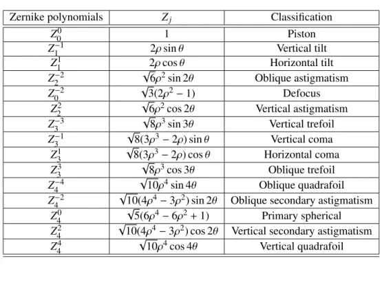
1.1 This table shows the individual Zernike polynomials and their aber- rational meaning. The modes are normalised toR_2π

0

R₁

0 Z²_jρdρdθ=π 45 2.1 This table shows the parameters used to perform the simulations in

chapter 4. . . 80 3.1 Optical reference stars. . . 106 3.2 Simulated parallactic angles. . . 106 4.1 Point coordinates for stripeαincluding 1σ-gauss-error. . . 114 4.2 Point coordinates for stripeβincluding 1σ-gauss-error. . . 114 4.3 Point coordinates for stripeγincluding 1σ-gauss-error. . . 115 4.4 Point coordinates for stripeδincluding 1σ-gauss-error. . . 115 4.5 Mean value and errors of stripesα,β,γandδ. . . 117 4.6 Positions of sources a, b, c, d, e, f, g, h, k and m in the original

image and the re-convolved output, including errors in x and y di- rection. . . 129 4.7 Slope and intersections of the line fits of the three sources k. . . . 130 4.8 Positions of sources a, b, c, d, e, f, g, h, k and m in original image

and re-convolved output including errors in x and y direction. . . . 131 4.9 Mean measuring errors for original and re-constructed image in x-

and y-direction in pixel and milliarcseconds . . . 133

21

AO Adaptive Optic

CCD Charge-Coupled Device (detector) CND Circus Nuclear Disk

DM Deformable Mirror

FoV Field of View

FWHM Full Width Half Maximum

GC Galactic Centre

GWS Groundlayer Wavefront Sensor IDL Interactive Data Language LBT Large Binocular Telescope

LBTO Large Binocular Telescope Observatory LINC LBT INterferometric CAmera

LOST Layer Oriented Simulation Tool mas milli arcsecond

MCAO Multi Conjugate Adaptiv Optics MHWS Mid-High-Layer Wavefront Sensor NGS Natural Guiding Star

NIRVANA Near-IR/Visible Adaptive iNterferometer for Astronomy OPD Optical Path Difference

OTF Optical Transfer Function PSF Point Spread Function Sgr A* Sagittarius A*

SH Shack-Herman (WFS)

SMBH Super Massiv Black Hole

SR Strehl Ratio

VLA Very Large Array 23

WFS Wave Front Sensor

Introduction

In order to extend our understanding of our universe it is crucial to observe it.These observations allow us to create new hypothesis about the evolution of the stars, galaxies and the hole universe and thus our own history. In the other way around once formulated hypothesis also must withstand observations in order to be veri- fied or repudiated. New hypothesis may result in small variations in the measured value, but possibly have a huge impact on our understanding of our universe. So very precise measurements are essential to extend our knowledge about physical laws (we will come to that). A particularly interesting object of study is our Galac- tic Centre. We are about 8 kpc away from the Galactic Centre and electromagnetic waves travel almost the hole distance unimpeded. But only almost, since Earth’s atmosphere disturbs the arriving wavefronts on the last 100 km and causes uneven and non-parallel wavefronts.

We all know this effect from flicking above hot roads or hot air around plane engines as in figure1. The same effect takes place when we watch the stars at night.

As beautiful as the twinkling of the stars may be, this effect reduces the quality at imaging celestial objects significantly .

25

Fig. 1: Flickering hot air around jet engines. [Image credit to NASA (2018a), "NASA Armstrong Flight Research Center"]

Fig. 2: Left: observation without adaptive optics, Right: observation with adaptive optics, [Image credit to GMT (2018), "Giant Magellan Telescope"]

This thesis deals with these disturbances; not only with their cause and effect, but also with the actions to reduce them, namely adaptive optics. Adaptive optics are capable to smooth and to co-phase incoming wavefronts with adjustable mirrors

which adapt to the uneven wavefront. The potential of this technique can be seen in figure2.

In order to investigate these corrective effects, certain constellations are sim- ulated. Although such a simulation has a great number of parameters, the main criteria are

From where is observed?Mount Graham, southeastern Arizona, US With which telescope is observed?The large Binocular Telescope What is observed?The Galactic Centre

Looping back to precise measurements: What do the limitation of atmospher- ical disturbances mean for Earth based observations of celestial objects like the Galactic Centre? In other words: How precisely (with which error) are we able to observe our Milky Way?

Answering this question is the main purpose of this thesis.

Theory

In observational astronomy celestial objects are studied by using telescopes. Since the beginning of modern times, optical telescopes are used to observe the sky. The first type of telescopes were refractors, that gathered optical light waves by curved lenses. In figure 1.1 the schematic of a refractor telescope is shown. The light reflected from the object4)passes through the entry lens1)and is deflected toward the focus point 5). It must be noted that the image in the focus point is upside down. The light passes through the exit lens2)and reaches the eye3). The virtual image6)is what is seen through the exit lens.

Fig. 1.1:Principle structure of a refracting telescope. (Tamás (2018)) 1)Front lens

2)Rear lens 3)Eye

4)Original object 5)Focus point 6)Virtual image

29

Soon after the first refracting telescopes, reflecting telescopes with parabolic mirrors as gathering element were invented. The advantages of reflecting tele- scopes compared to refracting telescopes are the reduction of spherical aberrations and the absence of chromatic aberrations. In Fig. 1.2the schematic of a Newto- nian telescope (a special kind of reflecting telescope) is shown. The electromag- netic wave enters through the entry pointa)and is focused by a concave mirrorb) towards the secondary mirrorc)and finally passed through the exit pointd)

a)

b) C)

d)

Fig. 1.2:Principle structure of a reflecting telescope:

The electromagnetic wave enters through the entry pointa)and is focused by concave mirrorb) towards the plain mirrorc)and finally passed through the exit pointd)(Krishnavedala (2018))

Of certain interest for this work are infrared telescopes. Ground based tele- scopes are limited since water vapour in Earth’s atmosphere absorbs infrared radi- ation. Therefore ground based infrared telescopes are placed in high altitudes and dry weather conditions in order to amplify their performance.

1.1 Astronomical interferometer

Astronomical interferometers are arrays of telescopes which are interconnected by the principle of interferometry to measure fine angular details of electromagnetic sources from outer space. The angular resolution of common earth based tele- scopes are insufficient for a great number of astronomical cases since the angular resolution and sensitivity is limited by the size of the aperture of the telescope. The

growth of the aperture is limited by practical reasons because the technological bar- riers of bigger telescopes are not to be underestimated. Measurements of the po- sitions of cosmic objects with sufficient resolution are of immense importance for further progress in astronomy. More accurate measurements allow identification of objects within various ranges of the electromagnetic spectrum. The precise po- sition and the intrinsic movements of celestial objects but also their movement as- cribable to Earth’s parallax are essential to understand the physics of our universe.

Interferometry offers to overcome the limitation of common telescopes. Based on the area of the array of telescopes spanned of an astronomical interferometers, its angular resolution is comparable to a single telescope of the same diameter.

The resolution of a single telescope depends on the investigated wavelengthλand the diameter D and scales to ^D_λ. The resolution of a two-telescope interferome- ter scales to ^B_λ, where the baseline B is the distance between the two telescopes.

The downsides of astronomical interferometers are that they do not collect as many photons as a single telescope of the same size and the maximum angular size of detectable objects are limited by the minimum gap between two telescopes. The biggest challenge in interferometry is to combine the beams in phase after passing the same optical path through Earth’s atmosphere, the telescopes and finally to the point where both beams are combined. The accuracy must lie within a few tenth of the wavelength of the observed spectrum atλ = 600nm. To achieve this accu- racy the interferometer must be mechanical stable, the detectors need a good time resolution and an adaptiv optic to reduce the effects of atmospherical turbulences.

(Jankov (2010)).

1.1.1 Van Cittert - Zernike theorem

We assume a source S emits monochrome radiation with a frequencyυwhich is detected at the point 1 and 2. We also assume the distancedto bed=(d1+d2)/2.

We can write the electric field as

EA(t)=ASe^−2πiυt (1.1)

whereAS is a complex time-independent amplitude. The electric field is an- tiproportional to the distancedto S as: |E| ∝ 1/d. Radiation emitted at S reaches

Source S Focus plane

1 2

Focus plane

1 2 n Source at infinity

L Θ

d₂ d1

Fig. 1.3: Pictograms for the derivating the van Cittert - Zernike theorem. Left: source S at short distance emitting radiation. Observing points 1 and 2. Right: same setup, but this time the source is moved to a very large distance so that the rays appear parallel.

point 1 with a lag compared to point 2. Therefore, when radiation arrives at point 2 att, the radiations arrives at point 1 att+d1/c. One can write the electric field at point 1 as

E1(t)=

√∆SS

d ASe^{−2πiυ(t+d1/c)} (1.2)

where ∆SS is the surface area of the emitting region S. In equation 1.2 we take √

∆SS since we later will integrate over many non-coherent regions and N non-coherent sources increase the amplitude of the electric field by √

N. Equation 1.2can accordingly be written for the observing point 2. The spacial coherence between the observing points 1 and 2 can be written as

hE^∗₁(t)E2(t)i= 1 T

Z _T

0

∆SS

d² A^∗_SASexp

"

−2πiυ d2−d1

c

!#

dt (1.3)

In the case~r1=~r2the measured flux from S is F= c

4πhE₁^∗(t)E1(t)i= c 4π

∆SS

d² A^∗_SAS (1.4)

For the general case~r1,~r2the arriving rays can be seen as quasi parallel since d1/2 |~r2−~r1| (figure1.3, right). The length L in the right part of figure1.3 is given byL=d1−d2= |~r2−~r1|sinΘ, whereΘis the angle between the normal of the focus plane and the source S. We can rewrite L with the vector~nwhich point from the focus plane towards the source S. We then have

d1−d2=~n·(~r2−~r1) (1.5) With equation1.5we can rewrite equation1.3to

hE₁^∗(t)E2(t)i= ∆SS

d² A^∗_SAS exp

"

−2πiυ ~n·(~r2−~r1) c

!#

. (1.6)

By defining~r ≡ ~r2−~r1 and reducing to a 2-D problem by settingrz = 0 we thus get

~n·(~r2−~r1)≡~n·~r=nxrx+nyry (1.7) and obtain

hE^∗₁(t)E2(t)i= ∆SS

d² A^∗_SASexp

"

−2πiυ nxrx+nyry) c

!#

. (1.8)

Equation1.8applies for a single emitting area S and shows a phase shift of δ φ(rx,ry)=υnxrx+nyry

c (1.9)

for the points 1 and 2. When integrating equation1.8over an entire region, one has to substitute∆S by

dSa =d²dnxdny (1.10)

and get

hE^∗₁(t)E2(t)i= Z

A^∗(nx,ny)A(nx,ny) exp

"

−2πiυ nxrx+nyry) c

!#

dnxdny. (1.11) Equation1.11is a 2-D Fourier integral withrx/λandry/λ. The Fourier trans- formed integrandA^∗(nx,ny)A(nx,ny) is the intensityI(nx,ny).

The Fourier transformed image of the observed source is thus the correlation be- tween the observing points 1 and 2.

1.1.2 Fizeau interferometer

In order to obtain the benefits of multiple telescopes, their beams must be coher- ently combined. At the common focus point, the interferometric signal can be detected. This interferometric pattern is calledfringe. In general there are two possible combination points for the fringes:

Pupil plane (Michelson mode)

In the Michelson mode, the ratio of aperture diameter and separation is not constant. The reason therefore is that the diameter of the combined beams stays the same from the exit point of the telescope to the recombination lens.

The consequence is that the image is not a convolution of the object. The field of view of Michelson interferometers is narrower than for Fizeau inter- ferometers.

Image plane (Fizeau mode)

In the Fizeau mode, the ratio of aperture diameter and separation is constant from the exit point of the telescope and the focus plane. This state is called homothetic pupil condition (see fig. 1.4). The advantage of Fizeau mode compared to Michelson mode is the wider field of view.

The fringe pattern in the point where both beams are combined can be de- scribed:

I =I1+I2+2p

I1I2|γ₁₂|cos 2πP λ −φ

!

, (1.12)

whereI1andI2are the intensities of the fields each telescope observes. It must be noted that equation1.12assumes coherent or at least quasi coherent part fields, which is the case for sources at large distances (van Cittert-Zernike theorem). P is the optical path length difference of each field to the point of interference. |γ₁₂| is the normalized complex degree of spatial coherence. It depends on the bright- ness distribution of the sourceB(α, δ). By measuring the degree of coherence at different points on the image plain, the brightness distribution of the source can be reconstructed. The van Cittert-Zernike theorem states (see section1.1.1):

|F(B(α, δ))=|γ₁₂|. (1.13)

The left side of equation 1.13 states the modulus of the normalized spatial Fourier transformation of the brightness distribution of the plane.

ΔOPD

ΔOPD

Fig. 1.4:Homothetic pupil condiion

Fizeau’s idea was to place a plate with two holes in the beam path of a telescope. So the telescope becomes a beam combiner for the two sub-beams. By this procedure the brightness distribution of the source can be determined, but of course there is no extension of the field of view (FoV) nor sensitivity. To achieve this goal multiple telescopes must be combined. It is most important that non-axis sub-beams have no optical-path-differences (OPD), so that the combined beam appears to be from one single telescope (Traub (1986)). This condition is fulfilled when the input and exit pupils of each sub-optic are scaled versions of each other.

Fizeau’s idea was to place a plate with two holes in the beam path of a tele-

scope. So the telescope becomes a beam combiner for the two sub-beams. By this procedure the brightness distribution of the source can be determined, but of course there is no extension of the FoV nor sensitivity. To achieve this goal multiple tele- scopes must be combined. It is most important that non-axis sub-beams have no optical-path-differences (OPD), so that the combined beam appears to be from one single telescope (Traub (1986)). This condition is fulfilled when the input and exit pupils of each sub-optic are scaled versions of each other. This homothetic pupil condition is illustrated in figure1.4.

1.1.3 Telescope point spread function

Distant stars appear as point sources at the sky. When observing these point sources with telescopes, the result is not a point like image. The reason therefore is diffrac- tion in the telescopes aperture. Atmospherical turbulences and aberration amplify this effect by distorting the image. The diffraction is reciprocally to the size of the aperture: the bigger the aperture is, the smaller is the diffraction. The structure of the diffractions is given by the point spread function (PSF) of the telescope and has the form shown in the fig. 1.5. Both, atmospherical turbulences and aberra- tion, will cause broadening and distorting of the PSF. In absence of atmospherical turbulences and aberration the PSF of the telescope is the diffraction-limited and ideal PSF. The diffraction-limited PSF gives the maximum angular resolution. This is the minimum angular separation of equally bright objects that can be detected under perfect conditions. This is a fundamental limit depending on the observed wavelengthλand the diameter D0 of the telescope and cannot be undercut. The minimum angular resolution is

α_C=1.22 λ

D0 (1.14)

α_C is known as Rayleigh criterion.

1.2 Atmospheric turbulences

The light emitted by astronomical objects travels mostly unimpeded over sev- eral lightyears. The wavefronts of these lights can be considered as perfectly

Figure 3: Monochromatic LINC-NIRVANA PFSs four OPDs of 0, 1/3π, 2/3πandπ(left to right).

5.5 Pixel sampling and field-of-view

The LINC-NIRVANA science detector is a Rockwell HAWAII-2 PACE FPA (see aslo next subsection) with 2048×2048 pixels of size 18µm corresponding to 5.11mas on the sky. Hence the total field-of-view (FoV) is 10.5^′′×10.5^′′. More details on the science detector can be found in AD8.

As one can see from Table 3 that assumes that the interference fringes are aligned with the detector colums (see however Sect. 5.7) the pixel width is not sufficient for optimal sampling of the central fringe in the J-band, effectively leading to a loss in spatial resolution. Only at somewhat longer wavelengths is the sampling criterion (two pixels per FWHM) fulfilled.

Table 3: PSF sampling.

Wavelength FWHM of central fringe Separation of central minima

[pixel] [pixel]

1.1µm (monochromatic) 1.5 (2.0) 3.1 (4.8)

J-band 1.7 3.1

K-band 3.3 5.6

For comparison, values in brackets for the 1.1µm wavelength correspond to a full single-dish 23m telescope.

5.6 Science detector characteristics

The main characteristics of the science detector are summarized in Table 4. Note, however, that full testing of the science detector has not yet commenced at the time of writing this document.

Thererfore, the quoted values are either design values or values provided by the supplier and need to be verified. Read-out-noise values are taken from measurements of the similar HAWAII-2 detectors for LUCIFER-1 and 2. Four different standard read-out modes will be available:

•Double-correlated read

•Line-interlaced read

•Fowler sampling

•Sample up the ramp

The double-correlated read and the line-interlaced read are not read-out noise (RON) optimized and Fig. 1.5: LINC-NIRVANA PSF for four optical path distances: 0, ¹₃π, ²₃π, π from left to right.(Kürster (2010))

plane. These conditions state until the wavefronts reach Earth’s atmosphere. Air at 0^◦C and 1 bar has at optical wavelength a refraction index of approximately n = 1.00029, thus is very close to 1 and nearly perfect. But Earth’s atmosphere is fluctuating regarding temperature, pressure and density. These fluctuations are both temporarily and spatially but always subsonic. It can be assumed to a very high degree that the velocity fields are non divergent. Therefore atmospherical turbulences are caused by solenoidal motions. By traveling through this inhomo- geneous conditions the light respectively its wavefront gets distorted. The fluctua- tions in the atmosphere’s parameters result in variation of the refractive index. So light traveling through the atmosphere in order to reach ground based observatories experiences optical aberration. This again leads to different effects when the radi- ation of a celestial object reach Earth’s surface. On the one hand these distortions cause multiple copies of the stars which are close together. This effect is called speckles. On the other hand they cause slight variations in the appearing brightness of the object, calledscintillation. The latter effect can be observed as twinkling of the stars at night.

The reason for atmospherical turbulences are Wind around the observing spot:

Wind flowing over the telescope dome can cause turbulences.

Wind shear:

Earth’s atmosphere consists of different layers. Each layer can have a dif- ferent horizontal velocity. The gradient of the horizontal velocity can be de- scribed asdvx/dzand if the gradient is big, this can lead to turbulent layers.

In this context theRichardson number Riplays a significant role. If

Ri= g

∆h·(dvx/dz)² (1.15)

with g as gravitational acceleration and∆h as altitude difference between two adjacent atmospherical layers, is1, than turbulences occur.

Convection:

Warm air rises due to lower density. When lower levels of the atmosphere head up convectively instability can occur. Then warmer air bubbles rise in higher altitudes. These bubbles can lead to clouds and some even to thunder storms. In smaller scales these bubbles lead toseeing.

1.2.1 Fluctuation of refraction index

Due to its inhomogeneous conditions Earth’s atmosphere can be described as a tur- bulent medium. The critical parameter here is the refractive index which depends on both temperatureT and pressurepand can be described like in Cox (2015):

n1 'n−1≈7.76·10⁻⁵p

T (1.16)

where phas the unit mbar andT is given in Kelvin. Equation1.16shows that the main reason for the distribution of the refractive index are the changing con- ditions of temperature and pressure within the atmosphere. Note that solenoidal¹ turbulences per se do not influence the observation at all. Only differences in tem- perature and pressure among the different layers initiate fluctuations in the refrac- tion index and herebyseeing.

It is necessary to describe this spacial and temporal fluctuations statistically. Kol- mogorov (1941) gave a very simple description for this distribution. Kinetic energy is introduced into in the turbulent flow at large scalesL0and splits into smaller and smaller spacial scales and finally is converted into head, when the eddies reach a critical scale length ofl0. Within this range, the turbulent flow can be considered as homogenous and isotropic eddies. The boundaries between these eddies have

1Solenoidal means in this context, that the turbulences have no compressional components

smooth transitions in order to prevent discontinuities.

The spacial power spectral densityΦ_n(~k) describes in equation1.17the statistical distribution of the size and the number of these eddies like described in Bertram (2007). An extention to the Kolmogorov model is the Karmen model, which de- scribes the spacial power spectral densityΦ^V_n(~k) as

Φ^V_n(~k)= 0.033C_n²

κ²+κ²₀11/6 ·exp −κ² κ_m²

!

(1.17) where for the he spactial wave numberκ = ^2π_l applies ^2π_L0 ≤ κ ≤ ^2π_l

0. C²_n is the refractive index structure function, which is different for each observatory site. The C_n²profile of Mt. Graham is shown in figure1.6.

152 E. Masciadri et al.

Figure 4. MedianC²_N profile obtained with the complete sample of 43 nights, the summer (April–June) and winter (October–March) time samples. Results are obtained with the standard GS technique. Dotted lines: first and third quartiles.

Figure 5. Left-hand panel: median potential temperature calculated using the ECMWF analyses. Right-hand panel: median wind speed calculated using the composite profile (GS below 2 km, ECMWF analyses above 2 km – see text) in summer (thin style line) and winter (bold style line).

strength of the C

in a precise region of the atmosphere, indeed, de- pends on the thermodynamic stability of the atmosphere in the same region.

6.2 HVR-GS: vertical distribution for h ≤ 1 km

The OT vertical distribution with high resolution (20–30 m) in the first kilometre is obtained with the method called HVR-GS pre-

sented in Egner & Masciadri (2007). The HVR-GR data set is obtained by taking the integral of the C

profiles retrieved from the AC frames and redistributing the energy in the first kilometre according to the detected triplets in the CC frames. Three differ- ent strategies can be used to study the turbulence spatial distri- bution in the boundary layer. The usefulness of each method de- pends on the application one intends to give to the analysis. We study the following.

⃝C 2010 The Authors. Journal compilation^⃝C 2010 RAS, MNRAS404,144–158

by guest on September 6, 2015http://mnras.oxfordjournals.org/Downloaded from

Fig. 1.6:C_n²profile for Mt. Graham [Masciadri et al. (2010)]

It is most important to understand the variation of the refraction index between two spatially separated points in order to handle the wave propagation through the atmosphere. The variance of the refraction indexnbetween two pointsr~0andr~1is

defined as:

Dn(r)=h|n(r~0+r~1)−n(r~0)|i. (1.18) Equation 1.18 is called the refraction index structure function and it can be shown that by assuming Kolmogorov statics it results in:

Dn(r)=C²_n·r^2/3 (1.19)

The variation of the refraction index in the atmosphere causes an immediate perturbation of the wavefront which travels through. The emitted wavefront from the distant astronomical source can be assumed as plane before it passes our at- mosphere. In order to simulate the perturbation of the wavefront we assume a discrete number of atmospheric layers. Furthermore we assume that each atmo- spheric layerihas a constantC²_ni with the altitude zi and the thickness∆z. The vector∆~x represents the separation of two points in a plain perpendicular to the direction of the propagation.ui(x) is the complex optical field in theith layer. The spatial correlation function is given by

Γ(∆~x)=hui(~x)u^∗_i(~x−∆x~ i=exp

"

−1

2DΨ_i(∆~x)

#

(1.20) whereDΨ_i(∆~x) is the phase structure function

DΨi(∆~x)=

* k²

Z _zi+∆zi

zi

dz[n1(~x,z)−n1(~x−∆~x,z)]

!+

(1.21) and k the optical wave number. It can be shown, assuming Kolmogorov statistic and that the thickness of eachith layer is much larger than |∆~x|, that the phase structure function can be written as (Fried (1966))

DΨ_i(∆~x)=2.91k²∆ziC²_ni|∆~x|^5/3. (1.22) Fried (1966) definedr0 as diameter of an area in which the phase error is not more than∼1rad.

r0=0.185









4π² k²P_N

i=1Cn²_i∆zi









3/5

= 0.423k²secγ Z

C²_n(z)dz

!−3/5

.

(1.23)

In order to obtain the same angular resolution when observing an object in long exposure, one would need a telescope with the diameter of r0. The dependency between the Fried parameter and the wavelength is

r0 ∝λ^6/5. (1.24)

This leads to the image size (also known asseeing discorseeing PSF) of α_seeing∝ λ

r0 ∝ 1

λ⁵. (1.25)

Equation 1.25shows that the seeing PSF loses significance compared to the diffraction limited PSF for longer wavelength.

With the Fried parameter follows for the phase structure functionDΨ_i(∆~x)

DΨ_i(∆~x)=6.88 |∆~x| r0

!5/3

(1.26) and for the total spatial correlation functionΓ(∆~x)

Γ(∆~x)=exp









−3.44 |∆~x| r0

!5/3





. (1.27)

Without turbulences then isΓ(∆~x)=1.

1.2.2 Strehl ratio

The obtained image I(~r) in the focus plane contains both the real image of the observed celestrialI0(~r) object and the aberrations caused by atmospherical distur- bances and the telescope. These aberrations can be described by the point spread function (PSF)