Research Collection
Doctoral Thesis
Development of Quantum Applications
Author(s):
Heim, Bettina Publication Date:
2020
Permanent Link:
https://doi.org/10.3929/ethz-b-000468201
Rights / License:
In Copyright - Non-Commercial Use Permitted
This page was generated automatically upon download from the ETH Zurich Research Collection. For more information please consult the Terms of use.
ETH Library
d i s s . e t h n o . 2 7 0 5 3
D E V E L O P M E N T O F Q U A N T U M A P P L I C AT I O N S
A thesis submitted to attain the degree of d o c t o r o f s c i e n c e s of e t h z u r i c h
(Dr. Sc. ETH Zurich)
presented by b e t t i na h e i m M. Sc. ETH Zurich born on 2 July 1989 citizen of Switzerland
accepted on the recommendation of Prof. Dr. M. Troyer, examiner Prof. Dr. R. Renner, co-examiner Prof. Dr. H. Katzgraber, co-examiner
2020
To my husband and family.
A B S T R A C T
The aim of this thesis is to identify practical applications where quantum computing could have an advantage over what is achievable with conventional means of computing, and what advances are needed in order to actualize that potential.
We investigate the possibilities on both quantum annealing devices (analogue quantum computers) as well as on gate-based devices (digital quantum computers).
Quantum annealing devices in particular have grown in size and capabilities over the last decade. While they are natural candidates for providing improved solvers for NP-complete optimization problems, the number of qubits, accuracies and available couplings are still limited and their aptitude has yet to be confirmed. We use Monte Carlo methods and conceive an adaptive annealing schedule to assess the options to leverage them for the construction of satisfiability filters. We furthermore investigate their prospective as heuristic solvers for the traveling salesman problem, and what future enhancements in terms of geometries and couplings would be beneficial for that. Based on our simulations there is no reason to expect any benefits to leveraging analogue quantum computers over state-of-the-art classical methods.
However, we see an implementation of annealing schemes on future digital devices as a promising approach that doesn’t suffer from the same issues that impede performance on analogue devises. To that effect, we construct and implement an efficient quantization of the Metropolis-Hastings algorithm. Opposed to following the common way of quantization à la Szegedy that is usually defined with respect to an oracle, we reformulate the walk to closely mimic the classical algorithm and thus circumvent having to rely on costly quantum arithmetics. Our proposed realization thereby can lead to substantial savings. While theoretical arguments promise a quadratic speedup in the asymptotic limit, we numerically confirm that a polynomial speedup in terms of minimal total time to solution can be achieved for pragmatic use. We explore the prospects of using quantum walks in a heuristic setting and estimate the gate times the would be required to outperform a classical supercomputer.
Finally, we elaborate on the role of programming languages, and how software tools can accelerate the advancement of the field. We discuss unique aspects of quantum programming and the purpose of Q# in particular, and conclude by highlighting what developments are needed for quantum computing to live up to its potential.
iii
Z U S A M M E N FA S S U N G
Das Ziel dieser Dissertation ist es praktische Anwendungen zu identifizieren, bei denen Quantencomputer einen Vorteil gegenüber herkömmlichen Methoden erbrin- gen, sowie welche Fortschritte nötig sind, um dieses Potential umzusetzen.
Wir untersuchen die Möglichkeiten dafür im Bezug auf analoge Quantencomputer sowie digitale. Insbesondere analoge Hardware ist im Laufe des letzten Jahrzehnts grösser und fähiger geworden und ist ein naheliegender Kandidat zur Lösung von NP-kompletten Problemen. Jedoch sind die Anzahl von Qubits, deren Genauigkeit und die verfügbaren Kopplungen limitiert, sodass ihre Eignung erst noch bestä- tigt werden muss. Wir verwenden Monte Carlo Methoden und entwickeln einen adaptiven Prozess um ihre Nützlichkeit für die Konstruktion von SAT-Filtern abzuschätzen. Ebenso evaluieren wir ob sie als besonders gute heuristische Löser für das Rundreiseproblem fungieren können, und welche zukünftigen Entwicklun- gen bezüglich Geometrie und Kopplungen der Machinen dafür vorteilhaft sind.
Basierend auf unseren Simulationen schliessen wir, dass es keinen Grund gibt anzunehmen, dass solche anologe Hardware klassischen Methoden überlegen sind.
Eine Implementierung dieses Prozesses auf digitaler Hardware hingegen könnte vielversprechend sein. Wir entwickeln daher eine effiziente Quantisierung des Metropolis-Hastings Algorithmus die mittels digitalen Quantencomputern einge- setzt werden kann. Im Gegensatz zu einer Quantisierung gemäss Szegedy, welche im Üblichen ein Orakel benutzt, erreichen wir es mit unserer Formulierung kostspie- lige Quanten Arithmetik zu vermeiden. Die präsentierte Umsetzung erweist sich damit als wesentlich kostensparender. Theoretische Argumente basierend auf dem asymptotischen Limit versprechen, dass ein quadratischer Geschwindigkeitsvorteil mittels Quantisierung erreicht werden kann. Wir bestätigen mit einer numerischen Studie eine polinomiale Überlegenheit für die heuristische Anwendung und geben die nötigen Geschwindigkeiten für die Ausführung von Instruktionen an, um einen klassischen Supercomputer zu übertreffen.
Letztendlich diskutieren wir die Rolle von Programmiersprachen und wie geeignete Software die Ausarbeitung von Quantenapplikationen beschleunigen kann. Wir erklären die einzigartigen Aspekte beim Programmieren von Quantencomputern und den Zweck der Sprache Q#. Abschliessend heben wir die Entwicklungen hervor, die stattfinden müssen damit Quantencomputing seinem Potential gerecht wird.
iv
A C K N O W L E D G E M E N T S
I would like to thank my husband Stefan Baumann, without whose support this work would not have been possible. I would like to thank my parents whose unwavering faith in me has always pushed me to be a better person.
I would like to thank Matthias Troyer who not only has been a fantastic mentor but is also a true inspiration.
Furthermore, I would like to thank the collaborators that contributed to the work discussed in this thesis. First and foremost, I would like to thank the co-authors of the papers that served as the basis for this thesis (in alphabetical order): Alan Geller, Andres Paz, Christopher Granade, Daniel Herr, Dave Wecker, David Poulin, Ethan Brown, Guglielmo Mazzola, Jessica Lemieux, John Azariah, Krysta Svore, Mariia Mykhailova, Mario Könz, Marlon Azinovi, Martin Roetteler, Mathias Soeken, Matthias Troyer, Sarah Marshall, and Vadym Kliuchnikov.
Thanks go to Ilia Zintchenko for providing the translation of ak-SAT prob- lem to an Ising spin glass problem, and to Alex Kosenkov, Ilia Zintchenko, and Ethan Brown for providing and supporting thewhiplashframework for easier management of measurement data. I thank Andreas Elsener, Donjan Rodic, Guang Hao Low, Guiseppe Carleo, Guillaume Duclos-Cianci, Jeongwan Haah, José Luis Hablützel Aceijas, Matt Hastings, and Thomas Häner for stimulating discussions. I thank Ali Javadi-Abhari, Julien Ross, Margaret Martonosi, and Peter Selinger for sharing their insights and input on quantum programming languages.
Last but not least, I would like to express my gratitude the work of the people who set up and maintain the spinglass server [1] that was used for the calculation of ground state energies.
v
C O N T E N T S
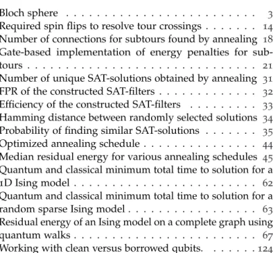
List of Figures ix
List of Tables x
List of Programs xi
1 i n t r o d u c t i o n 1
1.1 Quantum states and qubits . . . 2
1.2 Analogue quantum computing . . . 4
1.3 Digital quantum computing . . . 5
2 t r av e l i n g s a l e s m a n p r o b l e m 10 2.1 Mapping the TSP to an annealing problem . . . 11
2.1.1 Transition probabilities in quantum annealing . . . 11
2.1.2 Encoding as permutation matrix . . . 12
2.1.3 An improved encoding . . . 15
2.2 Numerical results . . . 17
2.3 Digital quantum annealing . . . 20
3 s at f i lt e r s 22 3.1 Set membership problem and filter construction . . . 23
3.2 Quality metrics for filters . . . 25
3.2.1 False positive rate . . . 25
3.2.2 Filter efficiency . . . 26
3.3 Obtaining independent solutions . . . 26
3.3.1 Using annealing . . . 27
3.3.2 Using SAT-solvers . . . 30
3.4 Numerical results . . . 30
3.4.1 Diversity of solutions . . . 31
3.4.2 Quality of solutions . . . 32
3.4.3 Scaling with problem size . . . 37
3.5 Possible improvements . . . 38
4 a n n e a l i n g s c h e d u l e s 39 4.1 Adaptive schedule . . . 39
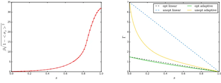
4.2 Calculation of observables . . . 42 vi
c o n t e n t s vii
4.3 Numerical results . . . 43
5 q ua n t u m wa l k s 47 5.1 Szegedy’s quantum walk . . . 48
5.1.1 Eigenvectors and eigenvalues . . . 49
5.1.2 Adiabatic state preparation . . . 50
5.2 Quantization for Metropolis-Hastings algorithm . . . 51
5.2.1 Construction of Szegedy’s walk oracle . . . 53
5.2.2 Alternative walk . . . 54
5.3 Optimization heuristics . . . 59
5.3.1 Algorithm based on the quantum Zeno effect . . . 60
5.3.2 Algorithm based on a unitary walk . . . 61
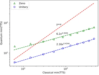
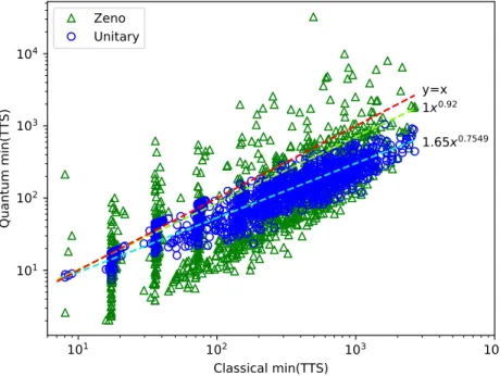
5.4 Numerical results . . . 62
5.5 Irreversible parallel walk . . . 65
6 q ua n t u m p r o g r a m m i n g 69 6.1 Domain-specific concepts . . . 70
6.2 Quantum algorithms . . . 72
6.3 Quantum model of computation . . . 74
6.4 Quantum software frameworks today . . . 76
6.4.1 Use cases . . . 78
6.4.2 Tools . . . 79
6.4.3 Ecosystems . . . 81
7 q ua n t u m p r o g r a m m i n g l a n g ua g e s 84 7.1 Purpose of programming languages . . . 84
7.2 Languages and ecosystems overview . . . 86
7.2.1 Q# . . . 88
7.2.2 OpenQASM and Qiskit . . . 92
7.2.3 Cirq . . . 98
7.2.4 Quipper . . . .102
7.2.5 Scaffold . . . .105
8 d o m a i n-s p e c i f i c l a n g ua g e q# 108 8.1 Design principles . . . .108
8.2 Program structure and execution . . . .109
8.3 Global constructs . . . .113
8.3.1 Type declarations . . . .113
8.3.2 Callable declarations . . . .114
8.3.3 Specialization declarations . . . .116
viii c o n t e n t s
8.4 Statements . . . .121
8.4.1 Quantum memory management . . . .123
8.4.2 Variable declarations and updates . . . .124
8.4.3 Returns and termination . . . .126
8.4.4 Conditional branching . . . .127
8.4.5 Loops and iterations . . . .129
8.4.6 Call statements . . . .130
8.4.7 Other quantum-specific patterns . . . .132
8.5 Expressions . . . .134
8.5.1 Operators, modifiers, and combinators . . . .134
8.5.2 Conditional expressions . . . .140
8.5.3 Partial applications . . . .144
8.5.4 Copy-and-update expressions . . . .145
8.5.5 Item access for user defined types . . . .147
8.5.6 Contextual and omitted expressions . . . .147
8.6 Type system . . . .148
8.6.1 Singleton tuple equivalence . . . .149
8.6.2 Immutability . . . .149
8.6.3 Quantum-specific data types . . . .150
8.6.4 Callables . . . .151
8.6.5 Operation characteristics . . . .152
8.6.6 Type parameterizations . . . .156
8.6.7 Subtyping and variance . . . .159
8.7 Debugging and testing . . . .162
9 i n t o t h e f u t u r e 164
b i b l i o g r a p h y 169
L I S T O F F I G U R E S
Figure1.1 Bloch sphere . . . 3 Figure2.1 Required spin flips to resolve tour crossings . . . 14 Figure2.2 Number of connections for subtours found by annealing 18 Figure2.3 Gate-based implementation of energy penalties for sub- tours . . . 21 Figure3.1 Number of unique SAT-solutions obtained by annealing 31 Figure3.2 FPR of the constructed SAT-filters . . . 32 Figure3.3 Efficiency of the constructed SAT-filters . . . 33 Figure3.4 Hamming distance between randomly selected solutions 34 Figure3.5 Probability of finding similar SAT-solutions . . . 35 Figure4.1 Optimized annealing schedule . . . 44 Figure4.2 Median residual energy for various annealing schedules 45 Figure5.1 Quantum and classical minimum total time to solution for a 1D Ising model . . . 62 Figure5.2 Quantum and classical minimum total time to solution for a random sparse Ising model . . . 63 Figure5.3 Residual energy of an Ising model on a complete graph using quantum walks . . . 67 Figure8.1 Working with clean versus borrowed qubits. . . .124
ix
L I S T O F TA B L E S
Table2.1 Comparison of the number of spin flips required to resolve crossings . . . 15 Table3.1 Average Hamming distance between two 4-SAT solutions found by different solvers. . . 35 Table5.1 Upper bound on the complexity of each component of the walk operator . . . 55 Table5.2 Logical gate times required to outperform a supercom- puter . . . 65 Table7.1 Overview of features of the discussed quantum program- ming languages. . . 87 Table8.1 Overview over available operators in Q#. . . .135 Table8.2 Expression modifiers and combinators in Q#. . . .139
x
L I S T O F P R O G R A M S
Program7.1 Q# code implementing teleportation of an arbitrary quantum state. . . 91 Program7.2 OpenQASM code implementing teleportation of an arbitrary quantum state. . . 94 Program7.3 Python code used to execute OpenQASM programs using Qiskit. . . 95 Program7.4 Qiskit code to generate the OpenQASM circuit for teleporta- tion. . . 96 Program7.5 Cirq code implementing teleportation of an arbitrary quan- tum state. . . .100 Program7.6 Quipper code implementing teleportation of an arbitrary quantum state. . . .103 Program7.7 Haskell code that instantiates the target machine for Pro- gram7.6. . . .104 Program7.8 Scaffold code implementing teleportation of an arbitrary quantum state. . . .106 Program8.1 Q# command line application executing a quantum Fourier transformation. . . .111
xi
1
I N T R O D U C T I O N
Quantum computing exploits quantum phenomena such as superposition and entanglement to realize a form of parallelism that is not available to traditional computing. It offers the potential of significant computational speed-ups in quantum chemistry, materials science, cryptography, and ma- chine learning. Having been a long-standing topic of discussion among scientists, quantum computing has more and more become the focus of public interest as well. Its potential to be more powerful than any conven- tional means of computing and claims that it can revolutionize the way hard optimization problems are solved [2] have piqued the interest of industry.
While there is great hope for the merits that quantum computing could bring, there is also an understanding that any practical application requires algorithmic advances and specialized tools to conquer the challenges unique to working with quantum systems. To build a quantum computer for com- mercially viable applications we need innovations both on the hardware and on the software front. Our effort must include not only a scalable hardware platform, but equally important a sustainable software stack that is capable of supporting its design, control, and the innovations that will eventually lead to a clear advantage of quantum over classical. The idea of a software stack is to build layers of abstraction that encapsulate the required knowledge about different aspects relevant for execution, thus making it available for other layers to build on without having to be aware thereof.
In this thesis we dive into what quantum technology can offer, and what developments are needed to enable large scale quantum computing. We start by looking into some potential applications for quantum annealing devices before looking at the corresponding options and implementations on digital quantum computers. Finally, we muse about how to build a scalable software stack for quantum computing, before detailing the role and purpose of quantum programming languages, and concluding with an outlook into the future.
1
2 i n t r o d u c t i o n
1.1 q ua n t u m s tat e s a n d q u b i t s
Fundamentally, a quantum computer is a machine that stores and processes quantum information. While classical computing models a binary system and employs boolean logic for computation, quantum information is stored in quantum states of matter, and computation is effected by quantum inter- ference. Just as individual binary values are stored in bits, quantum states are stored in quantum bits or qubitsfor short. We will start with a brief introduction of the basic units of quantum information and a description of quantum states.
An idealized quantum system consisting of n logical qubits used for computation is described by a complex state vector inC2n. For instance, the state of a single-qubit system can be written as|ψi=α|0i+β|1i, for some complex numbersαandβ, where|0i..= (10)and|1i..= (01)are vectors forming thecomputational basisfor a single qubit. The componentsαandβ are calledamplitudesand a state of the above form is called asuperposition of the basis states|0iand|1iifα6=06=β.
The amplitudes of a quantum state cannot be observed directly. Instead, measurements are required to extract any information about a quantum state. Measurements are probabilistic and returns onlynbits of information for a quantum system with 2n basis states; measurement selects one output state at random. Evolving under a carefully constructed transformations enables quantum interference to modify the states’ amplitudes and in turn the probability distribution from which one draws the measurement output. Born’s rule provides that the absolute value of the amplitude squared maps to probability space; when measuring the quantum state
|ψi=α|0i+β|1iin the computational basis for example, either state|0ior
|1iis observed with probability|α|2or|β|2, respectively. One may notice that global phaseeiδ does not change these probabilities. In fact, it does not impact any observable properties of the state. This ambiguity is a result of our simplification to represent the state of the quantum system as vector.
More generally, the state of a two-level quantum system would indeed need to be represented not as a vector, but instead as a fulldensity matrix in SU(2). However, quantum computing is merely concerned with pure states, allowing for the simplification of representing the relevant states as a vector rather than a matrix.
For a two-level quantum system (a qubit), the isomorphism between the lie algebra for the group of unitary and hermitian matricesSU(2)and
1.1 q ua n t u m s tat e s a n d q u b i t s 3
ϕ θ
ˆx
ˆy ˆz=|0i
−ˆz=|1i
|ψi
Figure 1.1
Visualization of a single-qubit state via Bloch sphere
the lie algebra of the group of three dimensional rotationsSO(3) allows for an nice geometric representation. A single qubit state is hence often visualized as a point on the surface of the so-calledBloch sphere. Within This geometric representation, a state is defined by spherical coordinatesθ andφ. The angleθdescribes the colatitude with respect to theZ-axis andφ the longitude with respect to theYaxis:|ψi=cos2θ|0i+eiφsinθ2|1i, with 0≤θ≤πand 0≤φ<2π. The pure states that are of interest for quantum computing are on the surface of the Bloch sphere, while points within the sphere correspond to mixed states. The visual interpretation unfortunately breaks down for the multi-qubit case.
The states of a multi-qubit system consisting of unentangled subsystems can be described in terms of the tensor products of valid states for individual subsystems. For instance, a two-qubit state can be constructed as|01i =
|0i ⊗ |1i= (0 1 0 0)t. The set of valid states within the entire computation space is then found by the closure under linear combinations, subject to the consistency requirement that any valid quantum state must be normalized as|hψ|ψi|2=1. The two-qubit state(|00i+|11i)/√
2 is therefore a valid state, despite that there does not exist any pair of single-qubit states that we can assign to each individual qubit. That certain states are impossible to express as a tensor product of the states of individual subsystems implies a particular form of correlation between these subsystems that we refer to as entanglement.
4 i n t r o d u c t i o n
1.2 a na l o g u e q ua n t u m c o m p u t i n g
Some of the earliest physical realizations aspiring to leverage the power of quantum for computing were quantum annealing devices. Such devices compute via (quasi-)adiabatic evolution; the adiabatic theorem [3,4] states that a system that is in an eigenstate of an initial Hamiltonian will remain in the instantaneous eigenstate when the Hamiltonian is changed slowly enough.
In principle, adiabatic quantum computing is polynomially equivalent to gate-based quantum computing [5]. In reality, current implementations in commercial quantum annealing devices [6–8] provide only a limited set of couplings such that only certain kinds of problems can be solved. In particular, unconstrained binary optimization problems (QUBOs) are prime candidates for problems where annealing devices can potentially bring some benefits. QUBO problems can be mapped trivially to an Ising spin glass Hamiltonian with local fields given in Eq. (1.1). Finding the ground state of such Ising spin glass problems in three or more dimensions is an NP-complete problem [9], and many well-known problems from the field of computer science can be mapped to such a description [10,11]. To accommodate hardware restrictions, a QUBO usually needs to be mapped to a more restricted format such as, e.g., the Chimera graph implemented by D-Wave devices [6].
To perform computations, the idea of quantum annealing [12–16] is to start in the easy to prepare ground state of an interacting Hamiltonian and then gradually tune the interaction strength to transition into the ground state of a more complex target Hamiltonian. Within the context of annealing, physical qubits are often referred to asspins, owed in partial due to the fact that currently realizable target Hamiltonians commonly have to take Ising spin glass form
HP=
∑
hs,s0i
Jss0σszσsz0−
∑
s
hsσsz (1.1) where σjzis the Pauli-zmatrices acting on spin j, and the sum goes over all coupling spins. The gradual change of the Hamiltonian is described by two monotonic functions AandB, with A(0) =1,B(0) =0 andA(T) =0, B(T) =1, such that the Hamiltonian at a timetis given by
H(t) =A(t)HD+B(t)HP fort∈[0,T].
A common choice isA(t) =1−t/TandB(t) =t/T. The relation between the interaction or driver Hamiltonian determines the dynamics during
1.3 d i g i ta l q ua n t u m c o m p u t i n g 5
evolution. A usual choice forHDis given by the Hamiltonian of a transverse magnetic field:
HD =−Γ
∑
i
σix.
In analog devices, thermal as well as quantum fluctuations can excite the system, making quantum annealing an approximate solver that will generally find states close to but not necessarily the exact ground state;
crossings or near-crossings in the energy spectrum allow for transitions into excited states (see also Ref. [17]). The size of the spectral gap – if any – determines how slowly the system has to be evolved [18].
Stoquastic Hamiltonian such as the Ising Hamiltonian in a transverse field can be efficiently simulated via quantum Monte Carlo methods. Even though this is true for any stoquastic Hamiltonian, in general it is a highly nontrivial endeavor to identify a suitable set of basis states that would allow to do so. Furthermore, there are recent efforts to realize nonstoquastic Hamiltonians [19]. To simulate quantum annealing on a classical computer, one option is to use path integral Monte Carlo, where the d-dimensional quantum system is mapped onto a classical system in d+1dimensions via a Suzuki-Trotter decomposition, introducing an additional “imaginary time”
dimension [20].
Quantum annealing in spirit is closely related to its classical counterpart;
thermal annealing. Thermal annealing consists of keeping a system in thermal equilibrium with a heat bath while the temperature is slowly decreased to almost zero. If the annealing process is slow enough and the final temperature low enough, the system is forced into its ground state. The idea to simulate this process to solve optimization problems using Markov chain Monte Carlo methods was introduced by Kirkpatrick, Gelatt and Vecchi in1983[21,22]. Whether thermal excitations or quantum fluctuations (tunneling) are more effective to drive the system out of local minima while exploring the problem space depends on the energy landscape or cost function for the problem [23–25].
1.3 d i g i ta l q ua n t u m c o m p u t i n g
Gradually tuning a set of couplings and field strengths to continuously evolve the state of a computation is in contrast to how digital devices perform computations. Digital quantum computers – much like classical computers – operate by implementing a discrete set of instructions. These
6 i n t r o d u c t i o n
are combined to approximate arbitrary transformations of the quantum state during program execution. At the lowest level, quantum algorithms are built from a handful of primitive quantum instructions, just like classical algorithms at lowest level are made of primitives like AND, NOT, and OR gates. Within the context of this these, we will call an instruction that has no effect on the program state other than manipulating the quantum state a quantum gate. A sequence of gates operating on a set of qubits is traditionally called aquantum circuit.
In this section, we will briefly introduce the most basic quantum primi- tives, before elaborating how this historic point of view relates to expressing quantum programs at a similar abstraction level as we are used to in classi- cal software engineering. We will then cover this topic in much more depth in the chapters VI - VIII.
From the perspective of quantum algorithms research, how we think and reason about quantum algorithms is rooted in the mathematical concepts that are at the foundation of quantum computing. Within this model, a computation corresponds to a sequence of mathematical transformations applied to the state vector. These transformations are described by 2n×2n complex unitary matrices or measurements. A unitary matrix is a matrix whose inverse is given by its conjugate transpose, also referred to as its adjoint. For example, a single-qubit state can be transformed from|0ito|1i and back via theXoperator, represented by the unitary matrix
X..= 0 1 1 0
!
. (1.2)
The operatorXcan be seen as a coherent version of a classical NOT gate, mapping an arbitrary superpositionα|0i+β|1itoα|1i+β|0i.
That transformation applied to a particular qubit within a multi-qubit system is obtained by taking the tensor product of X with the identity operator1on the remaining qubits. The effect of applyingXto the second qubit within a three-qubit system, for example, is represented by the unitary operator1⊗X⊗1. We adopt the convention of specifying transformations by their actions on the transformed subsystem and will leave the extension to the entire system implicit. TheXoperator is one of three Pauli operators that together with the identity form a basis for all unitary transformations
1.3 d i g i ta l q ua n t u m c o m p u t i n g 7
on a single qubit. The matrix representations for the other two operatorsY, andZare
Y..= 0 −i i 0
!
, Z..= 1 0 0 −1
!
. (1.3)
Any single-qubit unitary transformation can be expressed as a linear com- bination of these operators. In order to transition from this mathematical perspective to a formulation that is more aligned with how computer programs are commonly expressed, it is convenient to introduce the single- qubit operatorsHandTgiven by
H..= √1 2
1 1
1 −1
!
, and T..= 1 0 0 eiπ/4
!
. (1.4) The Hadamard operatorHis the transformation between the eigenbases ofXandZ, whileT rotates a qubit around theZ-axis. Its squareS..=T2 is the transformation between the X and Y eigenbases. From the given matrix representation we can see that the Hadamard operator H maps
|0i → √1
2(|0i+|1i), and |1i → √1
2(|0i − |1i), whereas up to a global phase, Trotates a qubit around theZ-axis by an angleπ/8.
In order to obtain a finite set of discrete instructions that are universal for arbitrary multi-qubit unitary transformations only one additional in- struction is needed. A common choice is the CNOT operator acting on two qubits. It maps|x,yi → |x,x⊕yi. This operator is represented by the unitary matrix
CNOT..=
1 0 0 0
0 1 0 0
0 0 0 1
0 0 1 0
, (1.5)
and is often referred to as the controlled-NOT, or CX, gate. Conditioned on the state of the first qubit, the transformationXis applied to the second qubit. Such a conditional transformation in a sense can be seen as the “quan- tum version” of a conditional branching, where both branches can execute simultaneously if the condition given by the state of the first qubit being
|1iis a superposition of being satisfied and not satisfied [26]. The concept of this coherent branching can be extended to performing arbitrary multi- qubit transformations conditioned on the state of multiple qubits. Just like
8 i n t r o d u c t i o n
any unitary transformation, suchcontrolledtransformations can be broken down into a sequence of simpler one- and two-qubit transformations [27, 28].
While the ambiguity in the description of quantum state up to a global phase is merely an artifact of our choice to work with the simplified de- scription of the quantum state as a vector instead of the full density matrix, it is worth pointing out that an irrelevant global phase can quickly become local and thus relevant when a gate is executed conditionally on the state of other qubits.
The introduced operatorsT, Hadamard, and CNOT form a universal gate set, i.e., any target unitary transformation can be approximated to arbitrary precision over this gate set. Along with measurement, they can thus be used to express any quantum algorithm [29–31]. The corresponding gate set is of- ten called the Clifford+Tgate set. Examples for which such approximations are needed include rotations around Pauli axes and are common in many quantum algorithms. The corresponding operator isRP(θ) =e−iθP/2, where P∈ {X,Y,Z}denotes one of the Pauli matrices andθ∈[0, 2π)is a rotation angle. For further reading about approximations over the Clifford+Tand other gate sets, we refer to [32–34] and the references cited therein. Besides efficient algorithms for approximation of gates, the Clifford+Tgate set has also several benefits when it comes to circuit optimization and rewriting, see e.g. [35].
When implemented fault-tolerantly, gates can have widely different cost.
In typical fault-tolerant architectures,Tgates are not provided natively but rather have to be created by a special distillation process [36]. This process can create large overheads, depending on the underlying noise level and other architectural parameters. In the Clifford+Tgate set, the cost of aT gate that is several orders of magnitude higher than the cost of H, Z,X, S, andCNOTwhich are all elements of the so-called Clifford group. This motivates to just count the total number ofTgates required by a quantum algorithm implementation and the total circuit T-depth when trying to parallelize as manyTs into stages as possible.
While the Clifford+Tgate set is sufficient to approximate any unitary transformation, it is often convenient to express certain transformations in terms of larger multi-qubit gates. An example for a popular three-qubit gate is the Toffoli gate, also calledCCNOTgate. It maps|x,y,zi → |x,y,xy⊕zi. A possible origin of its popularity lays in the close relation between quan- tum computing and classical reversible computing; any unitary operator by
1.3 d i g i ta l q ua n t u m c o m p u t i n g 9
definition is reversible since for a unitary matrixUit holds thatUU†=I, where † represents the complex conjugate transpose matrix. The mapping defined by the Toffoli gate makes it universal for reversible classical com- puting, since it is capable of implementing any reversible Boolean function given enough zero-initialized ancillary bits.
So far we have covered how to express the reversible parts of a quantum computation. While large parts of a quantum algorithm can be described by unitary transformations, ultimately classical information needs to be extracted for use by non-quantum hardware. Such an extraction is achieved by projecting the state onto the eigenspaces of a unitary operator which yields the corresponding eigenvalue as measurement result. In principle, a quantum state can be projected onto an eigenspace of an arbitrary unitary operator. In practice, only a limited set of measurements are available as hardware instructions, and any other projection is achieved by suitable transformations beforehand. For example, to project a single-qubit state onto the eigenstates of the Xoperator, one would apply the basis trans- formationH, perform the measurement with respect to the computational basis, and reverse the basis switch by applyingHagain. Similarly, to project onto the eigenstates of theYoperator, the basis transformation is given by (SH)† = HS†, with the reversion SH. Despite being non-unitary, projec- tive measurements can be used to manipulate quantum entanglement [37] and are an integral part of a wide class of quantum algorithms. A simple CNOTgate, for example, can be performed using leveraging entanglement, measurements, and single-qubit operations applied conditionally on mea- surement outcomes [38].
A quantum program can be seen as a sequence of primitive instructions such as the elements of the Clifford+T gate set. The sequence is herein generated by a classical algorithm, where the generating algorithm con- tains classical control flow that potentially depends probabilistically on the execution of preceding transformations. Such dependencies arise if the program continuation is conditioned on the outcome of measurement results, and are widely used in particular in the form of repeat-until-success patterns [39–41] and in iterative phase estimation based algorithms [42–44] used in applications such as Hamiltonian simulation [45].
2
T R AV E L I N G S A L E S M A N P R O B L E M
This chapter contains content fromPublication IV.
With progress in quantum technology more sophisticated quantum an- nealing devices are becoming available. Quantum technology is maturing to the point where, for specially selected problems, it can compete with classi- cal computers. Particularly, quantum annealing (QA) devices – performing quantum optimizations by slowly evolving toward a target Hamiltonian – and their potential have been a recent source of controversy. While they offer new possibilities for solving optimization problems, their true poten- tial is still an open question. For a fair assessment of their potential it is necessary to take a close look at the real world problems they strive to solve, and how they can be implemented on a given device. Moreover, how to design such algorithms is becoming increasingly relevant as more and more sophisticated models are starting to become available [46]. As the optimal design of adiabatic algorithms plays an important role in their assessment, we illustrate the aspects and challenges to consider when implementing optimization problems on quantum annealing hardware based on the ex- ample of the traveling salesman problem (TSP).
In this chapter we address factors that determine the performance of quantum annealing algorithms and formulate guidelines for their devel- opment. We discuss the issues that need to be considered when designing specialized quantum hardware and illuminate the challenges and pitfalls of adiabatic quantum computing by examining the case of the traveling salesman problem. We will see that tunneling between local minima can be exponentially suppressed if the quantum dynamics are not carefully tailored to the problem. Furthermore we demonstrate that inequality con- straints, in particular, present a major hurdle for the implementation on analog quantum annealers. Programmable digital quantum annealers can overcome many of these obstacles and can – once large enough quantum computers exist – provide an interesting route to using quantum annealing on a large class of problems.
10
2.1 m a p p i n g t h e t s p t o a n a n n e a l i n g p r o b l e m 11
2.1 m a p p i n g t h e t s p t o a n a n n e a l i n g p r o b l e m
In order to solve an optimization problem by annealing, its solution needs to be encoded into the ground state of the target Hamiltonian. With quan- tum annealing being an approximate solver, it is preferable that in fact all low energy states correspond to solutions that are close to optimal - and to only those. Since the commutation relation between the target and driver Hamiltonian determines the dynamics during evolution, the chosen encod- ing additionally has to permit the use of a simple enough to implement driver that allows for fast transitions between potential solutions.
While in principle it is possible to solve an arbitrary problem on an annealing device, its quantum nature as well as architectural limitations im- pose restrictions on the cost functions and possibly constraining conditions that can be realized. Optimally implementing a given problem thus requires a well chosen mapping onto a suitable target Hamiltonian. The choice of this mapping significantly influences the performance of the algorithm and its scaling with problem size. Whether or not a problem can be solved efficiently by annealing thus depends on both the available hardware and the chosen algorithm.
GivenNcities and distancesdijbetween them, the task of the traveling salesman problem is to find the shortest possible roundtrip that visits each city exactly once. Since current devices provide only local fields and tunable two-site couplings between adjacent qubits, any target Hamiltonian has to correspond to an Ising spin glass.
2.1.1 Transition probabilities in quantum annealing
The ground state of an Ising spin glass can be found by quantum annealing, where the system evolves according to a time dependent Hamiltonian
H(t) = (1− t
T)HD+ t
THPfor 0≤t≤T. (2.1) Consider the transition probability for transitions between two statesψ0 andψ1that each represent a valid tour. Both states are then eigenstates of HP. Assume the system is in a stateψ0at a timet0.T. The probability that
12 t r av e l i n g s a l e s m a n p r o b l e m
the state at a time t0+∆t .T isψ1, if we choose HD = −Γ ∑eσex, ¯h =1, can be approximated by
Pt0(∆t) =
∏
j∈I1
sin2 Γ
T|a(ωj)|
∏
k∈I2
cos2 Γ
T|a(ωk)|+ O(|I1| + 2r) whererN, and
|a(ωk)|2= 4 ω4k
+4t0(t0+∆t) ω2k
sin2(ωk 2 ∆t) +∆t
2
ω2k
−4∆t ω3k sin(ωk
2 ∆t)cos(ωk
2 ∆t) (2.2) The set I1contains all spins whose state differs between the two valid tours,I2all remaining spins. The termsωkare the frequencies belonging to the transition given by flipping spink. While they depend on the state of the surrounding spins, we can neglect this dependency for term up to orderO(|I1|+2r)for r N. We thus make the approximation that the frequencies ωk are independent on the transition path from ψ0 to ψ1 in Eq. (2.2).
In the limitT →∞, const = ∆tT 1, the lowest order contribution to the transition amplitude simplifies to
A(s)(∆t) = Γ∆t T
s shortest
∑
pathsγ
∏
s i=11
E0−E⊥γi (2.3) where sis the minimal path length to transition between the two states.
The energiesEγ⊥i are the eigenvalues of the intermediate states along the transition path, and thus path dependent.
2.1.2 Encoding as permutation matrix
To formulate a TSP as annealing problem, we need to represent every possi- ble valid roundtrip as a spin configuration. The straightforward encoding is to associate each roundtrip with a permutation matrixaik, whereaik=1 if thei-th city is visited at timekof the tour, and zero otherwise [11]. With the mappingaik= (1−σikz)/2 the Hamiltonian can be formulated in terms of quantum spin variables. We then need to ensure that the ground state
2.1 m a p p i n g t h e t s p t o a n a n n e a l i n g p r o b l e m 13
corresponds to the encoding of the shortest roundtrip. Minimizing the tour length given by the Hamiltonian
Hl =
∑
i,j,k
dijaikajk+1forajn+1≡aj1 (2.4) subject to the constraints∑iaik=1∀kand∑kaik=1∀iaccomplishes our goal. These two requirements guarantee that(Mij)is indeed a permutation matrix. They can be implemented by constraint terms
Hc=
∑
i
1−
∑
j
aij
!2
+ 1−
∑
j
aji
!2
, (2.5) which add an energy penalty to states violating them. The ground state of the Hamiltonian
H(perm)P ..= Hl+ηHc
= 1 4
∑
i,j,k
dijσikzσjk+1z +
∑
ik
(d˜i
2 +η(N−3))σikz +η
4
∑
hs,s0i
σszσsz0+const with ˜di ..=
∑
j6=i
1
2(dij+dji)
therefore provides the desired TSP solution. The last sum is over all neigh- boring spins, where we consider two spins to be neighbors, if they either represent the same city or the same time during the tour. The factorηhas to be chosen large enough to ensure that the ground state indeed corresponds to a tour configuration;η≥max{dij/2}.
Such a formulation requires(N−1)2spins, as we can fix cityNto be the last city in the tour, each of which has 2(N−2)neighbors. For an N-city TSP we hence in principle require (N−1)2qubits and 3(N−2)(N−1)2 couplers. Given a typical QA architecture with a small bounded number of couplers per qubit, one will rather needO(N3)qubits.
The quantum driver Hamiltonian HDdetermines the dynamics of the annealing process and should provide an efficient near-adiabatic evolution towards HP without ending up in an excited state. The usual choice is a transverse field term Hx = −Γ ∑i,jσijx, which induces single spin flips.
14 t r av e l i n g s a l e s m a n p r o b l e m
Before contemplating more complex alternatives it is useful to understand the influence of HD on the annealing efficiency.
Figure 2.1
A) A crossing requiring up to 4bN/4csingle spin flips to resolve for a permutation mapping, and only 4 for a symmetric TSP represented by a graph mapping.
B) Worst case forN=18,r=3: Using a permutation mapping, resolving rcrossing requires up to 2 N− d(N−(r−1))/(r+1)esingle spin flips.
Consider the probability to transition between two tours of similar length, as shown inFigure2.1A. This transition can be performed by a so-called 2-opt update [47,48], which is a common and very efficient primitive move in classical heuristics. Using the above mapping this, however, requires to updatem=O(N)variables, since we have to change the order in which half of the cities are visited. The probability to transition between these two tours towards the end of the annealing process is thus – in leading order – proportional to Γ/∆)m, see Eq. (2.3), where∆is the scale associated with the barriers between the two solutions. A simple crossing, as shown in Figure2.1A, is therefore difficult to resolve since the transition probability is exponentially suppressed (in the problem sizeN) compared to classical heuristics that can directly implement a2-opt update.
We thus see that the choices of mappingHPandHDaffect which updates to a configuration are efficiently realized during quantum annealing, and this directly and significantly impacts performance. The above exponential slowdown might be avoided by a better choice of HD orHP. Following the first route we could opt to permute several cities using multi-qubit couplers.
While resolving a crossing may still entailO(N)steps and the exponential suppression remains, this may nevertheless significantly improve transition probabilities by avoiding high energy intermediate configurations that violate constraints. In fact, such kinetics could allow sampling of only viable TSP solutions, which would render the constraints of Eq. (2.5) unnecessary,
2.1 m a p p i n g t h e t s p t o a n a n n e a l i n g p r o b l e m 15
and thereby simplify the energy landscape that needs to be explored [49].
However, the pairwise exchange of all two-city pairs requiresO(N4)four- spin couplers, which is infeasible for all but the smallest problems.
2.1.3 An improved encoding
Independent on the exact dynamics induced by HD, the transition prob- ability declines exponentially with the required number of moves for a transition between two given states. In order to design a mapping that allows for an efficient realization of2-opt (or more generallyk-opt) moves in the quantum annealer, we useN(N−1)spins to represent not the per- mutation, but the the travelled connections between cities, leading to a cost function
Hl0=
∑
i,j
dijaij. (2.6)
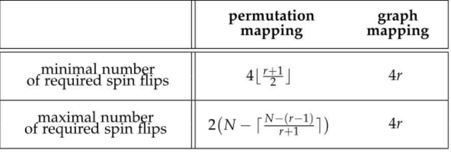
While the required number of moves for a transition between two TSP solutions is approximately the same for both mappings in the asymmetric case, the second map has a clear advantage in the symmetric case. Focusing on symmetric TSPs, a2-opt update using such an encoding as connection graph only requires the flipping ofm=4 spins. More generalk-opt move requires justm=2kflips, independent of the problem size. Such a mapping thus avoids the exponential slowdown of the previous one.
Table2.1gives an overview for the number of single spin flips required to resolvercrossings in both mappings.
permutation
mapping graph
mapping minimal number
of required spin flips 4br+12 c 4r maximal number
of required spin flips 2 N− dN−(r−1)r+1 e 4r Table 2.1
Required number of spin flips to resolvercrossings in the symmetric TSP compared for both mappings
In the case of a symmetric TSP, ie.dij =dji∀i,j, we can associateaij=aji with the undirected edges between citiesiandj, and the number of required
16 t r av e l i n g s a l e s m a n p r o b l e m
spins reduces to 12N(N−1). While the the number of required qubits seems to be comparable atN(N−1)/2, this number can be substantially reduced by truncating the set of considered edges. Along the optimal tour, cities are connected almost exclusively to nearby cities. In fact, the probability of connecting to the l-th farthest city decreases exponentially withl for random problems instances. We can thus truncate the set of considered edges originating at a city to a small number of L closest cities. This substantially reduces the number of required qubits toNL/2=O(N). Implementing the constraints
TSP solutions are subject to the constraint that the set of edges withaij=1 form a valid tour. We expect each city to be connected to exactly two other cities. Closed tours can be enforced by adding a constraint term
Hc0 =
∑
i
2−
∑
j6=i
aij
!2
withaij=aji (2.7)
These constraint terms requireO(NL2)2-qubit couplers, substantially less than the O(N3) terms required for the first mapping. While this term enforces a configuration consisting of closed loops where each city is visited exactly once, it does not in fact enforce that all visited cities belong to the same loop: the tour can break up into disjointsubtoursinstead of one tour connecting all cities. Depending on the specific variant of the TSP this may or may not be desired – one may, for example, want to know if using multiple salesmen is preferred. In that case the target Hamiltonian
HP(graph) =
∑
e
(de
2 +η(N−5))σez+η 4
∑
he,e0i
σezσez0+const
will serve our purpose. The last sum over neighboring spin pairs includes all pairs of spins representing connections with one common start or end point.
However, for randomly generated problems many of the subtours are not particularly interesting. Evaluating100random problems withN=12 and uniformly distributed cities in a2D-plane using CPLEX [50,51] shows that the ground state of75% of the instances splits into subtours and a majority of these subtours contain only three cities. For larger problem sizes, it is likely that here too, we will frequently obtain solutions consisting of a large number of subtours containing only a small number of cities.
2.2 n u m e r i c a l r e s u lt s 17
If we rather want to insist on exactly one closed loop, additional precau- tions will have to be taken. Directly enforcing a single closed tour would requireN-qubit coupling terms and is unrealistic. The standard procedure to avoid such undesired states is to iteratively add terms that penalize thespecificsubtour breakups encountered during the optimization. Given a breakup into, e.g., two sets of cities A and B, we add an inequality constraint of the form
i∈A
∑ ∑
j∈B
aij>0. (2.8)
Unfortunately, such an inequality constraint is hard to implement with two-qubit couplings in an Ising model quantum annealer. Approximating the step function of an inequality by a k-th order polynomial requires implementingO(N2k)k-spin couplings.
Luckily, an evaluation using CPLEX [50] shows that for the ground states of our instances there are very few required connections; around94% of disconnected subtours should have merely two connections with each other and the remaining6% should form four connections. For these a simple quadratic energy penalty
η0 C−
∑
∈A
∑
j∈B
aij
!2
(2.9) with a constant C = 2 to favor two connections or C = 3 to equally favor two and four connections would be sufficient. Such constraint terms increases the number of couplings toO(N2L2), which is still a better scaling than in the original mapping. The algorithm to obtain an estimate for the TSP solution then consists of first annealing the minimally constrained system described by HP =Hl0+ηHc0. If the best solution found splits into subtours, we add additional constraints given in Eq. (2.9) before repeating the annealing. This procedure is repeated until a solution consisting of a single closed tour is found.
2.2 n u m e r i c a l r e s u lt s
We analyzed the effectiveness of this algorithm by numerical simulations on problems withN =8,12 and16 cities. We focus our discussion here on the main results for the caseN=12. We investigated100random TSPs with the cities uniformly distributed on a square.
We start by testing the subtour suppression strategy using the MIQP solver of CPLEX [50]. To avoid any complications due to competing con-
18 t r av e l i n g s a l e s m a n p r o b l e m
straints, we first analyze the performance of the outlined algorithm when choosingC=2 for all iterations. This should enforce the correct behavior for the majority of instances where only two connections between subtours are required. Indeed, after one iteration almost all subtours require merely two connections with only one needing four, and after just two iterations the optimal TSP solution is found for95% of these systems.
number of connections in shortest roundtrip
2 4 6 8 10 12 14 16 18
0 20 40 60 80
probability in %
0 20 40 60 80
0 20 40 60 80
0 20 40 60 80
0 20 40 60 80
0 20 40 60 80
0 20 40 60 80
1
stIteration
2 4 6 8 10 12 0
20 40 60 80 100
2 4 6 8 10 12 14 16 18
MCS 101 102 103 104 105 106 107
4
thIteration
Figure 2.2
Distribution of the number of connections that a subtour found by annealing should have during the first and forth iteration in order to be consistent with the TSP solution. As the state after annealing is generally an excited state, the number of connections can be quite high even for problems where the ground state subtours require only very few connections - even more so the farther we are from the ground state.
The legend denotes the number of Monte Carlo steps (MCS) used for annealing in both panels. The inlay in the “1stIteration” panel shows the distribution for the ground state subtours obtained by an exact solver.
Even though iteratively adding constraints works reasonably well with exact solvers, we found that it fails with heuristic solvers, such as QA, simu- lated QA (SQA), or classical simulated annealing (SA). We show SA results but expect the observations to carry over to SQA and QA. The algorithm succeeds in finding the TSP solution only in very few cases. The reason for this failure is the limited probability of finding the absolute minimum.
Unfortunately, this does not simply translate into a larger number of rep- etitions before the algorithm terminates. Contrary to the ground states, a significant number of the subtours found by annealing should have more
2.2 n u m e r i c a l r e s u lt s 19
than two connections in the TSP solution.
As can be seen inFigure2.2, a poor annealing performance significantly reduces the chance of introducing an appropriate set of constraints. Since enforcing thewrongnumber of connections - that is one inconsistent with the TSP solution - during any one repetition implies that the roundtrip obtained at the end of our algorithm is not of minimal length, the success probability of our algorithm decreases exponentially with the number of iterations.
In an effort to mitigate the detrimental effects resulting from the uncer- tainty about the required number of connections one could pursue several strategies. Adding a penalty function that has multiple minima, e.g., at C=2 andC=4 requiresO(N8)four-spin couplings and is thus not likely to be implementable in the near future. Instead, one might try to choose C=3 in order to equally favors two or four connections, given that an even number of connections is enforced. As the obtained subtours can contain a similar set of cities for several iterations, the ratio η/η0 then needs to be successively increased with each iteration; otherwise the ground state configuration corresponds to broken tours with three connections between subsets of cities. This creates an unfavorable and very rough energy land- scape, where an annealer has barely any chance of finding the ground state. A potential alternative is to use slack variabless1. . .sm,sk∈ {0, 1}, for each subsetAofmcities forming a subtour. One can then implement soft constraints by introducing energy penalties
η0
∑
i∈A
∑
j6∈A
aij−
∑
m k=12ksk 2
+η00 m
k=1
∑
sk−1 2
.
Engineering a suitable energy landscape, however, poses similar challenges, and transitions between solutions with a different number of connections can be heavily suppressed.
We thus conclude that analog quantum annealing devices are unlikely to be of interest as TSP solvers in the near future. The traveling salesman problem demonstrates many important aspects to consider in the design of both adiabatic quantum algorithms and specialized hardware. A so far under appreciated aspect is that quantum dynamics has to be an impor- tant consideration in designing the mapping of an application problem to Ising spin variables. Using transverse fields (or any other local term) for the quantum dynamics incurs an exponential slowdown in the standard
20 t r av e l i n g s a l e s m a n p r o b l e m
faithful mapping of TSP to Ising spins, compared to efficient2-opt updates.
An alternative mapping, which avoids this slowdown and improves the dynamics, comes at the cost of requiring additional constraints to prevent a breakup into subtours. The limitation to quadratic penalty functions in current analog annealing devices constitutes a major problem. In partic- ular the need for inequality constraints presents a major hurdle for the implementation on such devices.
2.3 d i g i ta l q ua n t u m a n n e a l i n g
Virtually all of the above mentioned issues can be remedied by a “digital”
implementation on a gate-model quantum computer that simulates the time evolution of quantum annealing by splitting the propagation into discrete time steps∆t [52,53]. Implementing a constraint ∑imxi = aas a quadratic function(∑mi xi−a)2requiresm2/2 couplers, which results in O(m2)qubits assuming limited connectivity. The same constraint can be implemented in a digital simulation as a phase rotation conditioned on whether the constraint is satisfied or not. Using justO(m)qubits this can be implemented in timeO(logm)(seeFigure2.3a). With this approach the constraint (2.7) requires onlyO(N2)instead ofO(N3)qubits and the cost for the constraint in Eq. (2.8) isO(N2). The scaling of the required number of qubits is thus quadratically improved fromO(N4)toO(N2)(or from O(N2L2)toO(NL)when using a cutoff Lfor the number of neighboring cities considered).
A digital implementation of quantum annealing on a universal quantum computer simulating QA has several other advantages:
• Embedding the program into a specific hardware graph imposes at most linear overhead in runtime, opposed to potentially exponential slowdown of quantum tunneling due embedding into a system with low connectivity in an analog approach.
• The programmability of the digital computer allows efficient imple- mentation of a large class of cost functions and penalty terms; The flexibility offered by a universal digital quantum computer offers more choices of quantum dynamics, including2-opt moves.
• All penalty terms in the cost function can be implemented much more efficiently, reducing the scaling of the number of qubits with problem size.
2.3 d i g i ta l q ua n t u m a n n e a l i n g 21
• The inequality constraint in Eq. (2.8) can now be implemented without heavy approximations.
• A more even energy landscape allows for better annealing perfor- mance.
• Quantum error correction removes calibration errors.
Figure 2.3
a) The left side shows the circuit implementing an energy penalty if a certain subset of cities is disjoint from the rest (inequality constraint in Eq. (2.8)). The qubitsx1. . .xmrepresent all possible connections between the subset and the other cities, the qubitse1..em−2are additional ancilla qubits initialized to|0i(the graphic showsm=6). The 2(m−2)Toffoli gates can be executed inO(logm)time. Open circles denote conditioning on the connectionsxinot being part of the current tour configuration. The unitaryUis a phase gate that implements the propagator corresponding to an energy penaltyη0 during one step of the annealing process by adding a phase exp(−iB(t)η0∆t/¯h)if the qubit is set.
b) As a thought experiment, we could toy with the idea of whether it would theoretically be possible to eliminate all subtours at once. Albeit certainly not of practical value, the circuit on the right illustrates the recursion step for such a circuit. The circuit results in the ancilla qubita1 being set if and only if there is a closed subtour of lengthk+2. The red gates are necessary only to minimize the number of qubits. While this circuit illustrates the principle, using more ancillas allows one to reduce the scaling of the number of gates with system size.
We thus see digital quantum annealers as a promising route to quantum optimization, also because they allow more tailored types of quantum dy- namics to be programmed and – with error correction – solve the calibration and error problems of analog devices. We will further explore this option inChapter5.
3
S AT F I LT E R S
This chapter contains content fromPublication V.
Set membership testing,i.e.determining whether a specific element is a member of a given set in a fast and memory efficient way, is important for many applications, such as database searches. The usage of filters, such as the Bloom filter [54], can give tremendous improvements in terms of resource costs. In2012, Weaver and collaborators introduced a new type of filter, called satisfiability filter [55], which are based on a specific type of Boolean satisfiability problem (SAT), namely randomk-SAT problems, and can achieve a higher efficiency than other popular filters [55–57]. Satisfia- bility filters are a promising type of filters for set membership testing. The creation of a satisfiability filter relies on finding solutions to SAT problems;
to construct a high-quality filter it is necessary to find disparate solutions to hard randomk-SAT problems.
There are many methods which can solve these SAT problems but re- cently with the advent of quantum annealing (QA) a fundamentally dif- ferent method was introduced that can potentially be leveraged for the construction of such filters. A D-Wave Two device has recently been used to construct SAT filters [58] by constucting and solving SAT problems which can be realized with two-qubit couplings. However, the chimera-graph of the D-Wave device does not allow arbitrary connections and thus restricts the types of problems that can be implemented without embedding.
In this chapter, we investigate whether quantum annealing (QA) on an arbitrary connected and completely coherent device can be advantageous for the creation of SAT filters. We compare simulated annealing, simulated quantum annealing and WalkSAT, an open-source SAT solver, in terms of their ability to find suitable k-SAT solutions. Our simulations use an efficient implementation of simulated quantum annealing (SQA), which has been shown to be indicative of the performance of stoquastic Quantum Annealing devices [23,25,59]. We compare the obtained SQA result to those with simulated annealing (SA) and WalkSAT (WS) [60].Section3.3give a brief introduction to SA and SQA related to SAT instances and explains the measurement set-up.
22