Conformal constraints for anomalous dimensions of leading twist operators

(1)

arXiv:1503.04670v1 [hep-th] 16 Mar 2015

Conformal constraints for anomalous dimensions of leading twist operators

A. N. Manashov^a,1,2,3, M. Strohmaier^b,2

1Institut f¨ur Theoretische Physik Universit¨at Hamburg, Luruper Chaussee 149, D-22761 Hamburg, Germany

2Institut f¨ur Theoretische Physik, University of Regensburg, D-93040 Regensburg, Germany

3Department of Theoretical Physics, St.-Petersburg State University, 199034 St.-Petersburg, Russia

Received: date / Accepted: date

Abstract Leading-twist operators have a remarkable property that their divergence vanishes in a free theory. Recently it was suggested that this property can be used for an alternative technique to calculate anomalous dimensions of leading-twist operators and allows one to gain one order in perturbation theory so that, i.e., two-loop anomalous dimensions can be calculated from one-loop Feynman diagrams, etc. In this work we study feasibility of this program on a toy-model example of the ϕ³ theory in six dimensions. Our conclusion is that this approach is valid, although it does not seem to present considerable technical simplifications as com- pared to the standard technique. It does provide one, however, with a very nontrivial check of the calculation as the structure of the contributions is very different.

Keywords conformal invariance·anomalous dimensions

PACS 11.10.Hi·11.25.Db·12.38.Bx

1 Introduction

Calculation of anomalous dimensions of composite operators belongs to the standard tasks of any quantum field theory calculation. For example, in quantum chro- modynamics, anomalous dimensions of leading twist two operators govern the scaling behavior of quark and gluon distributions in hadrons and have to be known with high precision. Nowadays the anomalous dimensions are known at three-loops, see Refs. [1–3] and refer- ences therein. Beyond the two-loop approximation such calculations are feasible only with the help of the ad- vanced methods of computer algebra. Since the calcula-

ae-mail: alexander.manashov@desy.de

be-mail: matthias.strohmaier@ur.de

tions are fully automated finding errors becomes highly nontrivial task and any approach which can provide a check of the final results is very helpful.

Given that the theory depends not only on the coupling constant but also some other parameters such as the dimension of an internal symmetry group, one can organize expansion over these parameters. The best known example of this kind is the 1/N expansion, see Ref. [4] for a review. Agreement between the results obtained in the perturbative and 1/Nexpansions serves as a powerful test for the validity of calculations. However, the calculations in the 1/N expansion are much harder than perturbative calculations: only two RG functions – indices of the basic fields in the nonlinearσ−model and Gross – Neveu model – are available at 1/N³order [5–

7]. In QCD the calculations rarely go beyond the leading order in 1/Nf (whereNf is the number of flavors).

At leading order in 1/Nf the anomalous dimensions of twist two operators were calculated in Refs. [8, 9] but extension of these results to the next order is hardly possible.

A new approach for calculating the anomalous dimensions of leading twist operators was proposed in Refs. [10, 11]. It is still a perturbative approach, however, the contributing diagrams are completely different from those in the standard technique. The approach is based on a remarkable property of leading twist operators: namely, a divergence of such an operator,Oµ1,...µj, vanishes in a free theory [12]

∂^µ¹Oµ1,...µj(x) = 0. (1)

In the interacting theory the r.h.s. of Eq. (1) is non- zero but is proportional to the coupling constant. This identity allows to extract the ℓ−loop contribution to the anomalous dimension of the operatorOµ1,...µj from ℓ−1 loop diagrams only. In particular the one loop

(2)

anomalous dimensions of leading twist operators do not require calculation of loop integrals at all [11, 20].

The method developed in Ref. [11] is adjusted to local operators and relies heavily upon the so-called ”conformal scheme” renormalization [13–15]. In our opinion it is more convenient to stay within the standard MS scheme and the formalism non-local (light-ray) operators technique. This technique proves to be more effective and flexible as we will demonstrate on the example of calculation of two – loop anomalous dimensions in thesu(n) symmetric ϕ³model [16].

The paper is organized as follows. In section 2 we introduce the model and fix notations. In section 3 we recall the light-ray operator technique. Section 4 is de- voted to calculation of the divergence of conformal operator. The details of calculation of two – loop correlators are presented in section 5. Our conclusions are in section 7. In Appendices we explain some technical issues and details of the derivation.

2 Generalities

Thesu(n) symmetricϕ³ model is a scalar field theory in d= 6−2ǫ≡2µdimension with an action

S(ϕ) = Z

d^dx 1

2(∂ϕ^a)²+1

6gM^ǫd^abcϕ^aϕ^bϕ^c

, (2) wherea= 1, . . . , n²−1,

d^abc= 2 trt^a{t^bt^c}, (3)

t^a are the generators of the su(n) algebra normalized in the conventional way, trt^at^b = 1/2. The theory is multiplicatively renormalizable

SR(ϕ, g) =S(ϕ0, g0), (4)

where

ϕ0=Zϕϕ and g0=M^ǫZgg .

Two–loop expressions for the renormalization constants Z1=Z_ϕ² andZ3=ZgZ_ϕ³can be found in Ref. [16]. The β−function of the charge u = g²/(4π)³ and the field anomalous dimensionγϕ are

β(u) =−2ǫu−u²n²−20

2n +O(u³), γϕ(u) =un²−4

12n

1 +un²−100 36n

+O(u³). (5) At the critical pointu∗,β(u∗) = 0,

u∗= 4nǫ/(20−n²) +O(ǫ²) (6)

theory enjoys the scale and conformal invariance.¹ It is well known that in a conformal theory the form of two–point correlation function of conformal operators is fixed up to normalization. In particular, the correlator of the conformal traceless symmetric operators has the form

DO⁽ⁿ⁾_j (x)O^(¯_jⁿ⁾′ (y)E

=δjj^′δ∆j∆j′

CjI_n,¯^j_n(x−y)

((x−y)²)^∆^j . (7) Here j (j^′) is the spin of the operator. The vectors n and ¯n are two light–like vectors, n² = ¯n² = 0, and O⁽ⁿ⁾_j (x) (O^(¯_jⁿ⁾′ (y)) is a contraction of an operator with the vectorn(¯n), for instance

O⁽ⁿ⁾_j (x) =n^µ¹. . . n^µ^jOµ1...µj(x). (8)

∆j and∆j^′ are the scaling dimensions of the operators, Cj is a normalization constant and

In,¯n(x) = (n¯n)−2(nx)(¯nx)

x² . (9)

The scaling dimension of the operator is given by the sum of canonical and anomalous dimensions at a critical point, ∆j = ∆⁽⁰⁾_j +γj, where γj ≡ γj(u∗). For the leading twist operators of spinj,∆⁽⁰⁾_j = 2µ−2 +j.

The anomalous dimension of an operator in MS scheme,γj(u), is a function of a coupling constant only.

It can be restored from its critical value,γj =γj(u∗), provided that the latter is known as a function ofǫ.

The correlation function for the divergence of the conformal operator

∂O⁽ⁿ⁾_j (x)≡j n^µ². . . n^µ^j∂^µ¹Oµ1µ2...µj(x) (10) can be obtained from Eq. (7). Ifxis chosen in the transverse plane, (xn) = (x¯n) = 0, the ratio of the two correlation functions

Tj(u∗) =x²(n¯n)

D∂O⁽ⁿ⁾_j (x)∂O_j^(¯ⁿ⁾(0)E

DO⁽ⁿ⁾_j (x)O_j^(¯ⁿ⁾(0)E (11) is a function of the anomalous dimensionγj only Tj= 2jγj

(2µ−3 +j)(µ−1 +j) µ−2 +j + 2γj

. (12)

This ratio, in full agreement with the result of Ref. [12], vanishes provided thatγj = 0.

1Formally, a nontrivial critical point ford <6 only exists for n = 3,4. However, staying within perturbation theory one can considern as a continuous parameter. In this sense all further results hold for arbitraryn.

(3)

The perturbation series forγj andTj

γj =u∗γ_j⁽¹⁾+u²_∗γ_j⁽²⁾+. . . , Tj =κ_j

u∗T_j⁽¹⁾+u²_∗T_j⁽²⁾+. . .

, (13)

are related to each other. For later convenience we chose the normalization factorκ_j as follows

κ_j =2j(j+ 2)(j+ 3)

j+ 1 . (14)

Substituting the series (13) into Eq. (12) one finds the following relations between the expansion coefficients:

γ_j⁽¹⁾=T_j⁽¹⁾,

γ_j⁽²⁾=T_j⁽²⁾− 2(j+ 1)

(j+ 2)(j+ 3)(T_j⁽¹⁾)² + 2j²+ 5j+ 1

(j+ 1)(j+ 2)(j+ 3)ǫ⁽¹⁾T_j⁽¹⁾, (15) and so on. Hereǫ⁽¹⁾= (n²−20)/4n.

Since the divergence of the conformal operator is proportional to the coupling constant, ∂O⁽ⁿ⁾_j ∼ O(g), the ratio Tj contains a ”kinematical” factor u ∼ g². Thus, in order to determineTj and, hence, the anomalous dimensionγj, withO(u^ℓ) accuracy the corresponding correlation functions have to be calculated at one order inuless. In Ref. [11] one loop anomalous dimensions were reproduced by this method inϕ³ andN = 4 SUSY models. Going beyond the leading order requires an effective technique for calculation of the two–point correlation functions otherwise one gains nothing in comparison with the standard approach.

3 Light-ray vs local operators

The first task is to find a convenient description for local operators. As we will argue the light-ray operator technique [17] is a most suitable one. The light-ray operator²

[O(x;z1, z2)] = [ϕ^a(x+z1n)ϕ^a(x+z2n)] (16) is defined as the generating function for the renormalized local operators

[O(x;z1, z2)]≡X

k,m

z₁^kz^m₂[Okm](x)

= X

k,m,k^′,m^′

z₁^kz₂^mZ_km^k^′^m^′Ok^′m^′(x). (17)

2In order to make presentation more transparent we will consider thesu(n) scalar operator. The operators of other symmetry properties can be easily included into consideration, see Sect.6.

Here [Okm] is the renormalized (in MS scheme) local monomial Okm = ∂₊^kϕ^a(x)∂₊^mϕ^a(x)/k!m! and ∂+ = (n∂x). The sum in Eq. (17) can be replaced by action of some integral operator on the bare operator

[O(x;z)] =ZO(x;z). (18)

Here we introduced a shorthand notationz={z1, z2}.

The integral operatorZ can be written in the form [16]

Zf(z) = Z

dαdβ Z(α, β)f(z₁₂^α, z₂₁^β). (19) The renormalization kernelZ(α, β) is given by a series in 1/ǫand the coupling u. The light-ray operator (17) satisfies the RG equation

M ∂M+β(u)∂u+H(u)

[O(x;z)] = 0, (20) where the evolution kernelHis an integral operator H(u) =−

M d

dMZ

Z⁻¹+ 2γϕ (21)

which encodes all information on the anomalous dimension matrices for local operators.

At the critical pointu=u∗ local operators can be classified according to the representations of the conformal group. An operator with the lowest scaling dimension in the representation is called a conformal operator. The leading twist operator ³, Oj, is uniquely determined by its scaling dimension∆j. The expansion of the light-ray operator (17) over conformal operators and their descendants reads [16]

[O(x;z)] =X

jk

Ψjk(z1, z2)∂₊^kOj(x), (22)

where the coefficientsΨjk(z1, z2) are homogeneous polynomials of degreej+kinz1, z2. These polynomials are eigenfunctions of the evolution kernelH(u∗)

H(u∗)Ψjk(z) =γjΨjk(z), (23) with the corresponding eigenvalues being the anomalous dimensions, γj = γj(u∗). Since the theory enjoys conformal invariance at the critical point u = u∗ the evolution kernel commutes with three generators of the collinear subgroup of conformal group,⁴

[S±,0,H(u∗)] = 0. (24)

3Note, that the operatorOj vanishes identically for oddj.

4Other generators acts on the operators in question trivially.

(4)

The generators, however, deviate from their canonical form (see Appendix Appendix A)

S₋⁽⁰⁾=−∂z1−∂z2, S₀⁽⁰⁾=z1∂z1+z2∂z2+ 2,

S₊⁽⁰⁾=z₁²∂z1+z₂²∂z2+ 2(z1+z2) (25) due to quantum corrections,

S±,0=S_±,0⁽⁰⁾ +∆S±,0. (26) Two of the generators are known to all orders,

∆S−= 0, ∆S0=−ǫ+1

2H(u∗), (27) while corrections to the generator of special conformal transformations can be calculated order by order in perturbation theory [16]. The leading correction is

∆S+= (z1+z2)

−ǫ+1 2H(u∗)

+O(ǫ²). (28) It follows from Eqs. (23), (24) that the operators S±

act as raising (lowering) operators on the set of eigenfunctions Ψjk,

S±Ψjk∼Ψjk±1. (29)

In turnS0 counts conformal spin of the operatorOjk, S0Ψjk=jjkΨjk= 1

2(∆jk+Sjk)Ψjk, (30) where ∆jk = ∆j+k and Sjk are the scaling dimension and spin of the operator, respectively. One derives immediately from (29) that the polynomial Ψjk=0 ac- companying the conformal operator Oj in the expansion (22) is a simple power,Ψjk=0(z1, z2)∼(z1−z2)^j and all other eigenfunctions have the formΨjk(z1, z2)∼ S₊^k(z1−z2)^j.

3.1 Scalar product

Eq. (23) can be considered as a standard quantum mechanical problem for the Hamiltonian H. In order to make this analogy complete one needs to introduce a scalar product on the space of the eigenfunctions. Clearly, such a scalar product has to be adjusted to the sym- metries of the problem. At leading order the answer is given by the standard sl(2) invariant scalar product [18, 19]

(ψ, φ)0= 1 π²

Z Z

|zk|<1

d²z1d²z2(ψ(z1, z2))^†φ(z1, z2). (31)

The integration goes over the unit disks|zk|<1,k= 1,2. The generatorS₀⁽⁰⁾ is a self-adjoint operator with respect to this scalar product and (S⁽⁰⁾₊ )^† =−S₋⁽⁰⁾. We want to find a deformation of the scalar product (31) that keeps these relations for the complete generators, S0=S₀^†andS₊^† =−S−. Let us look for the solution in the form

(ψ, φ)̟= (ψ, ̟φ)0, ̟= 1l +u∗̟⁽¹⁾+. . . , (32) where̟⁽¹⁾is a self-adjoint operator with respect to the scalar product (31). The conjugation conditions for the generators imply

∆S₀⁽¹⁾−(∆S₀⁽¹⁾)^†= [S₀⁽⁰⁾, ̟⁽¹⁾],

∆S₊⁽¹⁾= [S₊⁽⁰⁾, ̟⁽¹⁾]. (33) The one loop corrections to the generators involve the kernelH⁽¹⁾ H(u) =P

ku^kH^(k)

which is given by the following expression

H⁽¹⁾= 2(γ⁽¹⁾_ϕ −λsH⁺). (34) Hereλsis a color factor,λs= (n²−4)/nand

H⁺ψ(z) = Z 1

0

dα Z α¯

0

dβ ψ(z₁₂^α, z₂₁^β). (35) The operator̟⁽¹⁾is completely determined by Eqs. (33).

The explicit expression for̟⁽¹⁾and details of the derivation can be found in Appendix B⁵.

Since the eigenfunctions Ψjk are mutually orthogo- nal w.r.t. the scalar product (32), one can represent the conformal operator as the scalar product of the coefficient function with the light-ray operator

Oj(x) = (z₁₂^j ,[O(x, z)])̟. (36) This representation for the conformal operator is the most convenient one for further analysis. We demonstrate it on the following example. The conformal operator is usually defined as an operator which vanishes under special conformal transformations,Kn¯ =K·n,¯ δK¯nOj(0) = 0. This property becomes transparent in the representation (36) if one takes into account that

δKn¯[O(z)] = 2(n¯n)S+[O(z)],

(we put here [O(z)] = [O(x= 0;z)]) and use that the generatorsS+andS−are conjugate to each other w.r.t.

the scalar product (32),S₊^† =−S−.

5It turns out that the corrections due to̟⁽¹⁾cancel atO(ǫ²) order in the ratio of the correlators (11). So that we do not need this explicit expression for the present purposes.

(5)

4 Divergence of conformal operator

In order to construct the divergence of the conformal operator∂O⁽ⁿ⁾_j , Eq. (10), we calculate first the divergence of the light-ray operator (18)

[∂O(x;z)]≡ ∂

∂x^µ

∂

∂nµ

[O(x;z)]. (37)

Taking then−derivative one cannot, however, keepn²= 0 any longer and has to take into account terms linear in n² which account for the trace subtraction in [O(x;z)].

Taking the corresponding modification into account, see e.g. Refs. [11, 17, 21], one gets for (37)

[∂O(x;z)] = ∂

∂x^µ∇µZϕ^a(x+z1n)ϕ^a(x+z2n) (38) where∇^µ is a differential operator

∇µ= ∂

∂n^µ −1

2(µ−1 +n·∂n)⁻¹n^µ ∂²

∂n². (39) which commutes with the renormalization factorZand acts on the fields directly. After a simple algebra one gets

[∂O(x;z)] = 1

2(S₀^(ǫ)−1)⁻¹Z (

S₊^(ǫ)∂_x²O(x;z)

−L^(ǫ)₂₁ ∂²ϕ^a(x+z1n)ϕ^a(x+z2n)

−L^(ǫ)₁₂ ϕ^a(x+z1n)∂²ϕ^a(x+z2n) )

, (40)

whereS^(ǫ)₀ =S⁽⁰⁾₀ −ǫ,S₊^(ǫ)=S₊⁽⁰⁾−ǫ(z1+z2) and L^(ǫ)₂₁ =∂z2z²₂₁−ǫz21, L^(ǫ)₁₂ =∂z1z²₁₂−ǫz12. (41) Using equations of motion (EOM) one can replace in this expression

∂²ϕ^a(x)7→ 1

2gM^ǫZ3Z₁⁻¹d^abcϕ^b(x)ϕ^c(x). (42) We want to stress here that Eq. (40) holds for arbitrary couplingubut not only at the critical value. Since the l.h.s. of Eq. (40) is a finite (renormalized) operator the r.h.s. can be expressed in terms of renormalized operators with finite coefficients. These operators can be chosen as: the two-particle operator O1 = ∂²O(x;z) and three particle operator

O2=O^(d)(x;w)

=gd^abcϕ^a(x+w1n)ϕ^b(x+w2n)ϕ^c(x+w3n), (43)

wherew={w1, w2, w3}. The operatorsO1andO2mix under renormalization. The mixing matrix (integral operator acting on fields variables) has an lower triangular form

[Ok] =ZkmOm. (44)

Here Z11 = Z is the renormalization constant of the light-ray operator, Eq. (18),Z12= 0,Z21=O(u²) and the elementZ22 is given, at the one loop order, by the sum of two - particles kernels

Z11= 1−u

ǫ λsH⁺₁₂+O(u²), Z22= 1l + u

2ǫ X

i<k λsH^d_ik−λdH_ik⁺

+O(u²), (45) whereλs, λd are color factors

λs= (n²−4)/n , λd= (n²−12)/n . (46) The kernelH_ik⁺ is defined by Eq. (35) andH^d_ik has the form

H₁₂^d f(z1, z2) = Z 1

0

dα αα f(z¯ ₁₂^α, z₁₂^α). (47) The subscriptsik show the arguments the kernel acts on.

Using these results we can rewrite (40) as follows [∂O(x;z)] =1

2(S₀^(ǫ)−1)⁻¹X

k=1,2Ak[Ok(x;z)]. (48) The operatorsAk have the following form:

A1=Z11S₊^(ǫ)Z₁₁⁻¹−M^−ǫA2Z21Z₁₁⁻¹, A2=−1

2M^ǫZ3Z₁⁻¹Z11

L^(ǫ)₁₂S2+L^(ǫ)₂₁S1

Z₂₂⁻¹, (49) where the operatorsS1, S2map functions of three variables to functions of two variables

[S1f](z1, z2) =f(z1, z1, z2),

[S2f](z1, z2) =f(z1, z2, z2). (50) At one loop the operatorsAk take the form

A1=S+(u) +u

λsH⁺−γ_ϕ⁽¹⁾

(z1+z2) +O(u²), A2=−1

2M^ǫ

L12S2+L21S1+

ǫ−uλsH⁺ z12S12

−uz12S12

λsH^d₁₃−λdH⁺₁₃

+O(u²)

. (51) Here S+(u) is given by the expressions (26), (27) for arbitraryu,u∗→u,

S12=S1−S2, Lkm=L^(ǫ7→0)_km

and deriving (51) we made use of the symmetry of the three particle operator Q^(d)(x;w1, w2, w3) under per- mutation ofwvariables.

(6)

Let us stress again that the operators Ak do not contain singular terms forarbitrary u. Using one loop expressions for Z factors, Eq. (45), it can be checked that all pole terms cancel at orderO(u). In particular Z3Z₁⁻¹Z11

L12S2+L21S1

Z₂₂⁻¹=

=L12S2+L21S1+O(u²). (52) Starting from the representation (36) for the conformal operator, we get for its divergence

∂Oj(x) = (z₁₂^j ,[∂O(x;z)])̟. (53) Making use of Eqs. (48) – (51) one finds that the divergence ∂Oj(x) is given by the sum of two–particle and three–particle (renormalized) operators

∂Oj(x) = 1 2(j+ 1−ǫ)

R⁽²⁾_j (x) +R⁽³⁾_j (x)

. (54)

The prefactor on the r.h.s of Eq. (54) is the eigenvalue of the operator (S₀^(ǫ)−1)⁻¹ on the function z^j₁₂. The two–particle termR⁽²⁾_j has the form

R⁽²⁾_j (x) =γj z₁₂^j ,(z1+z2)[O1(x;z)]

+O(u²_∗). (55) We recall that γj =γj(u∗) and O1(x;z) = ∂²O(x;z).

Let us note that the term ∼S+ in the expression for A1, Eq. (51), vanishes inside the scalar product since (z₁₂^j , S+. . .) = −(S−z^j₁₂, . . .) = 0. In turn, the expression for the three–particle contribution can be written as follows

R⁽³⁾_j (x) =R^(3,0)_j (x) +R^(3,1)_j (x) +O(ǫ²), (56) where

R^(3,0)_j (x) =−M^ǫ(z^j₁₂, L21S1[O2(x;z)]

̟, R^(3,1)_j (x) =−M^ǫ(z^j₁₂, z12S1Xj[O2(x;z)]

̟ (57)

and the operatorXj has the form

Xj=ǫ−γϕ+γj/2−u∗ λsH^d₁₃−λdH⁺₁₃

. (58)

This expression follows immediately from (51) if one takes into account that spin j is even and A2 is symmetric under interchangez1↔z2.

It is clear from (55) that the expansion of two particle termR⁽²⁾_j over conformal operators does not contain the operator of spinj,

R⁽²⁾_j ∼∂²

j−2

X

m=0

cm∂₊^j−m−2Om(x)

!

. (59)

Taking into account that hOj(x)Ok(0)i= 0 for k < j one derives that hR⁽²⁾_j (x)∂Oj(0)i = 0. This, in virtue

z2

z1

w2

w1

z2

z1

w2

w1

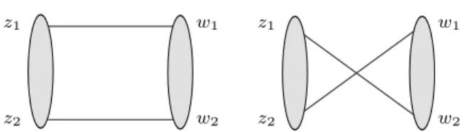
Fig. 1 The leading order diagrams for the correlator of two conformal operators,hO⁽ⁿ⁾_j (x)O^{( ¯}_jⁿ⁾(0)i.

of Eq. (54), results in the following relation for the correlators

hR⁽²⁾_j (x)R⁽²⁾_j (0)i=−hR⁽²⁾_j (x)R⁽³⁾_j (0)i. (60) It can be shown that in the correlatorh∂Oj(x)∂Oj(0)i one can replace (54) by a simpler expression

∂Oj(x) = 1 2(j+ 1)

R⁽²⁾_j (x) +R^(3,0)_j (x)

. (61)

The omitted terms

∆X = ǫ j+ 1

R^(3,1)_j (x) + 1

j+ 1R^(3,0)_j (x)

+O(ǫ²) give rise to the correction of orderO(ǫ³). In order to ver- ify this it is sufficient to notice that∆X can be rewritten in the form (z₁₂^j , F S−z12[O2(x;z)]

̟, where F is some operator whose explicit expression is not relevant.

Inside the correlator the generatorS− acts, finally, on the functionz₁₂^j nullifying it.

Thus in order to find the anomalous dimension γj

at orderO(ǫ²) one has to calculate the three correlators hOjOji, hR⁽²⁾_j R^(3,0)_j i, hR^(3,0)_j R^(3,0)_j i at one loop order. We will do it in the next section.

Finally, we note that forj= 2 the r.h.s. of Eq. (54) has to vanish identically since the operatorOµν is, up to EOM terms, the energy-momentum tensor.The two particle termR⁽²⁾_j is proportional to the anomalous di- mensionγjand therefore vanishes forj= 2. In order to check it forR⁽³⁾_j , it is sufficient to take into account that only the linear term in the expansion of three particle operator

O2(x;w)∼(w1+w2+w3)·d^abc∂+ϕ^a(x)ϕ^b(x)ϕ^c(x)

=

S₊^(1,1,1)·1

d^abc∂+ϕ^a(x)ϕ^b(x)ϕ^c(x) contributes to (56) forj = 2. After simple algebra one finds thatR⁽³⁾_j=2=O(ǫ²).

(7)

z2

z1

w2

w1

z2

z1

w1

w2

Fig. 2 The LO diagrams for the correlator of divergence of conformal operators,h∂O⁽ⁿ⁾_j (x)∂O^{( ¯}_jⁿ⁾(0)i.

5 Correlators

5.1 LO correlators

In order to give a glimpse of the technique we start with calculation of the necessary correlators at leading order.

The correlator hO_j⁽ⁿ⁾(x)O^(¯_jⁿ⁾(0)i is given by the sum of two diagrams, shown schematically in Fig. 1. They are given by the product of the propagators and give rise to identical contributions to the correlation function. Assuming that xis chosen in a transverse plane, (x, n) = (x,n) = 0, one represents the propagator as¯ D(x+z1n−w¯1n) =¯ D(x)(1−z1w¯1r)^−(µ−1), (62) wherer= 2(n¯n)/x² and

D(x) =Γ(µ−1)/(4π^µ(x²)^µ−1). (63) At leading order one replaces µ−1 7→ 2 so that the second factor in (62) is nothing else as the reproducing kernel,Ks=1(z1, w1r), corresponding to the spins= 1, see Eq. (A.5). Therefore starting from Eq. (36) one gets for the correlator

hO⁽ⁿ⁾_j (x)O^(¯_jⁿ⁾(0)i= 2ξD²(x)(z₁₂^j |

2

Y

k=1

K1(zk, wkr)|w^j₁₂)

= 2ξD²(x)r^j||w^j₁₂||²₁₁, (64) whereξ=n²−1 is the isotopic factor, the scalar products correspond to the conformal spin s = 1 and we take into account the property of the reproducing kernel (A.6). The norm of w₁₂^j is given by the following expression

||w^j₁₂||²_s₁_s₂ =j!

2

Y

k=1

Γ(2sk) Γ(j+ 2sk)

Γ(2j+ 2(s1+s2)−1) Γ(j+ 2(s1+s2)−1) . The diagrams for the correlatorh∂O⁽ⁿ⁾_j (x)∂O_j^(¯ⁿ⁾(0)i are shown in Fig. 2. On the leftmost diagram the points z1nand ¯w¯nare connected by two propagators

D²(x+z1n−w¯1¯n) =D²(x)(1−z1w¯1r)^−2(µ−1)

=D²(x)Ks=2(z1, w1r). (65)

Since∂O⁽ⁿ⁾_j ∼(z₁₂^j , L21[O(x, z1, z1, z2)])11, see Eq. (57), thez−scalar product has the form

(z^j₁₂, L21K2(z1, w1r)K1(z2, w2r))11. (66) The spins of the reproducing kernels and spins of the scalar product are in discord with each other. However, the operator L21 = ∂2z²₂₁ removes this mismatch. It intertwines the representations,

L21D⁺₂ ⊗D⁺₁ =D⁺₁ ⊗D⁺₁L21

and it can be easily shown, see e.g. Ref. [20], that (z^j₁₂, L21Φ(z1, z2))11=−aj(z₁₂^j−1, Φ(z1, z2))21, (67) where

aj= (j+ 1)||z^j₁₂||²₁₁/||z₁₂^j−1||²₂₁= j(j+ 2)(j+ 3)

6 . (68)

Thus the scalar product (66) takes the form

−aj(z₁₂^j−1,K2(z1, w1r)K1(z2, w2r))21=−aj(rw¯12)^j−1. (69) Restoring all color and symmetry factors one gets for the first diagram

−1

2ξλsg²D³(x)aj/(j+ 1)²r^j−1(L21w¯₁₂^j−1, w^j₁₂)11=

= 1

2ξλsg²D³(x)aj/(j+ 1)r^j−1||w^j₁₂||²₁₁. (70) The calculation of the second diagram goes along the same line. One can combine propagators attached to the pointz1using the Feynman’s trick to get (z^j₁₂, L21K2(z1, w1r)K2(z1, w2r)K1(z2, w1r))11=

= 6(−1)^jaj(rw¯12)^j−1

(j+ 1)(j+ 2) . (71) Finally, taking into account that second diagram en- ters with symmetry factor 2 one gets, in full agreement with (11),

Tj(u∗) =u∗κ_jγ_j⁽¹⁾+O(u²_∗), (72) where the one–loop anomalous dimension is, see Eq. (34), γ_j⁽¹⁾=λs

1 6

(j−2)(j+ 5)

(j+ 1)(j+ 2). (73)

Thus the diagrams are easily calculated provided that the spins of the reproducing kernels match that of the scalar product. We will show that this scheme can be extended to loop diagrams as well.

(8)

z2

z1

w2

w1

=⇒ z2

z1

w2

w1

=⇒

z^α₁₂ z1

w^β₁₂ w1

µ−1−δ µ−1−δ A

µ−1 +δ µ−1 +δ

µ−1

2−3δ 2−3δ B

1

1−

δ 1−δ

1

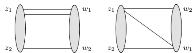
3−3ǫ C Fig. 3 NLO correction to the correlator of conformal operatorshO⁽ⁿ⁾_j (x)O^{( ¯}_jⁿ⁾(0)i. The parameterδ=ǫ/2.

5.2 NLO correlators

First, it is easy to see that the corrections due to modification of the scalar product cancel out in the ratio of correlators. Indeed, these corrections only influence the norm

||w₁₂^j ||²₁₁7→ ||w₁₂^j ||²_̟= (w₁₂^j ,(1 +̟⁽¹⁾)w^j₁₂)11. entering the tree level expressions, Eqs. (64), (70), etc., which cancels out in the ratio of correlators, Tj, irre- spectively of the explicit form of ̟. This cancellation is expected. Indeed, the problem can be reformulated as a standard quantum mechanical problem for a cer- tain Hamiltonian. A modification of the scalar product produces corrections to the eigenstates (conformal operator). However, the energy shift at the leading order, δE_ψ⁽¹⁾ = hψ⁽⁰⁾|V|ψ⁽⁰⁾i, is not sensitive to such corrections.

The calculation of hR⁽²⁾_j R^(3,0)_j i is a bit more in- volved but straightforward. The corresponding contribution toT_j⁽²⁾ reads

T_j^(2→3)=−1

2(γ_j⁽¹⁾)² (j−1)(j²+ 4j+ 9)

(j+ 1)(j+ 2)(j+ 3)(j+ 5). (74) It is convenient to split one loop corrections to the cor- relatorshOjOjiandhR^(3,0)_j R^(3,0)_j iinto two groups

– Self-energy insertions to the propagators.

– All other loop diagrams

Taking into account the self-energy correction to the propagators is equivalent to the calculation of the tree–

level diagrams with the exact (critical) propagator Dc(x) =A(u∗)/(x²)^∆^ϕ, (75) where∆ϕ=µ−1 +γϕis the critical dimension of the basic field and the residue A(u∗) is

A(u∗) = Γ(µ−1) 4π^µM^2γ^ϕ

1−u∗λs

5

36+O(u²_∗)

, (76)

where M² =πM²e^γ^E. For the first diagram in Fig. 1 one gets

D²c(x)r^j (z₁₂^j |Ks(z1, w1)Ks(z2, w2)|w^j₁₂)(11),(11), (77)

wheres=∆ϕ/2 = 1−(ǫ−γϕ)/2, the subscripts indicate the conformal spins of thez andwscalar products, respectively. The reproducing kernels in (77) correspond to spins which does not match the spins of the scalar product. However, it is easy to see that, due to symmetry, the scalar product with modified spins

(z^j₁₂|Ks(z1, w1)Ks(z2, w2)|w₁₂^j )_(s^δ₊_,s^δ₊_),(s^δ

−,s^δ₋), (78)

wheres^δ_± = 1±δis equal to that in (77) up to terms of orderδ². Therefore, choosings^δ₋=s, (δ= (ǫ−γϕ)/2), and evaluating thew−product in (78) one gets for (77) D_c²(x)r^j||z^j₁₂||²_sδ

+,s^δ₊+O(u²_∗). (79)

The calculation of the diagrams in Fig. 2 goes along the same lines. Finally, the contribution to the ratio of correlators Tj from the leading order diagrams and self-energy diagrams can be written in the form (up to O(ǫ²) terms)

T_j^SE= 2u∗λs

κ_j

1 +u∗

2

λd−7 9λs

||z^j−1₁₂ ||²_2sδ +,s^δ₊

||z₁₂^j ||²_sδ +,s^δ₊

×

1−2Γ(4s^δ₋)(Γ(j−1 + 2s^δ₋) Γ(2s^δ₋)Γ(j−1 + 4s^δ₋)

. (80)

Expanding (80) we find for the corresponding contribution to the coefficientT_j⁽²⁾

T_j^SE=γ_j⁽¹⁾ (1

2

λd−7 9λs

+ 2δ

"

S2j+2−Sj+3−Sj+2 3

4j²+ 14j+ 9 (j+ 2)(j+ 3)

#)

− 4λsδ (j+ 1)(j+ 2)

Sj+2−(2j+ 1)(4j+ 7) 3(j+ 1)(j+ 2)

, (81) whereSj =Pj

k=11/kand δ= 1

4

−λd+1 3λs

. (82)

We recall that γ_j⁽¹⁾ is the one loop anomalous dimension, Eq. (73).

(9)

5.3 Loop diagrams

All loop diagrams can be calculated quite easily with the help of several simple tricks. Several examples are given below. Let us start with a correction to the correlator of two conformal operators. The corresponding contribution has the form

C(ǫ) = 2 (z₁₂^j |H(x;z, w)|w^j₁₂)(11),(11), (83) where the kernelH(x;z;w) is given by the left diagram shown in Fig. 3 with the parameterδ→0. We need to findC(ǫ) up to termsO(ǫ⁰) ,C(ǫ) = ¹_ǫ(c0+ǫc1+. . .). To this end we proceed as follows. We modify the indices as shown in Fig. 3. This modification does not change the pole structure (see discussion in Ref. [26]) and, due to the symmetryC(ǫ, δ) =C(ǫ,−δ), one concludes that C(ǫ, δ) =1

ǫ(c0+ǫc1+c2δ²+. . .). (84) The choice δ = ǫ/2 results in the uniqueness of the upper integration vertex and at the same time does not affect first two terms in (84). Using the star–triangle relation for the upper vertex one gets the diagram B in Fig. 3. Using Feynman formula for the left (right) propagators attached to the integration vertex one can perform the last integral that results in the diagramC in Fig. 3.

This diagram, up to a x−dependent factor, has the form

K¹

2(z1, w1) Z 1

0

dαdβ(¯αβ)¯ ^−δ(αβ)^1−3δK³

2−3δ(z^α₁₂, w^β₁₂). (85) On the next step we want to get rid of the paramet- ric integrals. To this end we use the properties of the reproducing kernel (A.6) and represent

Ks−δ(z₁₂^α, w^β₁₂) = Z

d²ξ^′µs(ξ^′)Ks(z^α₁₂, ξ^′) Z

d²ξ µs(ξ)Ks−δ(ξ^′, ξ)Ks(ξ, w^β₁₂)

= Z

d²ξ µs+δ(ξ)Ks(z^α₁₂, ξ)Ks(ξ, w^β₁₂) +O(δ²), (86) wheres= 3/2−2δand we used the relation (A.7). Using this expression one can carry out the integrals overα, β in (85). The resulting expression forH(x;z, w) (up to a prefactor) takes the form of “sl(2)” diagram shown in Fig. 4.

Now we need to calculate the scalar product (83) with the kernel H(x;z, w) given by the diagram on Fig. 4. The scalar product is a function of indices of left (right) propagators and conformal spins of z (w)

z2

z1

w2

w1

α α

β β

γ

Fig. 4 The “sl(2)” diagram: an arrow line fromwtozwith indexαstands for the propagator (1−zw)¯ ⁻^α. The indices have the following values: α = 2−3ǫ/2, β = 1−ǫ/2 and γ= 1. The black circle denote an integration vertex with the sl(2) invariant measureµs+δ,s+δ= 3/2−ǫ/4.

scalar products,S(a, b, s1, s2|a^′, b^′, s^′₁, s^′₂).We need this function up toO(ǫ) terms for a=a^′ =α, b =b^′ =β and si = s^′_i = 1. As was explained in the previous section the integral with measureµs can be evaluated easily provided that the sum of the indices of propagators coming from this vertex is equal to 2s. Taking this into account one finds that the scalar product with shifted indices

S(α+δ, β+δ,1 + 2δ,1 + 4δ|α−δ, β−δ,1−2δ,1−4δ) can be straightforwardly calculated to

S(ǫ) = j!Γ(3−ǫ)

Γ(j+ 3−ǫ)||z^j₁₂||²₁₊1

2ǫ,1+ǫ (87)

and in the same time it differs from the scalar product in question by terms of orderO(ǫ²) only.

Restoring all factors one gets forC(ǫ) C(ǫ) =u∗λs(n²−1)D²(x)(x²M²)^ǫr^j2 +ǫ

ǫ S(ǫ). (88) Since the ratio (11) does not depend onx, it is convenient to put x²M² = 1. Finally, subtracting the coun- terterms

∆C(ǫ) =−1

ǫ4u∗λs(n²−1)D²(x)r^j||z₁₂^j ||²₁₊1 2ǫ,1+¹₂ǫ

(j+ 1)(j+ 2) , one obtains

C(ǫ) +∆C(ǫ)

hOj(x)Oj(0)i₀ =u∗λs

2(S2j+2−Sj+1)

(j+ 1)(j+ 2) +· · · (89) where ellipses stand for higher order terms. The corresponding contribution from (89) to the coefficientT_j⁽²⁾ in the ratio of the correlators, see Eq. (11), reads T_j^(o)=−γ_j⁽¹⁾λs2(S2j+2−Sj+1)

(j+ 1)(j+ 2) . (90)

The NLO diagrams contributing to the correlator h∂Oj(x)∂Oj(0)iare shown in Fig. 5 (type A) and Fig. 6

(10)

z2

z1

w2

w1

z2

z1

w2

w1

z2

z1

w1

w2

z2

z1

w1

w2

A B C D

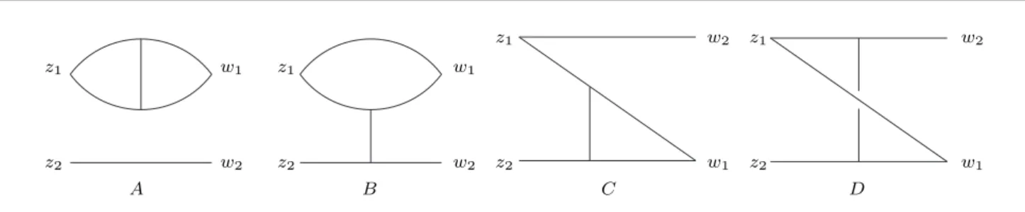
Fig. 5 One loop correction to the correlator of the divergence of conformal operatorsh∂O_j⁽ⁿ⁾(x)∂O^{( ¯}_jⁿ⁾(0)i.

(type B). These diagrams have different color factors:

λsλdfor the A - diagrams, andλ²_sfor the B - diagrams.

All diagrams of the A - type have the diagram we have just now discussed as a subgraph. The only differ- ence is that in order to kill terms linear inδone has to consider an average of the diagrams, (D(δ)+D(−δ))/2.

Forδ=ǫ/2 each of the diagrams,D(±δ), can be sim- plified with the help of the star–triangle relation and rewritten in the form of “sl(2)” diagrams. These diagrams in turn can be calculated up to O(ǫ²) terms in a manner described above. So we skip all details and present the result for each diagram in Appendix C.

All diagrams of B-type shown schematically in Fig. 6 contain two 2 → 1 subgraphs. The diagrams depicted on the right panel are finite while those on the left panel are divergent. The calculation of these diagrams does not present any problem so that we give only final results in Appendix C.

Finally, it follows from Eq. (52) that the sum of counterterm diagrams to the diagrams in Figs. 5 and 6 can be written in the form

2(Z3Z₁⁻¹Zj−1)h∂O⁽ⁿ⁾_j (x)∂O_j^(¯ⁿ⁾(0)i^(ǫ)₀ . (91) Here Zj is the one–loop renormalization constant for the operatorOj,

Zj = 1−u ǫ

λs

(j+ 1)(j+ 2) (92)

and

Z1= 1−uλs

12ǫ +O(u²), Z3= 1−uλd

4ǫ +O(u²). (93) We have put the superscript (ǫ) to the correlator in order to stress that even the tree–level correlator depends onǫthrough a space-time dimensiond= 6−2ǫ.

6 Results

The coefficient T_j⁽²⁾ in the ratio of the correlators is given by the sum of terms in Eqs. (74), (81), (89), (C.13) and (C.14). In the case of operators with other isotopic

symmetry these expressions have to be modified. One can separate seven different isotopic projections

Oâb_f (x;z1, z2) = (Pf)âb_a′b^′ϕâ^′(x+z1n)ϕ^b^′(x+z2n), (94)

wheref = 1, . . . ,7. The projectors Pf can be found in Ref. [16]. The one–loop anomalous dimension for the operatorO^(f)_j is given by

γ_j^f(1)=1 6

λ1− 12λf

(j+ 1)(j+ 2)

, (95)

where λf are the eigenvalues of the operator R^ab

a^′b^′ = d^aa^′^cd^bb^′^con the invariant subspaces,RPf =λfPf. The explicit expressions forλfcan be found in [16]. We note also thatλs=λ1 andλd = 2λ3.