Collinear matching for Sivers function at next-to-leading order

JHEP05(2019)125

Published for SISSA by Springer

Received : January 23, 2019 Revised : May 1, 2019 Accepted : May 11, 2019 Published : May 21, 2019

Collinear matching for Sivers function at next-to-leading order

Ignazio Scimemi,

Andrey Tarasov

and Alexey Vladimirov

a

Departamento de F´ısica Te´ orica, Universidad Complutense de Madrid (UCM) and IPARCOS, E-28040 Madrid, Spain

b

Physics Department, Brookhaven National Laboratory, Upton, NY 11973, U.S.A.

c

Institut f¨ ur Theoretische Physik, Universit¨ at Regensburg, D-93040, Regensburg, Germany

E-mail: ignazios@fis.ucm.es, atarasov@bnl.gov, alexey.vladimirov@ur.de

Abstract: We evaluate the light-cone operator product expansion for unpolarized trans- verse momentum dependent (TMD) operator in the background-field technique up twist-3 inclusively. The next-to-leading order (NLO) matching coefficient for the Sivers function is derived. The method, as well as many details of the calculation are presented.

Keywords: NLO Computations, Deep Inelastic Scattering (Phenomenology)

ArXiv ePrint: 1901.04519

JHEP05(2019)125

Contents

1 Introduction 1

2 Sivers effect and TMD factorization 3

2.1 Sivers function in SIDIS 3

2.2 Sivers function in DY 4

2.3 TMD evolution and operator product power expansion 5 3 Operator definitions for unpolarized and Sivers TMD distributions 7

3.1 Definition of TMD distributions 7

3.2 Evolution and renormalization 9

4 Light-cone OPE at leading order 11

4.1 Light-cone OPE in a regular gauge 11

4.2 Light-cone OPE in the light-cone gauge 13

4.3 Light-cone OPE for the gluon TMD operator 15

5 Light-cone OPE at next-to-leading order 16

5.1 OPE in background field method 17

5.2 QCD in background field 18

5.3 Evaluation of diagrams 19

5.4 Treatment of rapidity divergences 22

5.5 Renomalization 25

5.6 Difference in the evaluation of DY and SIDIS operators 26

6 Definition of collinear distributions 27

6.1 Quark distributions 27

6.2 Gluon distributions 30

7 Small-b expansion for unpolarized and Sivers distributions 32 7.1 From operators to distributions and tree level results 33

7.2 Results at NLO 35

7.3 Discussion and comparison with earlier calculations 36

8 Conclusion 38

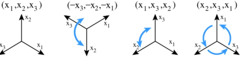
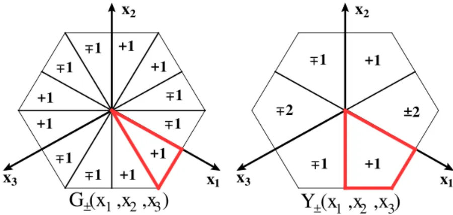
A Parametrization of twist-3 operators and decomposition of 3-tensors 39

B Example of evaluation: diagram E 41

B.1 Evaluation of contribution to OPE 41

B.2 Evaluation of matrix element 44

JHEP05(2019)125

C Diagram-by-diagram expressions 46

C.1 Expressions for OPE 46

C.2 Expressions for TMD distributions 49

1 Introduction

The exploration of the internal structure of nuclei is a fascinating task, which identifies transverse momentum dependent (TMD) distributions as one of its most powerful tools.

Transverse momentum dependent factorization theorems present a consistent description of double-inclusive processes, such as Drell-Yan/Vector/Scalar boson production(DY) [1, 2]

and semi-inclusive deep inelastic scattering (SIDIS) [1, 3, 4] in the regime of small transverse momentum. Within the TMD factorization approach, the information on hadron structure is encoded in TMD parton distribution functions (TMDPDFs) and TMD fragmentation functions (TMDFFs). The presence of the transverse scale allows to resolve the internal structure of hadron with more details than collinear parton distributions. Many polar- ization phenomena, which are subleading in collinear factorization, are described by the leading order TMD factorization. In this work, we study the Sivers function [5, 6], which describes the correlation of an unpolarized parton transverse momentum and a hadron polarization vector.

The Sivers function is an essential part of the single-spin asymmetry (SSA) phe- nomenon. Experimentally, SSA has been measured in SIDIS at Hermes [7], COMPASS [8, 9], JLab [10] and in Drell-Yan at RHIC [11–13]. Its measurement is planned also for the fu- ture Electron-Ion Collider (EIC) [14]. SSA has been also an object of intensive phenomeno- logical analysis, see e.g. [15–20]. The resulting predictions differ substantially among these studies owing to TMD evolution [21], which shows the importance of a correct treatment of QCD perturbatively calculable parts. In the literature, there are several available cal- culations of the SSA in perturbative QCD. The leading order (LO) (and partially the next-to-leading order (NLO)) calculations for the SSA were performed in many works [22–

28]. In principle, following these works it is possible to obtain the perturbative expression for Sivers function at NLO (however, different schemes are used for different parts of the calculation, see discussion in section 7.3). Therefore, the SSA and the Sivers function are probably one of the most renowned and intensively studied polarized TMD quantities.

Although the TMD distributions are genuine non-perturbative functions that should

be extracted from data, they can be evaluated in a model-independent way in terms of

collinear distributions in the limit of large-q

[29], or small-b in the position space. This

procedure is called “matching” and typically it serves as an initial input for the non-

perturbative model of the TMD distributions, see e.g. [17, 30, 31]. The matching greatly

increases the agreement with data [30]. From the theory side, the matching procedure

consists in the selection of the leading term in the light-cone operator product expansion

(OPE) for the TMD operators [32, 33]. Alternatively, the matching can be obtained by

JHEP05(2019)125

taking the small-q

limit of collinear factorization [27, 28], which, however, is not always possible [34].

Only a few TMD distributions of leading-dynamical twist match the twist-2 collinear distributions. These are the unpolarized, helicity and transversity TMDPDFs and TMDFFs. The matching coefficients for these distributions are known uniformly at the next-to-leading order (NLO) [1, 2, 33, 35, 36] and some are known at NNLO [32, 37, 38].

The remaining TMD distributions match twist-3 collinear distributions (apart of the pret- zelosity which is apparently of twist-4 [38, 39]). The knowledge of the matching for these distributions is very poor: the quark TMDPDFs are all known at LO [22, 23, 26, 40, 41]

and only Sivers function is known at NLO [27, 28] (however, see discussion in section 7.2).

The matching for some of quark TMDFFs, such as Collins function, is known at LO [40].

The matching for the majority of gluon TMD distributions is unknown.

The importance of the computation of the perturbative part of a TMD distribution in order to meet an agreement between theory and experiment has been shown already in [30] for the unpolarized case. Depending on the experimental conditions, the measured data can be sensitive to various aspects of the theory such as power corrections in the evolution [42], power correction [43], small-x effects in the evolution [44] and many others.

The full control of all of these sources of non-perturbative physics requires an accurate setting of the perturbative scales, as provided, for instance, by the ζ-prescription of [45].

In this work, we perform a complete NLO computation of the Sivers function starting from its operator definition and performing a light-cone OPE in background field [46]. To our best knowledge, this approach is used for the description of TMD operator for the first time, despite the fact that it is a standard tool in higher twist calculation, see e.g. [47, 48].

This technique grants an unprecedented control of the operator structure and it allows a very general treatment for twist-3 distributions. Therefore, the result obtained in this work is also interesting for a broader study. For the first time, we demonstrate how the TMD renormalization (ultraviolet and rapidity renormalization [49]) is organized at the operator level. We also articulate the role of the gauge links and their direction and show (at the level of operators) the famous sing-change in-between DY and SIDIS definitions of the Sivers function [50]. Motivated by these considerations, we provide a detailed and pedagogical explanation of the calculation method, which is a major target of this article.

For that aim, the Sivers function represents an ideal case, because one can cross-check the calculation with other methods already used in the literature. We anticipate that our results agree with the results present in the literature only partially, however, the origin of the discrepancy is clear.

The article is organized as following. Section 2 is a general introduction to SSA in the

TMD factorization approach. Here we collect the expressions for SSA structure functions

and describe the role of Sivers function and its collinear matching. In section 3.1 we intro-

duce and describe in detail the operator that defines Sivers function. Its renormalization

properties are discussed in section 3.2. Section 3.2 is devoted to the detailed derivation of

OPE at LO. We discuss separately the evaluation in regular (section 4.1) and light-cone

(section 4.2) gauges. The NLO evaluation is presented in section 5. We make a pedagogical

introduction to the background field method in section 5.1–5.2. The details on the NLO

JHEP05(2019)125

evaluation of diagrams are given in section 5.3. In section 5.4–5.5 we discuss the appearance of rapidity divergences and their renormalization. The difference in the evaluation of DY and SIDIS operators is discussed in section 5.6. The extra details on the calculation are given in appendices B, where we present a step-by-step calculation of a diagram and C.1, where we give the diagram-by-diagram expressions for OPE. The collinear distributions are defined in section 6. Additional details of the parametrization definition are given in appendix. A. The transition from operators to distributions is discussed in section 7.1 and the collection of diagram-by-diagram expressions can be found in appendix C.2. The final result of calculation is given in section 7.2. The discussion and comparison with earlier calculations is given in 7.3.

2 Sivers effect and TMD factorization

TMD distributions are defined by a large set of parameters: collinear momentum fraction x, transverse distance b (or transverse momentum p

), polarization, parton flavor f , the type of hadron h, ultraviolet and rapidity renormalization scales (µ and ζ ) and the defining process (DY or DIS). An explicit designation of all these parameters would lead to a heavy notation such as

f

(x, b; µ, ζ ),

which should be read as the Sivers function for a quark q with momentum faction x at the transverse parameter b produced by hadron h in the DY kinematics, measured at scales µ and ζ. Most of this information is not needed in perturbative calculations and in the following we skip the unnecessary parts of the notation, e.g. the renormalization scales are usually dropped. We also distinguish the momentum and coordinate space TMD distributions only by their arguments. In the rest of this section we show how the Sivers function arises in SIDIS and DY cross sections.

2.1 Sivers function in SIDIS

The semi-inclusive deep inelastic scattering (SIDIS) is a common name for a set of processes l(l) + N (P ) → l(l

) + h(P

) + X, (2.1) where l(l

) is a lepton, N is a nucleon target and h is the produced hadron. The TMD factorization is applicable in the regime |P

| Q, where Q

= (l − l

)

is a hard scale of the scattering, P

is the transverse component of the momentum P

. In the following, we use the bold font notation for the transverse components of vectors.

In the case of unpolarized lepton beam, unpolarized produced hadron h and a trans-

versely polarized target N , the cross-section for SIDIS contains three structures. The so-

called Sivers effect (proportional to sin(φ

−φ

)), Collins effect (proportional to sin(φ

+φ

))

and the sin(3φ

− φ

) asymmetry. The structure functions corresponding to these effects

within TMD factorization can be found e.g. in [4, 15, 51]. The structure function for the

JHEP05(2019)125

Sivers effect is denoted by F

. Within the TMD factorization it is [4]

F

(x, z, Q, P

) = −xH

(Q, µ) X

f

e

Z

d

pd

kδ

p − k − P

z

× P

· p

M |P

| f

(x, p; µ, ζ

)D

(z, k; µ, ζ

) +O

P

z

Q

, (2.2)

where the variables x and z are the momentum fractions of partons and M is the hadron mass. The functions D

and f

are unpolarized and Sivers TMD distributions. The factorization scale µ is typically chosen to be of order Q. The scales of soft exchanges (rapidity factorization) ζ

satisfy ζ

ζ

= Q

.

The TMD factorization is naturally formulated in position space, where the Fourier convolution in eq. (2.2) turns into a product of functions. In position space the structure function reads

F

(x, z, Q, P

) = ixM H

(Q, µ) X

f

e

Z d

b

(2π)

e

(2.3)

× P

· b

|P

| f

(x, b; µ, ζ

)D

(z, b; µ, ζ

) + O P

z

Q

. The functions D

and f

depend only on the length of the vector b but not on its direction and one can also simplify the angular dependence [41, 52]

F

(x, z, Q, P

) = −xM H

(Q, µ) X

f

e

Z

0

d|b|

2π |b|

J

|b||P

| z

(2.4)

×f

(x, b; µ, ζ

)D

(z, b; µ, ζ

) + O P

z

Q

, where J

is the Bessel function of the first kind. The equation (2.4) is the usual starting point for the parametrization of the Sivers effect in TMD factorization.

2.2 Sivers function in DY

The Sivers effect also appears in the Drell-Yan/vector boson production process

h

(P

) + h

(P

) → Z/γ

(q) + X → l(l) + ¯ l(l

) + X, (2.5) where one of the initial hadrons is polarized [51, 53–55]. In general one refers to structure functions F

when the hadron h

is polarized and F

when the hadron h

is polarized.

The structure function F

in TMD factorization (i.e. for q

Q) reads [56]

F

(Q, q

) = −H

(Q, µ) N

X

f

e

Z

d

k

d

k

δ

(q

− k

− k

) (2.6)

× q

· k

M |q

| f

(x

, k

; µ, ζ

)f

b

(x

, k

; µ, ζ

) + O q

Q

,

JHEP05(2019)125

where Q

= (l + l

)

is the hard scale of the process, x

are momentum fractions of partons, q

is the transverse component of q = l + l

relative to the scattering plane and f

is the unpolarized TMD distribution. The factorization scales are defined similarly to the SIDIS case, i.e. µ ∼ Q and ζ

ζ

= Q

. The transformation of the structure function under interchange of the polarized hadron (h

↔ h

) is F

= −F

.

The structure functions can be also written in the form F

(Q, q

) = iM H

(Q, µ)

N

X

f

e

Z d

b

(2π)

e

q

· b

|q

| (2.7)

×f

a;DY

(x

, b; µ, ζ

)f

(x

, b; µ, ζ

) + O q

Q

, and

F

(Q, q

) = −M H

(Q, µ) N

X

f

e

Z

0

d|b|

2π |b|

J

(|b||q

|) (2.8)

×f

a;DY

(x

, b; µ, ζ

)f

b

(x

, b; µ, ζ

) + O q

Q

, where we have integrated out the angular dependence.

The Sivers functions in SIDIS, eq. (2.2) and DY, eq. (2.6), have different labels that specify the processes. These functions have different operator definitions (see section 3.1).

However, de facto, the process-dependence reduces to a simple sign change [22, 50, 57, 58]

f

(x, b; µ, ζ) = −f

a;DIS

(x, b; µ, ζ). (2.9) In the following, we demonstrate the origin of the sign-change at the level of OPE.

2.3 TMD evolution and operator product power expansion

The practical application of TMD factorization relies on the concept of TMD evolution, which allows to relate structure functions at different values of Q. Here, we should stress that a TMD distribution is an involved non-perturbative function. In fact, in addition to the non-perturbative structure of TMD distribution (which involves the dependence on the variables (x, b)), the TMD factorization also contains a non-perturbative part of the evolution factor (which depends only on b). An efficient implementation of the TMD approach should be able to disentangle these non-perturbative contributions. The parametrization and extraction of three non-perturbative functions (two TMD distributions and the evolution kernel) of two variables would be a hopeless task if the TMD factorization would not allow us to separate the problem into pieces.

First of all, the TMD evolution is regulated by two scales (µ, ζ ) and it is process independent. It factors out the non-perturbative evolution effects into an evolution factor which is strictly universal for all structure functions and for all TMD factorizable processes.

Nonetheless, the TMD evolution still non-trivially affects the (x, b) dependence of the

distribution which should be modeled as a function of two variables. To simplify this

procedure one can use any available information that restricts the functional form of the

JHEP05(2019)125

TMD. In particular, at small values of b a TMD distribution can be related to collinear distributions in a model-independent way in perturbation theory. Such a relation has the general form provided by OPE

f(x, b) = C

(x, L

) ⊗ f

(x) + b

C

(x, L

) ⊗ f

(x) + . . . , (2.10) where C

are perturbatively calculable Wilson coefficient functions which depend on b only logarithmically via L

(to be defined in eq. (5.2)), f

are collinear distributions of increasing twist and ⊗ is an integral convolution in the variable x. This expansion is valid only in a certain range of b, say |b| < R, where R is some matching scale. For values of b larger than R TMD distribution is completely non-perturbative. In fact, as the value of b gets closer to R, the contribution of higher order terms in the small-b expansion becomes more important. However, our knowledge of the corresponding higher-twist distributions is very limited.

Thus, it is of practical convenience to use only the first term of the small-b expansion in eq. (2.10) and replace the rest by a generic non-perturbative function, i.e.

f (x, b) = C

(x, L

) ⊗ f

(x)f

(x, b). (2.11) The practical success of such an ansatz can be easily understood if we notice that the main contribution to the Fourier integrals in eqs. (2.4), (2.8) comes from the small-b region.

Therefore, we can expect that the function f

has a simple behavior in x and b, which is indeed confirmed by phenomenological applications of this formula. The details of the modeling procedure which is based on eq. (2.11) are different in different approaches, but the core picture described here remains unchanged.

The small-b matching is an essential part of the modern TMD phenomenology. In ref. [30] a comparison of different orders of the matching to experimental results has been performed. It has been shown that the NLO matching is essential for the predictive power of the approach. The NNLO matching provides further improvements and it can be necessary for the description of the most precise experiments.

The achievable precision can also be affected by the choice of scales in the matching.

Let us also mention that in [45] the authors have proved the possibility to disentangle the procedure of small-b matching and TMD evolution using the ζ-prescription which is not entirely possible in other formulations. The ζ -prescription allows using different pertur- bative orders for TMD evolution and small-b matching. This means that the modeling of the TMD through eq. (2.11) is completely separated from the evolution part of the TMD (that is, the scale choice does not mix up non-perturbative pieces of different origin). This fact results to be extremely useful for phenomenology since it allows to use the highest al- lowed/known expression of evolution [59] in combination with polarized observables whose high perturbative orders are unknown. The universal non-perturbative part of evolution can be extracted from the most precise data (such as Z-boson production at LHC) [60].

Let us conclude this section recalling that the hard coefficient functions H

and H

within TMD factorization are given by the quark form factor evaluated in the different

JHEP05(2019)125

analytical regions. At the NLO they differ only by a π

-term, H

(Q, µ) = |C

(Q

, µ

)|

= 1 + 2a

C

−l

− 3l

− 8 + π

6

+ O(a

), (2.12) H

(Q, µ) = |C

(−Q

, µ

)|

= 1 + 2a

C

−l

− 3l

− 8 + 7π

6

+ O(a

), (2.13) where l

= ln(µ

/Q

) and a

= g

/(4π)

. The NNLO and NNNLO expression can be found in [61].

3 Operator definitions for unpolarized and Sivers TMD distributions

In this section, we introduce and review the main properties of TMD distributions.

3.1 Definition of TMD distributions

Through the article we use the standard notation for the light-cone decomposition of a vector

v

= v

n ¯

+ v

n

+ v

, (3.1) where v

= (nv), v

= (¯ nv) and v

is the transverse component (v

n) = (v

n) = 0. The ¯ vectors n and ¯ n are light-like

n

= ¯ n

= 0, (n¯ n) = 1. (3.2)

Their particular definition is related to the factorization frame of the scattering process.

The transverse part (with respect to vectors n and ¯ n) of the metric and Levi-Civita ten- sors are

g

= g

− n

n ¯

+ ¯ n

n

(n¯ n) ,

= n

n ¯

(n¯ n)

, (3.3)

where

is in the Bjorken convention (

= −

= 1). In four dimensions (with n and ¯ n localized in the plane (0, 3)) both tensors have only two non-zero components, g

= g

= −1 and

= −

= 1.

Since the transverse subspace is Euclidian, the scalar product of transverse vectors is negative, v

< 0. In the following, we adopt the bold font notation to designate the Euclidian scalar product of transverse vectors, i.e. b

= −b

> 0, when it is convenient.

Using this notation, the transverse momentum dependent parton distribution functions (TMDPDFs) for unpolarized quark are defined by the matrix element [1, 2, 62]

Φ

(x, b) (3.4)

= Z dz

2π e

hp, S| T ¯ {¯ q (zn + b) [zn + b, ±∞n + b]}γ

T {[±∞n, 0]q(0)}|p, Si,

where [a, b] are Wilson lines defined in eq. (4.2). The notation ±∞n indicates different

cases of TMD distributions, which appear in different processes. The TMD distributions

JHEP05(2019)125

b

z n q q

DY

b

z n q

q

SIDIS

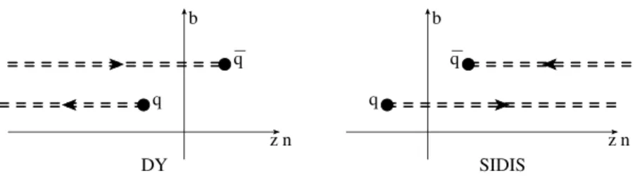
Figure 1. Illustration for the definition of TMD operators in DY and SIDIS. The Wilson lines (shown by dashed lines) are oriented along past (DY) or future (SIDIS) light cone direction. At light-cone infinities the Wilson lines are connected by transverse gauge links (not shown).

that appear in SIDIS have Wilson lines pointing to +∞n, while in Drell-Yan they point to −∞n as in figure 1. The Wilson lines within the TMD operator are along the light-like direction n.

The matrix element in eq. (3.4) for the polarized hadron is parametrized by two inde- pendent functions [41, 52]

Φ

(x, b) = f

(x, b) + i

b

s

M f

(x, b), (3.5) where M is the mass of the hadron and s

is the transverse part of the hadron spin-vector S, i.e. s

= g

S

. The function f

is the unpolarized TMDPDF, which measures the unpolarized quark distribution in an unpolarized hadron. The function f

is known as the Sivers function, which measures the unpolarized quark distribution in a polarized hadron.

The parametrization of eq. (3.5) is given in position space. The distributions in mo- mentum space are defined in the usual manner

Φ

(x, p) =

Z d

b

(2π)

e

Φ

(x, b), (3.6) where the scalar product (bp) is Euclidian. Correspondingly, the momentum space param- eterization reads [4, 63]

Φ

(x, p) = f

(x, p) −

p

s

M f

(x, p). (3.7)

Some explicit relations among particular TMDPDFs can be found in the appendix of ref. [41]. These relations are used to relate structure functions in momentum and coordinate representations in section 2.

The anti-quark TMD distribution is defined as

Φ

(x, b) (3.8)

= Z dz

2π e

hp, S|Tr γ

T ¯ {[±∞n, 0]q

(0)}T {¯ q (zn + b) [zn + b, ±∞n]}

|p, Si.

Using charge-conjugation, one can relate the quark and anti-quark TMD distributions [62], Φ

(x, b) = −

Φ

(−x, b)

, (3.9)

JHEP05(2019)125

from which it follows

f

(x, b) = −f

(−x, b), (3.10) f

(x, b) = f

(−x, b). (3.11) Therefore, in the following we associate the anti-quark distributions with the negative values of x and we define the TMD distributions in the range −1 < x < 1 as

f

(x, b) = θ(x)f

(x, b) − θ(−x)f

(−x, b), (3.12) f

(x, b) = θ(x)f

(x, b) + θ(−x)f

(−x, b). (3.13) The small-b expansion (often called small-b matching or collinear matching) presents a TMD distributions as a series of collinear distributions and Wilson coefficients in the vicinity of b = 0 as in eq. (2.10). For instance, the leading term of the small-b expansion for unpolarized TMD is expressed by the (unpolarized) collinear PDF f

(x)

f

(x, b; µ, ζ) = X

f

Z

dy

y C

(y, b, µ, ζ)f

x y , µ

+ O(b

), (3.14) where the sum index f indicates gluons, quarks and antiquarks of all flavors. The coefficient function C is the perturbative Wilson coefficient, which depends on b logarithmically. Its leading term is δ(1 − y) and the perturbative corrections are known up to NNLO [37]. The power corrections (as in eq. (2.10)) contain collinear distributions of twist-2 and twist-4 and they are currently unknown.

The expression for the small-b matching of the Sivers function is f

= X

f

C

(x

, x

, x

, b, µ, ζ) ⊗ T

(x

, x

, x

, µ) + O(b

), (3.15) where T are the collinear distributions of twist-3, to be defined in sections 6.1, 6.2. The sym- bol ⊗ denotes an integral convolution in the variables x

. At leading order the expression for the coefficient function is known to be ±πδ(x

+ x

+ x

)δ(x

)δ(x − x

) [22, 23, 26, 41]

(and we also re-derive it in the next section). The status of the NLO expressions is cum- bersome. In principle, the quark-to-quark part can be found in [27], where it has been extracted from computation of the cross-section made in [23–25]. However, the computa- tions made in [23–25] miss certain parts and for this reason they are partially incorrect (see extended discussion in [64]). The quark-to-gluon part is evaluated in [28], however, the authors use a scheme which is different from the standard one for twist-2 computations.

We return to this discussion in section 7.2.

3.2 Evolution and renormalization

The renormalized TMD, unlike usual parton distributions, depend on a pair of scales. This

is a consequence of the TMD factorization procedure, which decouples the hard scattering

JHEP05(2019)125

factorization and the factorization of the soft-gluon exchanges [1, 49, 65, 66]. As a result the evolution of TMD is given by a pair of equations

µ

d

dµ

Φ

(x, b; µ, ζ) = γ

(µ, ζ)

2 Φ

(x, b; µ, ζ), (3.16) ζ d

dζ Φ

(x, b; µ, ζ) = −D

(µ, b)Φ

(x, b; µ, ζ), (3.17) where γ

and D are respectively the ultraviolet (UV) and rapidity anomalous dimensions.

Eq. (3.16)–(3.17) are independent of polarization and TMD structure. The double-scale na- ture of factorization and evolution opens also unique possibilities for the phenomenological implementation of TMD. In particular, it allows a universal scale-independent definition of a TMD distribution [45].

At the operator level the double-scale nature of evolution is reflected by the presence of two types of divergences, namely UV and rapidity divergences. Both divergences are to be renormalized. The UV renormalization factor is known as TMD-renormalization factor Z

and it can be extracted from the UV renormalization of quark (or gluon) vertex attached to the (light-like) Wilson line. The rapidity renormalization is made through the rapidity renormalization factor R

(for the proof of multiplicativity of rapidity divergence renormalization, see ref. [49]). It is compulsary that both renormalizations are made at the level of operator and thus do not depend on the hadron states. The renormalized TMD operators U

that defines the physical TMD distribution, reads

U

(x, b; µ, ζ ) = Z

(µ)Z

µ

ζ

R

(b; µ, ζ ) U

(x, b), (3.18) where we explicitly write the scaling variables for each expression. In eq. (3.18) Z

is the renormalization of the field wave functions (Z

for the quark field and Z

for the gluon field). The TMD operators U relevant for this work are defined later in eq. (4.1), (4.3).

Both renormalizations are scheme dependent. We use the conventional MS-scheme together with the dimensional regularization for the UV divergences. For the rapidity renormalization we use the conventional scheme [1, 2, 49, 66, 67] that is fixed by the requirement that no remnants of the soft factor contribute to the hard scattering. Apart from this one should worry about the overlap between collinear and soft modes in the factorization of the cross sections, which is rapidity regulator dependent. This is resolved in the δ-regulator scheme where the form of the rapidity renormalization factor is given by the inverse square root of the TMD soft factor R = 1/ √

S, see ref. [68]. This regulator has been already used several times in higher order calculations, see refs. [32, 37, 38, 68].

The particular expression depends on the order of application of the renormalization factors. In this work, we fix the order as in eq. (3.18) and we use the δ-regularization, whose definition is given in section 5.4. Then the rapidity renormalization factor in MS-scheme reads [49]

R

(b; µ, ζ) = 1+2a

C

B

µ

e

Γ(−)

ln

Bδ

ζ (p

)

− ψ(−) + γ

+O(a

), (3.19)

JHEP05(2019)125

where B = b

/4 and a

= g

/(4π)

. The UV renormalization constant is [32]

Z

Z

µ

ζ

=

1 − C

a

+ O(a

)

1 − 2a

C

1

+ 2 + ln(µ

/ζ )

+ O(a

)

= 1 − a

C

2

+ 3 + 2 ln(µ

/ζ)

+ O(a

). (3.20)

Here, we list only the renormalization constants for quark operators at one-loop, since they are the only required in the present calculation. The gluon case, as well as, two-loop expressions can be found in ref. [32].

We emphasize that the rapidity renormalization factor depends on the boost-invariant combination of scales δ/p

[65] (here, δ regularizes rapidity divergences in n-direction and thus transforms as p

under Lorentz transformations). Such a combination appears in the factorization of the cross section of DY and SIDIS and when splitting the soft factor into parts with rapidity divergences associated with different TMD distributions [2]. In the course of factorization procedure, the accompanying TMD distribution (e.g. D

in (2.4) or f

in (2.8)) gets the rapidity renormalization factor with (δ

/p

) ¯ ζ argument, where δ

regularizes rapidity divergences in ¯ n-direction. The values of p

and p

are arbitrary, however, they dictate the value of ζ and ¯ ζ, since ζ ζ ¯ = (2p

p

)

. The standard and convenient choice of scales is ζ ζ ¯ = Q

, which is the only physical hard scale appearing in the reference processes. This scale determines the value of p

and p

as momenta of partons that couple to test current, see also section 5.4. For an extended discussion see section 6.1.1 in ref. [49] and also refs. [65, 66].

4 Light-cone OPE at leading order

In this section we present the operators that enter in the definition of the Sivers function and their LO limit for small-b, recovering the results of [41]. The notation for operators established in this section is the one used in the NLO computation.

4.1 Light-cone OPE in a regular gauge

Let us denote the operator that defines the TMD distributions in DY case as

U

(z

, z

, b) = ¯ T{ q(z ¯

n + b)[z

n + b, −∞n + b]} γ

T {[−∞n − b, z

n − b]q(z

n − b)}, (4.1) where the Wilson lines are defined as

[a

n + b, a

n + b] = P exp

ig Z

a2

dσn

A

(σn + b)

. (4.2)

The operator that defines the TMD distributions in the SIDIS case reads

U

(z

, z

, b) = ¯ T {¯ q(z

n + b)[z

n + b, +∞n + b]} γ

T{[+∞n − b, z

n − b]q(z

n − b)}.

(4.3)

JHEP05(2019)125

Generally, the links which connect the end points of Wilson lines at a distant transverse plane must be added in both operators (for DY and for SIDIS) [69, 70]. Here, we omit them for simplicity, assuming that some regular gauge (e.g. covariant gauge) is in use. In non- singular gauges the field nullifies at infinities, A

(±∞n) = 0 and the contribution of distant gauge links vanishes. The case of singular gauges is discussed in the following section.

We point out that for convenience of calculation and presentation the operators in eq. (4.1), (4.3) are defined differently in comparison to original operator in eq. (3.4). In particular, we double the transverse distance between fields and write it in symmetric form. Also, the operators in eq. (4.1), (4.3) are defined for arbitrary light cone positions z

and z

, although the definition of a TMD distribution depends only on the difference of these points. Such a generalization does not complicate the calculation, moreover, it allows to cross-check certain results. These modifications are undone on the last step of calculation, see eq. (7.1). Note, that the operators in eq. (4.1), (4.3) define the generalized transverse momentum distributions (GTMDs) and thus the obtained OPE can be applied for generalized TMD (GTMD) kinematics as well.

It is straightforward to check that the spatial separations between any pair of fields in the operators defined in eq. (4.1), (4.3) are space-like.

For that reason we can replace the T - and ¯ T- orderings by a single T -ordering. This significantly simplifies the calculation and in the following we do not explicitly show the symbol of T-ordering, but we suppose that each operator is T-ordered. The possibility to reorder the fields is not a general feature, e.g. TMD operators for fragmentation functions do not allow this simplification and thus, their properties are drastically different.

At LO in perturbation theory one can treat the fields as classical fields, i.e. omit their interaction properties. In this approximation, the small-b expansion is just the Taylor expansion at b = 0. Expanding U in b up to linear terms we obtain

U

(z

, z

, b) = U

(z

, z

, 0) + b

∂

∂b

U

(z

, z

, b)

+ O(b

). (4.4) The leading term is the same for DY and SIDIS cases

U

(z

, z

, 0) = U

(z

, z

, 0) = ¯ q(z

n)[z

n, z

n]γ

q(z

n). (4.5) Note that the half-infinite segments of Wilson lines compensate each other due to the unitarity of the Wilson line and the resulting operator is spatially compact.

The derivative term in eq. (4.4) is different for different kinematics

∂

∂b

U

(z

, z

, b)

= ¯ q(z

n)[z

n, −∞n]( ← − −

∂

− − − →

∂

)γ

[−∞n, z

n]q(z

n), (4.6)

∂

∂b

U

(z

, z

, b)

= ¯ q(z

n)[z

n, +∞n]( ← − −

∂

− − − →

∂

)γ

[+∞n, z

n]q(z

n). (4.7)

1

There is a single exception. The fields of anti-quark operator and the attached Wilson line have light-like

separations but anti-time-ordered. However, the reordering of the operator can performed in the light-cone

gauge, where the gauge links vanish. The detailed discussion on the ordering properties of quasi-partonic

operators can be found in ref. [71].

JHEP05(2019)125

Here, the derivative prevents the compensation of infinite segments of Wilson lines. Acting by derivative explicitly we obtain

∂

∂b

U

(z

, z

, b)

= ¯ q(z

n) ←−

D

[z

n, z

n] − [z

n, z

n] −→

D

γ

q(z

n) (4.8) +ig

Z

−∞

+ Z

−∞

dτ q(z ¯

n)[z

n, τ n]γ

F

(τ n)[τ n, z

n]q(z

n),

∂

∂b

U

(z

, z

, b)

= ¯ q(z

n) ←−

D

[z

n, z

n] − [z

n, z

n] −→

D

γ

q(z

n) (4.9)

−ig Z

z1

+ Z

z2

dτ q(z ¯

n)[z

n, τ n]γ

F

(τ n)[τ n, z

n]q(z

n).

where the covariant derivative and the field-strength tensor are defined as usual

−

→ D

= − →

∂

− igA

, ← − D

= ← −

∂

+ igA

, F

= ∂

A

− ∂

A

− ig[A

, A

]. (4.10) The operators which contribute to each order of the small-b expansion have different geo- metrical twists.

In particular, the first term in eq. (4.8) is a mixture of twist-2 and twist-3 operators, while the second term is a pure twist-3 operator (the same for eq. (4.9)). The procedure of separation of different twist contributions is explained in details in [41]. In the present paper, we skip this discussion because the Sivers function contains only contri- bution of geometrical twist-3 operator. Indeed, comparing the results for DY in eq. (4.8) and SIDIS in eq. (4.9) kinematics we observe that the first terms are the same, while the last terms differ. Therefore, already at this stage it is clear that the Sivers function is made of the operators from the last terms, i.e. pure twist-3 operator.

4.2 Light-cone OPE in the light-cone gauge

Before entering a detailed description of the background field method it is convenient to formulate the derivation of the small-b limit of the TMD functions at LO in the light-cone gauge. This gauge will then be used in the following to describe the background fields.

The definition of TMD operators is gauge invariant. In order to demonstrate this explicitly, let us restore the formal structure of gauge links in eq. (4.1), (4.3). We have

U

(z

, z

, b) = (4.11)

¯

q(z

n+b)[z

n+b, −∞n+b][−∞n+b, −∞n−b][−∞n−b, z

n−b] γ

q(z

n − b),

U

(z

, z

, b) = (4.12)

¯

q(z

n+b)[z

n+b, +∞n+b][+∞n+b, +∞n−b][+∞n−b, z

n−b] γ

q(z

n − b).

Notice, that in order to write eq. (4.11), (4.12) we have explicitly used the fact that the T- ordering can be removed. In the absence of such assumption the finite distance transverse link must be replaced by two half-infinite links [69].

2

By the term geometrical twist we refer to the standard definition of the twist as “dimension minus

spin” of the operator. This definition is formulated for a local operator, but it can be naturally extended

to the light-cone operators as a generating function for local operators.

JHEP05(2019)125

The light-cone gauge is defined by the condition

n

A

(x) = A

(x) = 0. (4.13)

The application of this condition removes the contribution of gauge links along vector n in the TMD operator, i.e. [zn + b, ±∞n + b] = 1 and [±∞n − b, −zn − b] = 1. However, the status of the transverse gauge links is unresolved. This reflects the known fact that the gauge fixing condition (4.13) does not fix the gauge dependence entirely but should be supplemented by an additional boundary condition. There are two convenient choices for boundary conditions in our case

retarded: g

A

(−∞n) = 0, (4.14)

advanced: g

A

(+∞n) = 0. (4.15)

Clearly, each of these boundary conditions is advantageous in some particular kinematics.

As so, we apply the retarded boundary condition for the DY operator. That is, the transverse link at −∞n vanishes,

U

(z

, z

, b) = ¯ q(z

n + b) γ

q(z

n − b), in the retarded light-cone gauge. (4.16) Whereas for the SIDIS operator we apply the advanced boundary condition. That is, the transverse link at +∞n vanishes,

U

(z

, z

, b) = ¯ q(z

n + b) γ

q(z

n − b), in the advanced light-cone gauge. (4.17) Thus, the operators have the same expression in different gauges. In order to recover the structure of gauge links (and hence to obtain the explicitly gauge-invariant operators), we can make a gauge transformation of the operator and subsequently replace each gauge- transformation factor by a Wilson line along the vector n to the selected boundary.

The OPE in the light-cone gauge has a compact form. The leading term of eq. (4.4) is U

(z

, z

, 0) = ¯ q(z

n) γ

q(z

n). (4.18) The expression for the derivative of the operator is also independent of the underlying kinematics (compare to eq. (4.6), (4.7))

∂

∂b

U

(z

, z

, b)

= ¯ q(z

n)( ← − −

∂

− − − →

∂

)γ

q(z

n), (4.19) and in fact, it already gives the final expression of the correction linear in b in the light- cone gauge.

Let us show how the results for LO OPE in eq. (4.8), (4.9) are recovered starting from eq. (4.19). One starts rewriting eq. (4.19) explicitly in a gauge-invariant form. With

3

The names selected here could be misleading since the limit is taken along the light cone, rather then

along a time axis. Also the vector boundary condition assumption is too strong. The quantized Yang-Mills

condition g

A

could be replaced by a weaker ∂

g

A

as it is shown in [72]. Nonetheless, for our purposes

the condition in eq. (4.14), (4.15) is sufficient.

JHEP05(2019)125

this purpose we replace the partial derivatives in eq. (4.19) with covariant derivatives, see eq. (4.10), by adding (and subtracting) appropriate gluon fields

∂

∂b

U

(z

, z

, b)

= ¯ q(z

n)( ←−

D

− −→

D

− igA

(z

n) − igA

(z

n))γ

q(z

n). (4.20) To proceed further, we have to recall the used boundary condition in the form

A

(x) = − Z

−∞

dσ F

(σn + x), in the retarded light-cone gauge, (4.21) A

(x) =

Z

dσ F

(σn + x), in the advanced light-cone gauge, (4.22) where x is an arbitrary point. Substituting these expressions into eq. (4.20) we arrive to eq. (4.8), (4.9).

4.3 Light-cone OPE for the gluon TMD operator

The small-b OPE at NLO contains both quark and gluon collinear operators. The gluon operators that appear in a quark TMD are those that would appear in the small-b OPE for gluon TMD operator. Since this expansion for gluons has never been considered in the literature we briefly describe it here.

We define the gluon TMD operator as (compare to eq. (4.1), (4.3))

G

(z

, z

, b) = F

(z

n+b)[z

n+b, −∞n+b][−∞n−b, z

n−b]F

(z

n−b), (4.23) G

(z

, z

, b) = F

(z

n+b)[z

n+b, +∞n+b][+∞n−b, z

n−b]F

(z

n−b), (4.24) where the Wilson lines are in the adjoint representation, i.e. the contraction of the color indices

is F

(z

)[. . .]

F

(z

). The parametrization of the corresponding TMD matrix elements can be found e.g. in [36].

The evaluation of the light-cone OPE for gluon operators is totally analogous to the one made in section 4.1. The only difference is that the quark fields are replaced by F

and the covariant derivatives act in the adjoint representation. We obtain the following analog of eq. (4.8), (4.9)

∂

∂b

G

(z

, z

, b)

= F

(z

n) ← −

D

[z

n, z

n] − [z

n, z

n] − → D

F

(z

n) (4.25) +ig

Z

−∞

+ Z

−∞

dτ F

(z

n)[z

n, τ n]F

(τ n)[τ n, z

n]F

(z

n),

∂

∂b

G

(z

, z

, b)

= F

(z

n) ← −

D

[z

n, z

n] − [z

n, z

n] − → D

F

(z

n) (4.26)

−ig Z

z1

+ Z

z2

dτ F

(z

n)[z

n, τ n]F

(τ n)[τ n, z

n]F

(z

n), where the covariant derivatives are in the adjoint representation. Alike the quark case, the only operators which contribute to the Sivers function are given in the second lines of these equations.

4

This is the only color structure that appears in the leading power of TMD factorization. The so-called

dipole TMD distributions that couples to opposite directed Wilson lines in the fundamental representation

do not appear in the factorization of SIDIS or DY processes.

JHEP05(2019)125

5 Light-cone OPE at next-to-leading order

The object of this section is to introduce the calculation of OPE for U up to terms linear in b at NLO in perturbation theory. The OPE is realized when b

Λ

and it looks like

U (z, b) = X

n

C

(z, L

, a

(µ)) ⊗ O

(z; µ) (5.1) +b

X

n

C

(z, L

, a

(µ)) ⊗ O

(z; µ) + O(b

),

where C are the coefficient functions which depend on b

logarithmically, n enumerates all available operators at this order and ⊗ is some integral convolution in variables z. Here, we also introduce the notation for the coupling constant a

= g

/(4π)

and for the logarithm combination that typically enters in perturbative calculations

L

= ln

µ

b

4e

. (5.2)

The variable µ represents the scale of OPE.

The complexity of the computations for OPE increases drastically passing from LO to NLO in perturbative QCD. In the latter case one cannot omit the field interactions, as it happens in ordinary Taylor expansion as in eq. (4.4). The propagation of fields between different points is responsible of the fact that eq. (4.4) is to be modified in the presence of interactions which can pick up additional fields from the vacuum. Moreover, the OPE with interacting fields contains all possible operators with correct (as prescribed by the theory) quantum numbers.

An additional difficulty in the present calculation is that only a few computing methods

have been tested on higher twist operators. For the twist-2 TMD operators the matching

procedure is simple because in the OPE a TMD is in a one-to-one correspondence with the

on-shell matrix elements over collinear-parton states. In the case of higher twist operators

the only matrix elements of collinear partons are not suitable for obtaining the matching

coefficients, since a transverse component of momentum is needed to carry the operator

indices. It can also happen that a matrix element over collinear partons is not infrared-safe

and it requires an additional regularization with a (specific) separation of pole contribu-

tions, see e.g. [24, 73]. These problems are solved using off-shell matrix elements, which

is significantly more complicated, due to the fact that the higher-twist operators mix with

each other via QCD equations of motion and that off-shell colored states are not generally

gauge invariant. The best method to evaluate the coefficient functions at higher twist re-

sults to be the background-field method. At the diagram level, the method is equivalent to

the evaluation of a generic matrix elements, with the main difference that the result of the

calculation is given explicitly in operator form. The method allows to keep track of gauge

properties and significantly simplifies the processing of equations of motion. Altogether,

these properties make the background-field method very effective for higher twist calcula-

tions. In the following we concentrate on this method, for which we provide a brief general

introduction in section 5.1. The details of the calculation are given in section 5.2–5.3. The

JHEP05(2019)125

treatment of rapidity divergences and renormalization needs a special discussion which is provided in section 5.4–5.5. All the computation is done for the DY case, but the passage to the SIDIS case does not present particular difficulties and the comparison of the two cases is provided in section 5.6.

5.1 OPE in background field method

The background-field method is founded on the idea of mode separation. The operator matrix element between states S

and S

is defined as

hS

|U |S

i = Z

DΦ Ψ

1

[Φ] U [Φ] Ψ

[Φ] e

, (5.3) where the letter Φ represents any QCD field {¯ q, q, A

}, Ψ

is the wave function of the state S and S is the action of QCD. Let us split the fields into the “fast” and “slow” (or

“short-correlated” and “long-correlated” in position space terminology) components, as

Φ(x) = ϕ(x; µ) + φ(x; µ). (5.4)

Here, the “fast” modes φ have momentum p > µ, while “slow” modes have momentum p < µ. The (factorization) scale µ is not explicitly defined but it is large enough to guarantee the convergence of the perturbative series. In the following we omit the argument µ for the fields. We postulate that physical states (hadrons) are built from the “slow”

components, i.e. Ψ

[Φ] = Ψ

(ϕ) so that eq. (5.3) turns into hS

|U |S

i =

Z

Dϕ Dφ Ψ

[ϕ] U [ϕ + φ](x) Ψ

[ϕ] e

. (5.5) In this expression the integral over “fast” components can be evaluated and the expression for observables has the following effective form

hS

|U |S

i = Z

Dϕ Ψ

[ϕ] U e [ϕ](x) Ψ

[ϕ] e

, (5.6) where

U e [ϕ](x) = Z

Dφ U [ϕ + φ](x) e

. (5.7)

The mode separation then assumes that the “slow” fields can be treated as free-fields on distances x

. This hypothesis is typical for effective field theories (see for instance [74–76]

for the application of similar concepts in soft collinear effective theory (SCET) or [48] for TMD factorization at small-x).

One can interpret the construction in eq. (5.6) as an evaluation of the perturbative

QCD fields in a general parton background, which gives the method its name. After the

integration of the “fast” fields in eq. (5.6), the resulting effective operator is then expanded

using free-theory twist expansion, as it was done in section 4. It is important to realize

that in background calculation the result is gauge-invariant and satisfies QCD equations

of motion at each step of the evaluation (even for each diagram). The result then is also

JHEP05(2019)125

universal, that is, it is valid for all states (we do not even specify them) and thus, we can operate only with fields ϕ. Essentially, the background field methods is concentrated in a single definition, eq. (5.6).

The background field method is an essential tool of the modern small-x calculations.

In this case the separation of kinematic modes is based on the strong ordering in rapidity, which is a distinctive feature of the small-x kinematics. To define different modes one has to introduces a rapidity cutoff parameter σ, which separates “fast” (p

< σ) and “slow” (p

>

σ) fields based on the value of the longitudinal component of the momenta p

. Instead of the twist expansion the calculation of the functional integral over “fast” fields (5.6) is now performed in the so-called shock-wave approximation. Since the procedure of separation of modes is quite general, the method can incorporate different kinematic regimes, which has been recently employed in [44, 48].

5.2 QCD in background field The QCD Lagrangian reads

L = ¯ q(i 6D)q + 1

4 F

F

+ gauge fix, (5.8) where the covariant derivative and F

are defined in eq. (4.10). Following the mode separation we split the fields as A

→ A

+ B

and q → q + ψ, where ψ and B

are

“fast” fields and q and A

are “slow” (background) fields. The separation of modes in the main body of the Lagrangian is straightforward, but the gauge fixing term should be considered with caution. The ultimately convenient point of the background field method is the possibility to choose different classes of gauge fixing for different modes. The detailed discussion on gauge fixing in QCD with background method is given in [77, 78].

We choose the most convenient combination of gauges for our task. For “fast” com- ponents we use the background-field gauge,

(∂

δ

+ gf

A

)B

= D

[A]B

= 0 , (5.9) which is the analog of covariant gauge fixing in the usual QCD perturbation theory. In particular, the propagator has the familiar form

B

(x)B

(0) =

Z d

k

(2π)

e

−iδ

k

+ i0

g

− (1 − α) k

k

k

+ i0

, (5.10)

where α is a free parameter. For background fields we use light-cone gauge eq. (4.13) with retarded boundary condition eq. (4.21) for DY operators and advanced boundary condition eq. (4.15) for SIDIS operators.

In background field formulation, the Lagrangian of QCD splits into three parts L = L[q, A] + L[ψ, B] + δL, (5.11) where the first two terms are usual QCD Lagrangians built for particular modes and the last term is the “fast-slow” modes interaction,

δL = g q ¯ 6 Bψ + ¯ ψ 6 Bq + ¯ ψ 6 Aψ

+ δL

+ δL

+ δL

, (5.12)