One-loop Chern-Simons terms in ﬁve dimensions

(1)

MPP-2013-3 CERN-PH-TH/2013-022

One-loop Chern-Simons terms in five dimensions

Federico Bonetti¹, Thomas W. Grimm² and Stefan Hohenegger³

1 2 Max-Planck-Institut f¨ur Physik, F¨ohringer Ring 6, 80805 Munich, Germany

3 Department of Physics, CERN - Theory Division, CH-1211 Geneva 23, Switzerland

ABSTRACT

We compute one-loop corrections to five-dimensional gauge and gravitational Chern- Simons terms induced by integrating out charged massive fields. The considered massive fields are spin-1/2 and spin-3/2 fermions, as well as complex two-forms with first order kinetic terms. Consistency with six-dimensional gravitational anomalies of (1,0) and (2,0) theories is shown by interpreting the massive fields as excited Kaluza-Klein modes in a circle compactification. The results are in accordance with the geometric predictions of the M-theory to F-theory duality as well as the comparison with an explicit one-loop computation in heterotic string theory compactified on K3×S¹.

February, 2013

1bonetti@mpp.mpg.de

2grimm@mpp.mpg.de

3stefan.hohenegger@cern.ch

arXiv:1302.2918v1 [hep-th] 12 Feb 2013

(2)

Contents

1 Introduction 2

2 Summary of results 4

3 Field theory computation 6

3.1 Minimally coupled massive actions . . . . 6

3.2 Computation of theA∧F ∧F coupling . . . . 7

3.3 Computation of theA∧tr (R∧R) coupling . . . . 11

3.4 Non-minimal couplings and renormalisation . . . . 15

4 Consistency with the M-theory to F-theory limit 16 4.1 Field theory prediction . . . . 16

4.2 F-theory check . . . . 18

5 Dual heterotic string on K3×S¹ 21 5.1 Heterotic setup . . . . 22

5.2 String amplitudes . . . . 22

5.2.1 Vertex operators . . . . 22

5.2.2 World-sheet CFT . . . . 23

5.2.3 Explicit amplitudes . . . . 24

5.3 Change of basis . . . . 25

6 Conclusions 26 A Notations and conventions 27 B Gravitational perturbative expansion 29 C Feynman rules 29 C.1 Spin-1/2 fermion . . . . 30

C.2 Massive self-dual tensor . . . . 31

C.3 Spin-3/2 fermion . . . . 32

D Torus integration 33

(3)

1 Introduction

The derivation of a Wilsonian low-energy effective action amounts to integrating out all excitations beyond a chosen cutoff mass scale and obtaining a theory with modified couplings for the remaining degrees of freedom. The consideration of such theories is crucial, for example, to study physical properties of a fundamental theory such as string theory at low energies. The corrections to the low energy effective action obtained by integrating out massive fields are organised in an expansion in the inverse mass scale.

In the limit of large cutoff scale corrections are typically strongly suppressed and can be neglected. In this case all modes with masses above the cutoff scale become effectively non-dynamical and can be decoupled from the theory. This is the subject of well known results in quantum field theory, such as the Appelquist-Carazzone-Symanzik decoupling theorem [1]. This reasoning, however, breaks down for certain types of couplings. Four- dimensional examples are furnished by Goldstone-Wilczek currents [2] and Wess-Zumino terms [3] generated by integrating out a fermion that becomes massive via Yukawa coupling to a scalar that gets a non-vanishing VEV. They are independent of the fermion mass and have to be included in the low-energy effective action even in the limit in which it is taken to infinity. In this work we will study couplings with similar features, namely gauge and gravitational Chern-Simons couplings in five-dimensional theories.

The five-dimensional quantum field theories under consideration will propagate both massless and massive degrees of freedom. We will consider massive spin-1/2 fermions, spin-3/2 fermions, and complex two-forms. The kinetic and mass terms of the fermions are of standard form while the complex two-forms admit first order kinetic terms. The latter feature is possible in odd-dimensional theories and is crucial for the fields to introduce corrections to Chern-Simons couplings. This can be attributed to the fact that the Chern-Simons couplings violate parity and only fields with parity violating actions can modify their prefactors when deriving the Wilsonian effective action. The massive fields are minimally coupled to a masslessU(1) gauge fieldAwith field strength F. We aim to derive the corrections to the gauge Chern-Simons term A∧F ∧F and the gravitational Chern-Simons term A∧tr (R∧R), where R is the five-dimensional curvature two-form, induced by integrating out all massive fields. After appropriate overall normalisation each of the massive fields yields an integer contribution to the Chern-Simons couplings.

This is consistent with the topological nature of the Chern-Simons couplings that implies that their prefactors are quantised and turn out to be independent of the mass scale of the fields that are integrated out. As a consequence, they survive the limit in which the mass scale is taken to infinity. The results for the gauge Chern-Simons coupling were given in [4] without proof. This work substantiates our claims and extends them to include gravitational couplings. Our findings are summarised in section 2.

This analysis is not purely academic, since, remarkably, these couplings elegantly encode information about higher-dimensional anomalies after Kaluza-Klein compactification. In particular, we can consider a six-dimensional theory compactified on a circle to get a five-dimensional quantum field theory which propagates both massless and mas-

(4)

sive degrees of freedom. Six-dimensional gravitational anomalies are thus associated to the five-dimensional Chern-Simons couplings induced by integrating out excited Kaluza- Klein modes. Gauge anomalies can be accessed in the five-dimensional setup as well. In this case the massive degrees of freedom can also arise from spontaneous gauge symmetry breaking.

As already explained in [4] (see also [5]), a heuristic explanation for the above mentioned connection between five-dimensional Chern-Simons terms and six-dimensional anomalies can be obtained by considering the one-loop diagram necessary to determine the latter. Indeed, in six dimensions, the gravitational anomaly is captured by a four- point amplitude with external graviton legs. The polarisations of the latter have to be contracted in all possible ways and thus particularly also include contributions corresponding to the compact S¹ direction. From the five-dimensional perspective, the four- point function therefore decomposes into a sum of correlators involving (five-dimensional) gravitons, the Kaluza-Klein vector A, and the graviscalar, which we will consider to be non-dynamical and replace by the radius r. Focusing on terms which break five- dimensional parity, we are naturally lead to consider Chern-Simons terms of the form A∧F ∧F and A∧tr (R∧R), where R is the five-dimensional curvature two-form and F the field-strength tensor corresponding to A. One-loop corrections to these couplings are therefore expected to encode information about higher-dimensional anomalies. We will have more to say about this interesting connection in the upcoming paper [6].

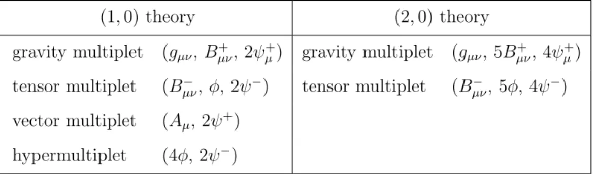
There are various ways to embed our five-dimensional or six-dimensional setup into string theory and M-theory. We will consider two realisations in this work. Firstly, we will realise the five-dimensional setup by compactification of M-theory on an elliptically fibered Calabi-Yau threefold. Using the M-theory to F-theory limit reviewed in [7] the resulting low-energy effective action for the massless fields should be identified with the low energy effective action of a six-dimensional F-theory compactification on a circle after all Kaluza-Klein modes are integrated out. The Chern-Simons couplings on the M-theory side are determined by the intersection numbers and the second Chern class of the Calabi-Yau threefold [8, 9, 10]. We thus find a purely geometric computation of the total Chern-Simons contribution for (1,0) theories on a circle and agreement with our field theory computation can be shown.

A second string theory realisation of our setup can be found by considering heterotic string theory on K3×S¹ in the absence of NS5-branes (see e.g. [11] for earlier computations in this setting). In this case the underlying six-dimensional (1,0) theory is a theory with one self-dual and one anti-self dual tensor. The contributions to the five-dimensional Chern-Simons terms can in this case be computed as a three-point amplitude at one-loop.

It turns out that the computation is largely insensitive to most of the details of the internal world-sheet CFT which allows us to calculate the amplitudes explicitly for generic points of the moduli space of K3 compactifications. The summation over the various massive modes propagating through the loop in the field theory picture corresponds to integrating over the moduli space of world-sheet tori from the string perspective that captures the contribution of all CFT excitations. We manage to perform this integration

(5)

explicitly and find again agreement with our field theory result.

The paper is organised as follows. Section 2 summarises the main results of the paper. The families of massive fields that can generate one-loop Chern-Simons terms are listed in table 2.1, while table 2.2 gives the Chern-Simons coefficient for each of them.

Section 3 contains the Feynman diagram computation of these coefficients. Section 4 discusses the check of the field theory results in the framework of six-dimensional F- theory compactifications. Section 5 is devoted to the explicit one-loop computation of the relevant amplitudes in heterotic string theory onK3×S¹. Finally, in the conclusions we recapitulate our results and discuss briefly further directions. The main body of the paper is accompanied by several appendices. Notations, conventions, and other useful identities are collected in appendices A and B. The complete Feynman rules used in section 3 are gathered in appendix C. In appendix D we perform the calculation of a torus integral that appears in the string theory computation.

2 Summary of results

Let us start by summarising the results of this paper. The object of our investigation are five-dimensional theories in which some massive fields are coupled to a U(1) gauge field Aµ and to the metric gµν. In particular, we study how quantum corrections due to massive fields can generate the Chern-Simons couplings

SAF F =kAF F

Z

A∧F ∧F , SARR =kARR

Z

A∧tr (R∧R) (2.1) in the low energy effective action. In these expressions F = dA is the field strength of the U(1) gauge field and R denotes the curvature two-form built from the metric gµν.

We show that three classes of massive fields are capable of generating such Chern- Simons terms in the quantum effective action: massive spin-1/2 fermions ψ, massive self-dual tensors Bµν, and massive spin-3/2 fermions ψµ. By massive self-dual tensor we mean a complex two-formBµν that admits a non-standard first order kinetic term ¯B∧dB together with a mass termmB¯∧∗B. Its free equation of motion thus reads schematically

∗dB ∝mB . (2.2)

These tensor fields and their coupling to a U(1) gauge field has been analysed in [12, 4].

Further details about massive self-dual tensors are given in section 3.1. We refer to these fields as self-dual because they can be thought of as the excited Kaluza-Klein modes of a six-dimensional self-dual tensor compactified on a circle.

Spin-1/2 fermions, self-dual tensors, and spin-3/2 fermions can be characterised in terms of associated representations of the massive little group in five dimensions,SO(4)∼= SU(2)×SU(2). Such representations are labelled by a pair of half-integer spins (j1, j2).

The correspondence between massive fields and SO(4) representations is summarised in table 2.1.

(6)

field free EOM SO(4) rep.

spin-1/2 fermion ψ (∂/−c1/2m)ψ = 0 ¹₂,0

or 0,¹₂ self-dual tensor Bµν (∗d−icBm)B = 0 (1,0) or (0,1) spin-3/2 fermion ψµ (γ^ρµν∂µ+c3/2mγ^ρν)ψν = 0 ¹₂,1

or 1,¹₂ Table 2.1: Summary of massive representations considered in this work.

We have included the equation of motion that puts each field on-shell in the absence of interactions. The coefficients c1/2, cB, c3/2 can take the values ±1 and determine which SO(4) representation is realised. Note that here and in the following m denotes the mass of the physical one-particle states and is thus taken to be positive. The pairs of representations (j1, j2) and (j2, j1) are interchanged under parity. Correspondingly, these classes of fields break parity at tree level. From this point of view, the fact that couplings of the form (2.1) are generated in the effective action can be interpreted as a parity anomaly: quantum effects compensate for the parity violation originally induced by these families of massive fields, after they are integrated out.

The following table summarises our findings for the coefficients kAF F, kARR of the induced Chern-Simons couplings in (2.1). Coefficientsc1/2,cB,c3/2 correspond to those in table 2.1. The symbolqdenotes theU(1) charge of the massive fields. It is a dimensionless

spin-1/2 fermion ψ self-dual tensor Bµν spin-3/2 fermion ψµ

kAF F = − 1

48π² q³·c1/2 − 1

48π² q³ ·(−4cB) − 1

48π² q³·(5c3/2) kARR= − 1

384π²q·c1/2 − 1

384π² q·(8cB) − 1

384π² q·(−19c3/2) Table 2.2: Summary of the one-loop contributions for various fields.

quantity and its normalisation is fixed by the minimal coupling prescription ∂µ →∂µ− iqAµ. The derivation of these results is the subject of the upcoming sections. Nonetheless, let us stress here two crucial aspects of the computation. Firstly, kAF F and kARR are quantum corrected at one-loop only. This is expected by arguments involving locality of the effective action and quantisation of the Chern-Simons couplings [13] and is consistent with the interpretation in terms of parity anomalies in five dimensions.

Secondly, our results are derived using a simple quadratic action for the massive fields, which only includes minimal coupling to the gauge fieldAµ and the metricgµν. We argue that kAF F and kARR are indeed insensitive to any fine detail of the interactions. For the kAF F coupling, the effect of some non-minimal interactions is analysed explicitly in section 3.4. It is shown there that such non-minimal couplings do not affect the renormalised

(7)

value of kAF F. These features are expected for topological couplings such as (2.1) that can be interpreted as parity anomalies.

Note that we refrain from a discussion about the possibility to write down fully consistent interacting theories for the three classes of massive fields under examination.

For instance, it is expected that an interacting theory of massive spin-3/2 fermions is only possible in presence of (possibly spontaneously broken) supersymmetry, even though our findings are independent of the precise way it is realised in the five-dimensional action.

From this point of view, we do not consider other parity-violating representations of SO(4), such as (³₂,0) or (2,0), because no example is known of consistent interacting theories for the corresponding massive fields.

3 Field theory computation

In this section we compute the coefficients of the Chern-Simons couplings (2.1) in perturbative quantum field theory. We start by reviewing the actions for the massive spin-1/2 fermion, self-dual tensor, and spin-3/2 fermions minimally coupled to the U(1) gauge field and the metric. We then describe the main points of the Feynman diagram calcula- tions for the gauge and the gravitational Chern-Simons terms. We conclude the section by studying the effect of some non-minimal couplings on the gauge Chern-Simons term.

3.1 Minimally coupled massive actions

The Chern-Simons couplings (2.1) can be captured by one-loop computations in a theory where the massive fields considered above are minimally coupled to theU(1) gauge field Aµ and the metric gµν. In this section we briefly review the corresponding actions.

A spin-1/2 fermion is described by a five-dimensional Dirac spinor ψ. In order to couple it to the metricgµν we have to introduce a vielbeine^aµ. The action forψminimally coupled to the U(1) gauge field Aµ and the vielbein e^aµ is taken to be

S1/2 = Z

d⁵x e

−ψγ¯ ^µD^µψ +c1/2mψψ¯

, c1/2 =±1, (3.1) where e = dete^aµ, γ^µ = γ^aeaµ, and where we have introduced the full spacetime and U(1) covariant derivative

D^µψ =∂µψ+¹₄ωµabγ^abψ−iqAµψ . (3.2) On the right hand side, ωµab is the Levi-Civita spin connection constructed from the vielbein, and q is the U(1) charge of the fermion ψ. More details about our spacetime and gamma-matrix conventions can be found in appendix A. As stated in section 2, mis the positive physical mass and c1/2 labels two inequivalent spinor representations of the massive little group SO(4) in five dimensions. Under a parity transformation, the sign of c is reversed.

(8)

Let us now turn to massive self-dual tensors in five-dimensions. Their action, including the coupling to a U(1) gauge field, can be written as [4]

SB = Z

d⁵x√

−g

−¹₄icB^µνρστB¯µνD^ρBστ −¹₂ mB¯µνB^µν

, cB =±1 . (3.3) The relevant part of the spacetime and U(1) covariant derivative reads

D[ρBµν]=∂[ρBµν]−iqA[ρBµν] . (3.4) Note thatg = detgµν and that^µνρστ denotes the five-dimensional Levi-Civita tensor. In our conventions, it satisfies ⁰¹²³⁴=−1/√

−g if 0, . . . ,4 are curved indices. Note that in this case parity violation is not due to the mass term, but to the kinetic term.

Finally, a spin-3/2 fermion is described by a Dirac vector-spinor ψµ with action S3/2 =

Z

d⁵x e

−ψ¯ργ^ρµνD^µψν −c3/2mψ¯µγ^µνψν

, c3/2 =±1, (3.5) where the antisymmetric part of the spacetime and U(1) covariant derivative is given by D^[µψν] =∂[µψν]+ ¹₄ω[µ|abγ^abψν]−iqA[µψν] . (3.6) In analogy with the spin-1/2 case, the two inequivalent representations of SO(4) differ by the sign of the mass term.

3.2 Computation of the A∧F ∧F coupling

The U(1) Chern-Simons couplingA∧F ∧F does not involve the gravitational field. As a consequence, throughout this section we can ignore the coupling of massive fields to gravity and take gµν =ηµν. No distinction between flat and curved indices is made. The coupling to Aµ can be treated perturbatively in the framework of quantum field theory on flat spacetime.

The coefficient of the A∧F∧F term in the quantum effective action can be extracted from the three-point function of the gauge fieldAµ. More precisely, we work in momentum space and we denote by ΓAAA the sum of 1PI Feynman diagrams with three external vectors with incoming momenta p1,p2,p3 and polarisation vectors e1, e2, e3. The Chern- Simons term

kAF F

Z

A∧F ∧F =−kAF F

Z

d⁵x ^µνρστAµ∂νAρ∂σAσ (3.7) in the effective action corresponds to a contribution to ΓAAA of the form

ΓAAA⊃i3!×(−kAF F)λτ µ1µ2µ3p^λ₁p^τ₂e^µ₁¹e^µ₂²e^µ₃³ , (3.8) where we have included a factor ofifrom the Feynman rules and the combinatorial factor 3! to take into account symmetry under permutations of the three vectors. Contributions

(9)

A(p3, e3) A(p2, e2)

A(p1, e1)

k

Figure 1: One-loop Feynman diagram involved in the computation of the Chern-Simons coefficient kAF F. The external lines are three vectors A with incoming momenta p1, p2, p3 and polarisation vectorse1, e2,e3. The internal lines can represent a massive spin-1/2 fermion, a massive self-dual tensor, or a massive spin-3/2 fermion. The loop momentum k flows in the direction of the arrow.

to ΓAAA different from (3.8) will be ignored. They correspond to higher-derivative and non-local terms in the effective action. As already mentioned, we expect that the right hand side of (3.8) is corrected at one loop only. As shown in sections 4 and 5 our one-loop results pass non-trivial tests in the framework of F-theory and heterotic string theory.

We can derive Feynman rules using the actions (3.1), (3.5) and (3.3) evaluated in flat spacetime and extract the propagators for massive fields, together with the interaction tri-vertex among two massive fields and one gauge field Aµ. These propagators and vertices are listed in appendix C.

At the one-loop level, only one class of diagrams can be built using the interaction vertices at hand. A representative diagram is depicted in figure 1. Wiggly lines represent the external vectors, while solid lines represent massive fields. Each class of massive fields contributes separately to the amplitude. To get the full answer, it has to be summed with the analog diagram where the orientation of the loop is reversed. This is equivalent to swapping the labels 1 and 2 on the external legs. Since the relevant structure in (3.8) is invariant under this relabelling, the loop-reversed diagram simply gives an overall additional factor 2.

The denominator of the diagram (which is determined through its propagator factors) is the same for all fields running in the loop. If the labelling of figure 1 is adopted, it is given by

D= 1 k²+m²

1 (k−p2)²+m²

1

(k+p1) +m² , (3.9) which is to be completed by a suitable numerator factor N which particularly encodes information about the vertices and is strongly dependent on the fields running in the loop.

In (3.9), the usual Feynman i prescription is understood. We make use of Schwinger

(10)

parameterisation to unify denominators, and write D= 1

m⁶ Z ∞

0

dα Z ∞

0

dβ Z ∞

0

dγ e^{−(α+β+γ)(`}²^+∆)/m² . (3.10) In this expression, α, β, γ are dimensionless parameters, and we have made use of the shorthand notations

`=k−yp2+zp1 , ∆ = m²+ 2yzp1 ·p2+y(1−y)p²₁+z(1−z)p²₂ , (3.11) where y=β/(α+β+γ) andz =γ/(α+β+γ). The full diagram is then given by

I=D·N= 1 m⁶

Z ∞

0

dα Z ∞

0

dβ Z ∞

0

dγ

Z d⁵`

(2π)⁵ e^{−(α+β+γ)(`}²^+∆)/m²N , (3.12) where, of course, the numerator is different for different species of massive fields running in the loop. We also note that the sum of the diagram in figure 1 with the diagram with the opposite orientation has a distinct symmetry with respect to exchanging the external points. On general grounds, one can show that this symmetries restrict the parity violating part of the integrand in (3.12) at the bilinear level in the external momenta to only depend on the Schwinger parameters in the combination (α+β+γ). This is a useful consistency check we have applied throughout the computations.

By naive power-counting arguments, we do not expect any infrared divergence in this one-loop diagram, but we cannot exclude the possibility of ultraviolet divergences.

If Schwinger parameterisation is used, the integral over the loop momentum ` contains an exponential factor and (after Wick rotation) is convergent as long as α+β +γ is strictly positive. Ultraviolet divergences are translated into divergences in the α, β, γ integration, coming from the region where these three parameters are simultaneously small. We regularise the amplitude by cutting out this portion of the α, β, γ integration domain with a step-function: in (3.12) we make the replacement

Z ∞

0

dα Z ∞

0

dβ Z ∞

0

dγ →

Z ∞

0

dα Z ∞

0

dβ Z ∞

0

dγ θ(α+β+γ −), (3.13) where >0 is the regulator.

Recall from (3.8) that we are only interested in the coefficient of a term with two powers of external momenta contracted with an-symbol. This allows us to simplify the computation of the diagram.

First of all, only the terms that contain an-symbol have to be kept in the numerator.

If a self-dual tensor runs in the loop, the -symbol is introduced directly at the level of Feynman rules both in the propagator and in the vertex. When a spinor runs in the loop, the -symbol is generated by traces of gamma matrices. This follows from the identities tr 1 = 4, trγ^µ¹^µ²^µ³^µ⁴^µ⁵ = 4i ^µ¹^µ²^µ³^µ⁴^µ⁵ , trγ^µ¹^...µ^p = 0 for p= 1,2,3,4. (3.14) We see that only those terms need to be retained that contain an odd number of gamma matrices greater than or equal to five.

(11)

Second of all, we can perform a formal power series expansion of (3.12) in p1,p2 and we can neglect all terms that are not bilinear in p1 and p2. In particular, this implies that we can use the approximation ∆≈m², since all other terms in the exact expression (3.11) for ∆ would generate additional powers of external momenta of the form p²₁, p²₂, orp1·p2.

Finally, by symmetry arguments (not spoiled by our choice of regulator), we can make the following replacements in the numerator under theR

d⁵` integral:

`µ1. . . `µr →0 ifr is odd ,

`µ`ν → ¹₅`²ηµν , `µ1`µ2`µ3`µ4 → ₃₅¹ (`²)²(ηµ1µ2ηµ3µ4 +ηµ1µ3ηµ2µ4), . . . (3.15) All tensor integrals in the loop momentum are thus reduced to scalar integrals.

The calculation of the diagram is now straightforward but tedious.⁴ After the numerator algebra is performed and the replacements (3.15) are made, the integrals over the loop momentum and the Schwinger parameters are computed using the formulae

Z d⁵`

(2π)⁵ e^{−(α+β+γ)`}²^/m²(`²)ⁿ= im²ⁿ⁺⁵ 24π³

Γ(n+ 5/2)

(α+β+γ)^n+5/2 , (3.16)

Z ∞

0

dα Z ∞

0

dβ Z ∞

0

dγ θ(α+β+γ−) e^{−(α+β+γ)}

(α+β+γ)^aαⁿ¹βⁿ²γⁿ³ =

= Γ(1 +n1)Γ(1 +n2)Γ(1 +n3)

Γ(3 +n1+n2+n3) Γ(3 +n1+n2+n3−a;) . (3.17) We have performed the usual Wick rotation `⁰ → i`⁰ in the first integral and have introduced the incomplete gamma function

Γ(x;) = Z ∞

dτ τ^x−1e^−x (3.18)

in the second integral.

Let us consider the diagram where the spin-1/2 fermionψ runs in the loop. By power- counting we expect a quadratic divergence, since the numerator has up to three powers of the loop momentum. The parity-violating part of the numerator, however, turns out to be of zero-th order in the loop momentum, thus giving a finite result without the need of any regulator.

This does not hold for the diagrams where Bµν and ψµ run in the loop. In fact, even though the parity-violating part of the numerator has a better UV behaviour than the full diagram, it still contains terms proportional to `² or (`²)². This implies that both diagrams have a divergent piece. In our regularisation scheme such divergences appear as coefficients of negative powers of the regulator in a formal expansion of the diagram.

4We made use of theMathematicapackagesxTensorof the bundlexAct[14] andGAMMA[15].

(12)

We can then give the -expansion for all the three species under consideration: spin- 1/2 fermions ψ, tensors Bµν, and spin-3/2 fermions ψµ,

(diagram)1/2 = i

64π² c1/2q³

+ 4 +O(^1/2)

, (3.19) (diagram)B = i

64π² cB q³

+ 15

√π^−1/2 −16 +O(^1/2)

, (3.20) (diagram)3/2 = i

64π² c1/2q³

− 105 4√

π^−3/2 + 15 4√

π^−1/2 + 20 +O(^1/2)

. (3.21) Note that the factor (−1) for a fermionic loop has been taken into account, but we have not inserted the overall factor 2 due to the diagram with the reversed loop orientation.

In order to extract the physical observable kAF F from these expressions we adopt a minimal subtraction prescription: negative powers of in the expansion are discarded.

This gives the results of table 2.2. In section 3.4 we discuss the effect of non-minimal couplings and show how they can be used to cancel divergences.

3.3 Computation of the A∧tr (R∧R) coupling

Let us now turn to the discussion of the mixed U(1)-gravitational Chern-Simons term A∧tr (R∧R). To compute its coefficient we treat the coupling of massive fields to gravity perturbatively. The metric is written as

gµν =ηµν+hµν , (3.22)

and computations are performed order by order in a formal power series inhµν around flat spacetime. Indices µ, ν, . . . are thus raised and lowered with ηµν and its inverse and no distinction is made between flat and curved indices. Further details about the expansion inhµν are collected in appendix B.

WhenA∧tr (R∧R) is expanded according to (3.22) terms with arbitrarily high powers ofhµν are generated, because of the non-linear dependence of the Riemann tensor on the metric. Nonetheless, in order to read off the Chern-Simons coupling we can restrict to the lowest order term,

kARR

Z

A∧tr (R∧R) = (3.23)

=−¹₂kARR

Z

d⁵x ^µ¹^µ²^µ³^µ⁴^µ⁵Aµ1∂λ∂µ2hτ µ3

∂^τ∂µ4h^λµ5 −∂^λ∂µ4h^τµ5

+O(h³) . As a consequence, the constant kARR can be extracted from the sum of 1PI Feynman diagrams with one vector and two gravitons, denoted ΓAhh. More precisely, the sought-for Chern-Simons coupling corresponds to the contribution

ΓAhh⊃i2!× ¹₂kARRµ0µ1µ2λτp^λ₁p^τ₂(p1ν2p2ν1 −ην1ν2p1·p2)e^µ₀⁰e^µ₁¹^ν¹e^µ₂²^ν² , (3.24)

(13)

where p1, p2 are the incoming momenta of the gravitons, e0 is the polarisation tensor of the vector, and e1, e2 are the symmetric polarisation tensors of the gravitons. The prefactor i2! comes from the standard Feynman rule prescriptions. Any term that does not match the structure of the right hand side of (3.24) will be neglected, since it would correspond to higher-derivative and non-local terms in the effective action.

It is interesting to note that the tensor structure in (3.24) is transverse with respect to both the vector and the graviton polarisation tensors, i.e. it vanishes if any of the replacements

e^µ₀ →p^µ₀ =−p^µ₁ −p^µ₂ , e^µν₁ →a^(µp1ν) , e^µν₂ →a^(µp2ν) (3.25) is made, for arbitrarya^µ. It can be shown that this tensor structure is the only structure with an-symbol and four powers of external momenta that has this transversality prop- erty and is symmetric in the exchange of labels 1 and 2. Its appearance is a consequence of gauge invariance. Transversality with respect to e0 reflects invariance of (3.23) under U(1) transformations. Transversality with respect to e1, e2 derives from invariance of (3.23) under diffeomorphisms. Recall that under an infinitesimal diffeomorphism with parameter ξ^µ we have

δhµν = 2∂(µξν)+O(h) . (3.26)

Gauge invariance can be used as a self-consistency check of the Feynman diagram computation. Indeed, we find that the desired contributions to ΓAhh organise into the structure (3.24) after all relevant diagrams are summed.

The Feynman rules needed in the diagrammatic computation of ΓAhh are deduced by expanding the actions (3.1), (3.5), (3.3) for the massive fields according to (3.22). This gives interaction vertices of arbitrarily high powers inhµν but we only need an expansion up to second order in hµν. More precisely, four kinds of vertices are relevant for the calculation of ΓAhh. If we denote any of the massive fieldsψ, Bµν,ψµ as Φ, we need: the gauge tri-vertex ¯ΦΦA, already considered in the previous section; the gravitational tri- vertex ¯ΦΦh; the purely gravitational quadri-vertex ¯ΦΦhh; the mixed gauge-gravitational quadri-vertex ¯ΦΦAh. All such vertices are collected in appendix C.

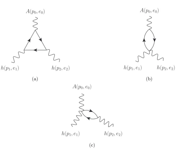
The presence of quadri-vertices enlarges the family of one-loop Feynman diagrams that can be built. In particular, we have three different topologies, depicted in figure 2.

The total amplitude is given by the sum

2(a) + (b) + 2(c) , (3.27)

where diagram (a) is counted twice because of the two possible orientations of the loop, and diagram (c) is counted twice according to which graviton is connected to the mixed quadri-vertex.

For each diagram, denominators can be unified by means of Schwinger parameters. In diagram (a) three parameters are needed, as in the previous section, while diagrams (b) and (c) require only two parameters. Up to minor changes, the methods described in the

(14)

h(p₂, e₂) h(p₁, e₁)

A(p₀, e₀)

(a)

h(p₂, e₂) h(p₁, e₁)

A(p₀, e₀)

(b)

h(p₂, e₂) h(p₁, e₁)

A(p₀, e₀)

(c)

Figure 2: One-loop Feynman diagrams involved in the computation of the Chern-Simons coefficientkARR. The external line on top represents a vectorAwith incoming momentum p0 and polarisation vector e0. The other external lines are gravitons h with incoming momentap1,p2and symmetric polarisation tensorse1,e2. The internal lines can represent a massive spin-1/2 fermion, a massive self-dual tensor, or a massive spin-3/2 fermion.

(15)

previous section can be applied straightforwardly to the diagrams at hand. In particular, UV divergences in diagrams (b) and (c) are regulated by means of the replacement

Z ∞

0

dα Z ∞

0

dβ →

Z ∞

0

dα Z ∞

0

dβ θ(α+β−), (3.28) where α, β are the Schwinger parameters and is the regulator. For the sake of com- pleteness, we record the two-parameter analog of the identity (3.17),

Z ∞

0

dα Z ∞

0

dβ θ(α+β−) e^−(α+β)

(α+β)^aαⁿ¹βⁿ² =

= Γ(1 +n1)Γ(1 +n2)

Γ(2 +n1+n2) Γ(2−a+n1+n2;). (3.29) Let us stress an important difference between the present computation and the one discussed in the previous section. In the case of the gauge Chern-Simons couplings, the relevant tensor structure (3.8) does not contain any product of external momenta. This allowed us to use the approximation ∆≈m² in the computation of the diagram in (3.12).

In the present case, one of the two parts of the gauge invariant tensor structure (3.24) is proportional to p1·p2. This implies that we have to keep the p1 ·p2 term inside ∆ and expand e^(α+β+γ)`²^/m² (or e^(α+β)`²^/m²) in a power series in the external momenta. This is indeed crucial to obtain the gauge invariant structure (3.24) after all the three diagrams are combined according to (3.27).

As in the case of the gauge Chern-Simons term, the parity violating part of the diagrams has a better UV behaviour than expected from naive power-counting. Nev- ertheless, the diagrams in which the self-dual tensor and the spin-3/2 fermion run in the loop have some divergent parts. After all diagrams are summed according to (3.27) and the total expression is organised in powers of , the⁰ coefficient is proportional to the gauge-invariant combination (3.24), while negative-power coefficients are not gauge- invariant. This leads us to apply a minimal subtraction prescription and simply drop the unphysical divergent pieces. In this way the results of table 2.2 are obtained.

Let us conclude this section with a side remark. Recall from section 3.2 that the relative weight between the diagram for spin-1/2 and spin-3/2 fermion contributions to kAF F is five. This result can be derived straightforwardly from an alternative form of the massive action for a spin-3/2 ψµ,

S_3/2⁰ = Z

d⁵x e

−ψ¯ργ^µD^µψ^ρ+c3/2mψ¯ρψ^ρ

, c3/2 =±1. (3.30) Indeed, when this action is evaluated on a flat background, it gives exactly the same propagator and vertex as the spin-1/2 action (3.1), up to a factor of the metricηµν.

Remarkably, the alternative action (3.30) gives also the correct relative weight −19 between the spin-1/2 and the spin-3/2 contributions to kARR. This claim has been