Effective action of 6D F-theory with U(1) factors: Rational sections make Chern-Simons terms jump

arXiv:1305.1929v1 [hep-th] 8 May 2013

MPP-2013-125

Effective action of 6D F-theory with U(1) factors:

Rational sections make Chern-Simons terms jump

Thomas W. Grimm, Andreas Kapfer and Jan Keitel

Max-Planck-Institut f¨ ur Physik,

F¨ohringer Ring 6, 80805 Munich, Germany

ABSTRACT

We derive the six-dimensional (1, 0) effective action arising from F-theory on an ellip- tically fibered Calabi-Yau threefold with multiple sections. The considered theories admit both non-Abelian and Abelian gauge symmetries. Our derivation employs the M-theory to F-theory duality in five-dimensions after circle reduction. Five-dimensional gauge and gravitational Chern-Simons terms are shown to arise at one-loop by integrating out mas- sive Coulomb branch and Kaluza-Klein modes. In the presence of a non-holomorphic zero section, we find an improved systematic for performing the F-theory limit by using the concept of the extended relative Mori cone. In this situation Kaluza-Klein modes can become lighter than Coulomb branch modes and a jump in the Chern-Simons levels occurs. By determining Chern-Simons terms for various threefold examples we are able to compute the complete six-dimensional charged matter spectrum and show consistency with six-dimensional anomalies.

May, 2013

1

grimm, kapfer, jkeitel@mpp.mpg.de

Contents

1 Introduction 2

2 On the geometry of Calabi-Yau threefolds with Abelian gauge factors 4

2.1 General remarks on elliptic fibrations . . . . 5

2.2 Topology of elliptically fibered Calabi-Yau threefolds . . . . 6

3 Effective action via M-theory 9 3.1 Reducing (1, 0) supergravity on a circle . . . . 9

3.2 M-theory on a Calabi-Yau threefold with U (1)s . . . . 16

3.3 Classical matching of F-theory and M-theory . . . . 20

4 One-loop Chern-Simons terms and anomaly cancelation 21 4.1 Review of 6D anomalies with U (1)s . . . . 22

4.2 One-loop Chern-Simons terms in circle reduced theories . . . . 24

4.3 Gravitational and mixed anomalies via one-loop Chern-Simons terms . . 26

4.4 Pure gauge anomalies and one-loop Chern-Simons terms . . . . 34

4.5 Creating new Chern-Simons terms for m

> m

. . . . 36

5 Systematics and concrete examples of Calabi-Yau threefolds with Abelian gauge factors 37 5.1 Generalities and an algorithm for determining sign w . . . . 38

5.2 First example: Gauge group SU(2) × U(1) . . . . 40

5.3 Second example: Gauge group SU (5) × U (1)

. . . . 45

5.4 Third example: Gauge group SU(5) × U(1)

. . . . 46

6 Conclusions 48 A Conventions and group theory identities 50 A.1 Conventions . . . . 50

A.2 Group theory identities . . . . 51

B Circle reduction of the 6D action 55

C Loop calculations 60

D Some geometry 62 D.1 Exact identities for the second Chern class . . . . 62 D.2 Toric fans . . . . 63

1 Introduction

Compactifications of F-theory on elliptically fibered Calabi-Yau threefolds have long been known to yield a large class of six-dimensional (6D) supergravity theories with eight supercharges implying N = (1, 0) supersymmetry [1, 2, 3]. These (1, 0) theories are chiral, can admit non-Abelian gauge groups with a charged matter spectrum, and support a number of tensors with self-dual or anti-self-dual field strength. Since F-theory arises from the consistent Type IIB string theory, its effective theories are quantum consistent and meet all known low-energy constraints [4, 5, 6, 7, 8, 9, 10]. In particular, since all fermions in the 6D spectrum are chiral, anomaly cancelation imposes strong constraints on the number of multiplets and their connection to the couplings of the low-energy effective supergravity action. The effective action of F-theory reduced on an elliptically fibered Calabi-Yau threefold with purely non-Abelian gauge symmetries was derived via the duality of F-theory to M-theory in [11, 12, 13]. In this work we generalize the derivation of [12] to include Abelian gauge symmetries and investigate their physics from the F-theory and M-theory point of view.

Recently, global F-theory compactifications with Abelian gauge symmetries arising on seven-brane world-volumes have been investigated intensively [14, 8, 15, 16, 10, 17, 18, 19, 20]

. At weak string coupling, U(1) symmetries arise on stacks of D7-branes and can be analyzed from the global configuration of D7-branes and O7-planes [22, 23, 24]. Their origin in F-theory is purely geometrical, since geometrically massless U (1) symmetries are counted by the number of sections of the elliptic fibration. More mathematically stated, the geometry of the Abelian gauge groups is captured by the rank of the Mordell- Weil group of the elliptic fiber [3, 15, 16]. As we discuss in detail in this work, the properties of the sections parametrizing the U (1)s have a crucial impact on the physics of the low-energy effective action. In particular, we consider non-holomorphic sections defined by rational instead of holomorphic equations. These induce rich new physics in six- and four-dimensional F-theory reductions [16, 10, 17, 18, 19, 20]. Notably, there is no physical reason for the zero section of the Calabi-Yau manifold to be holomorphic and abandoning this constraint leads to interesting new phenomena, which we investigate in this work. The geometry of elliptic fibrations with a non-holomorphic zero section has recently been investigated in [18, 20].

To determine the effective action of F-theory on Calabi-Yau threefolds, one has to consider these reductions as a limit of M-theory [25]. This can be traced back to the fact that there is no fundamental low-energy effective action of F-theory. We thus proceed

2

For a systematic survey of U (1)s in local models see [21].

as follows. Determining the effective action of M-theory on a resolved elliptically fibered Calabi-Yau threefold at large volume allows us to use eleven-dimensional supergravity plus known higher curvature corrections to derive a five-dimensional (5D) effective ac- tion [26, 27]. This action is compared with the low-energy effective action obtained by compactifying a general six-dimensional (1, 0) action with Abelian and non-Abelian gauge groups on a circle. The M-theory reduction and the circle compactification have to be compared in the regime where all massive modes are integrated out. On the circle side this implies that both massive modes arising from moving to the five-dimensional Coulomb branch and the modes arising in the Kaluza-Klein tower have to be integrated out [12]. The classical comparison of the two five-dimensional theories allows deriving the various F-theory couplings specifying the six-dimensional action. Importantly, the loop corrections arising from integrating out the massive modes teaches us about the six-dimensional charged spectrum even in the phase where the Calabi-Yau threefold is smooth.

Before comparing the five-dimensional theories, one first has to integrate out massive modes arising in the Coulomb branch after circle reduction. In order to do that, we compute the one-loop Chern-Simons levels using the general results of [28] (see also ref- erences therein). The massive modes include fields that become massive when moving to the five-dimensional Coulomb branch of the gauge group. These modes can be charged under the non-Abelian as well as the Abelian gauge groups of the six-dimensional theory.

Accordingly, they introduce gauge and gravitational Chern-Simons terms involving the dimensionally reduced Cartan generators of the six-dimensional gauge group. In addi- tion, also all massive Kaluza-Klein modes have to be integrated out. These are charged under the Kaluza-Klein vector arising in the reduction of the six-dimensional to the five- dimensional metric, and may also admit charges under the six-dimensional gauge group.

Integrating out all massive spin–1/2, spin–3/2 and tensor modes, we derive the form of the Chern-Simons levels in the presence of six-dimensional U(1)-symmetries. Since these Chern-Simons terms are independent of the mass scale, one-loop corrections have to be included irrespective of the size of the compactifying circle and the values of the VEVs parametrizing the Coulomb branch vacuum. Supersymmetry further relates classical and one-loop Chern-Simons terms to the kinetic terms. This allows to determine the charac- teristic data specifying the complete six-dimensional (1,0) vector and tensor sector. The hypermultiplet sector can only be studied for the neutral multiplets that reduce triv- ially from six to five dimensions. While the number of charged hypermultiplets can be determined via the one-loop Chern-Simons terms, their precise metric remains elusive.

Having derived the 6D (1,0) spectrum and the characteristic data of the F-theory effective action, one can verify that anomaly conditions are fulfilled. The 6D anomaly conditions were translated into intersection relations in [5, 6, 29, 15], where, however, it was implicitly assumed that the zero section was holomorphic. We show that loop- induced Chern-Simons terms can be employed to analyze equivalent conditions even in the case of a non-holomorphic zero section.

Hence, one particular focus of this work lies on Calabi-Yau threefold examples with

rational sections. In particular, if the zero section is not holomorphic, then certain topological identities used in [15, 12, 9] have to be refined. We show that this has a crucial impact on the F-theory limit and the structure of the five-dimensional one-loop Chern- Simons terms. For a non-holomorphic zero section, one can no longer independently shrink the generic torus fiber of the elliptic fibration and the exceptional divisors resolving the non-Abelian singularity. The physical interpretation of this situation for the circle reduced 6D (1,0) theory is that some of the Kaluza-Klein modes are in fact lighter than the Coulomb branch modes. Let us denote by m

the Coulomb branch mass of a given mode and by m

= 1/r the Kaluza-Klein scale of a circle with circumference r. Then the inequality

m

< m

(1.1)

considered in [12, 10] is no longer satisfied for all states when dealing with a non- holomorphic zero section. The effect of this modified hierarchy is to induce a discrete shift in the one-loop Chern-Simons levels, as was already noted in [10]. In particular, this implies that various cancelations among contributions of Kaluza-Klein modes, which were previously encountered for holomorphic zero sections, do not occur. On the resolved Calabi-Yau threefold, the mass hierarchy is dictated by the Mori cone of the manifold.

We find it necessary to replace the relative Mori cone by a more refined version, the extended relative Mori cone introduced in a different context in [30], which captures not only information about the mass hierarchy among the curves associated to the gauge groups, but also contains data about the zero section.

The paper is organized as follows. To begin with, we review in section 2 the geometric properties of elliptically fibered Calabi-Yau threefolds with rational sections. In section 3 we derive the effective action of 6D F-theory compactifications with Abelian gauge factors by comparing a circle reduced N = (1, 0) supergravity on the Coulomb branch and M- theory on a resolved Calabi-Yau threefold. We proceed in section 4 by including one- loop induced Chern-Simons terms in the circle reduced theory and relating them to 6D anomalies. We formulate the matching of the one-loop Chern-Simons coefficients with the analogous expressions in M-theory. Finally, we verify the matching in some examples in section 5. In all examples we find a connection between the existence of a holomorphic zero section in the geometry and a hierarchy of Coulomb branch masses m

and Kaluza- Klein masses m

. This suggests an improved systematic of performing the F-theory limit.

2 On the geometry of Calabi-Yau threefolds with Abelian gauge factors

In this section we review some of the essential features of elliptically fibered Calabi-Yau

manifolds. In particular, we recall the connection between the Mordell-Weil group of

the elliptic fiber and aspects of Abelian gauge group factors in the resulting effective

theory. Furthermore, we comment on the implications of having a non-holomorphic zero

section, which has recently appeared in examples constructed in [18, 20]. A more detailed geometric discussion of its features can be found in [20]. While much of the following discussion is independent of the dimension of the base manifold, we deal with Calabi-Yau threefolds in this work and hence take dim

B = 2.

2.1 General remarks on elliptic fibrations

A fibered Calabi-Yau threefold is defined by specifying its total space Y

together with a holomorphic and surjective map

π : Y

→ B (2.1)

called the projection map defining the base manifold B. Y

is said to be elliptically fibered if the preimages of points p on B under π are elliptic curves

E = π

(p) for p ∈ B . (2.2)

Up to birational equivalence

, every elliptic curve can be described in terms of a Weier- strass equation

y

= x

+ f xz

+ gz

, (2.3)

where z, x and y are the homogeneous coordinates of P

and f and g are elements of the field K that E is defined over. In terms of the Weierstrass coefficients f and g, the discriminant of the torus is given as

∆ = 4f

+ 27g

(2.4)

and the elliptic curve is singular when ∆ = 0.

Given an elliptic curve E , its Mordell-Weil group MW(E ) is formed by the set

of rational points on E . MW(E ) is a finitely generated Abelian group, and therefore takes the following form

MW(E ) = Z

⊕ T , (2.5)

where r is the rank of the Mordell-Weil group and T is the torsion subgroup, which is the finite Abelian group completing the decomposition.

In our specific case we consider fibrations of E over the base manifold B. K is then the fraction field of the coordinate ring of the base manifold and in order for Y

to be a Calabi-Yau threefold, f and g must be sections of K

and K

, respectively, where K

Two varieties are said to be birationally equivalent if they are isomorphic to each other inside open subsets. Here, openness is to be understood in terms of the Zariski topology, in which every open subset is automatically dense. Therefore two birationally equivalent varieties can only differ inside lower-dimensional subsets.

4

Since two rational points on an elliptic curve can be added to obtain a third rational point, addition

endows this set with a group structure. The neutral element is the zero point on E. For a concrete

example see the appendix of [16].

is the canonical bundle of the base manifold. Rational points, including the zero point on E , then become rational sections of the Calabi-Yau threefold, which we denote by σ

. As explained for example in [16, 17, 18, 20], rational sections do not necessarily define injective maps from the base manifold into the Calabi-Yau threefold anymore. Instead, they are allowed to wrap entire fiber components over certain loci in the base manifold.

Therefore they are only properly defined over the blow-up ˆ B along these loci

σ

: ˆ B → B ֒ → Y

, (2.6) where the first arrow is given by the blow-down map. For Weierstrass models defined by (2.3), the zero section given by [x : y : z] = [1 : 1 : 0] is always holomorphic, as was noted in [20]. However, since an arbitrary elliptic curve can be mapped to such a model only birationally , there exist elliptic fibrations for which none of the sections is holomorphic.

While rational zero sections still describe physically well-defined compactifications

, in most examples in the existing literature the zero section is taken to be holomorphic. We therefore try to make sure to point out the implications of having a non-holomorphic zero section. In particular, we argue that in this case the mass hierarchy (1.1) can be violated.

2.2 Topology of elliptically fibered Calabi-Yau threefolds

Having recalled the key features of an elliptic fibration, we now choose our notation essentially as in [30, 12, 10, 20] and select a convenient basis of divisors. To be able to perform meaningful calculations, we take ˆ Y

→ Y

to be the smooth blow-up of Y

along all singular loci. We then choose the following basis of divisors D

and their respective dual two-forms ω

∈ H

( ˆ Y

, Z ):

• The divisor D

dual to the two-form along which C

is expanded to give the Kaluza- Klein vector field A

. D

is obtained by shifting the zero section D

according to (2.10).

• Vertical divisors D

= π

(D

), α = 1, . . . , h

(B) obtained as pullbacks of a basis of divisors D

on B.

• Exceptional divisors D

obtained by resolving singularities of the elliptic fibration along the divisor S

in the base manifold.

• U (1) divisors D

obtained by applying the Shioda map given in (2.13) to each of the rational sections σ

, where m = 1, . . . , rank MW(Y

).

In order to define the shifts mentioned above, it is convenient to introduce the inter- section product on the base manifold as

D

· D

= (D

· D

)

= D

· D

· D

≡ η

, (2.7)

5

See for example the manifolds in [18, 20].

so that we can lower and raise Greek indices using η

and its inverse, η

. Furthermore, we can project a two-cycle X ⊂ Y

to the base via

π(X) = (X · D

) D

. (2.8) As was noted in [31, 15, 10], D

is obtained by requiring that

D

· D

· D

= 0 , (2.9)

which can be achieved by choosing D

= D

− 1

2 (D

· D

· D

)D

. (2.10) In a similar fashion, the Shioda map shifts the rational sections σ

such that specific intersection numbers of D

with D

, D

and D

vanish, as we will see in (2.17c). This orthogonalization procedure turns out to be crucial for the matching of M-theory and F- theory later. First, however, we must recall the intersection properties of the exceptional divisors obtained by blowing up the singularity of the elliptic fibration. Given a base divisor S

over which the elliptic fiber of Y

develops singularities, the blow-up divisors of ˆ Y

intersect as

D

· D

· D

= −C

S

· D

, (2.11)

where C

denotes the coroot intersection matrix, which we define in the group theory conventions of appendix A.2.

Having associated the exceptional blow-up divisors D

with the Cartan generators of g, one can go a step further and define a rational curve localized over a single point in the base manifold for each root of g. For the simple roots α

of g, one chooses a base divisor D

intersecting S

exactly once and takes the intersection product between D = π

(D

) and D

:

C

= −D

· D for D

· S

= 1 (2.12) From (2.11), one can see that the intersection D

· C

reproduces the Ith component of the simple root α

in the Dynkin basis of the root system of g. With these definitions, we are ready to give an explicit formula for the Shioda map relating rational sections σ

and their associated U(1)-divisors:

D

= σ

− D

− ((σ

− D

) · D

· D

) D

− (σ

· C

) C

D

(2.13)

Let us now discuss the intersection numbers in this basis and emphasize clearly what impact a rational zero section has. We begin by examining the geometry of the blow- up divisors D

. A holomorphic zero section marks a single point in each fiber. In particular, when this point lies over S

, it is on the original fiber component

and not on

6

Assuming that the resolution locus in the base is S

, one can associate the divisor π

(S

) − P

I

D

with the affine node of the Dynkin diagram of g. Intersecting this divisor with π

(D

) such that

D

· S

= 1 gives the rational curve associated with the original fiber component.

the resolution P

s of the rational curves C

. Therefore the following equation holds as an identity in the Chow ring of ˆ Y

:

D

· D

= 0 , if D

is holomorphic. (2.14) On the other hand, a rational zero section may wrap the entire fiber component over lower-dimensional loci of the base. Since this fiber component intersects the resolution divisors as the affine node in the extended Dynkin diagram of g, its intersection can be non-zero. However, since the locus over which a rational zero section can wrap the entire fiber component has at least codimension one in the base and is generically different from S

, D

· D

has at least codimension two in the base manifold. The intersection with a vertical divisor therefore vanishes and we find that

D

· D

· D

= 0 (2.15)

even for a non-holomorphic zero section.

The other peculiarity of having a non-holomorphic zero section is that one can no longer evaluate expressions involving D

by using adjunction to the base manifold. Recall that

D

· D

= D

|

= K

, if D

is holomorphic. (2.16) However, for a rational zero section this needs no longer be the case, since the divisor D

and B are only rationally equivalent, but not isomorphic .

To put it in a nutshell, a rational zero section may intersect blow-up divisors over points in the base and the divisor corresponding to that section is no longer isomorphic to the base manifold. With this in mind, we can now list the intersection numbers both for a rational zero section and for its holomorphic counterpart. We begin by stating intersections that hold both for a rational and for a holomorphic zero section:

D

· D

· D

= 0 , D

· D

· D

= η

, D

· D

· D

= 0 , (2.17a) D

· D

· D

= 0 , D

· D

· D

= 0 , D

· D

· D

= −C

(S

· D

) , (2.17b) D

· D

· D

= 0 , D

· D

· D

= 0 , D

· D

· D

= 0 , (2.17c) D

· D

· D

= π(D

· D

)

. (2.17d) All three equations in (2.17a) describe intersections on the base manifold. The first one is a triple intersection product between codimension 1 objects in the base and therefore vanishes. Using this fact, the second equation simply reduces to the definition in (2.7) and the third equation can be verified directly by inserting (2.10). Next of all, the three equations in (2.17b) are a direct consequence of the blow-up geometry and were discussed above. Equation (2.17d) is just a formal rewriting of the intersection number using (2.8)

7

The Chow ring of an algebraic variety X is formed by equivalence classes of the subvarieties of X ,

where the equivalence relation is given by rational equivalence. The multiplicative structure is defined

by taking the intersection of two subvarieties.

and we stress that unlike in [10], we do not require D

and D

be orthogonal to each other. Lastly, the remaining three equations (2.17c) follow from the orthogonalization properties of the Shioda map. They can be verified by inserting the expression in (2.13) and exploiting that all sections intersect the generic fiber component precisely once, that is

σ

· E = D

· E = D

· E = 1 , (2.18) where the class of the generic fiber E is given as

D

· D

= E η

. (2.19)

In a second step, we now assume to have a holomorphic zero section D

. Using the definition of the Shioda map we evaluate

D

· D

= 0 , if D

is holomorphic. (2.20) Exploiting (2.14), (2.20) and (2.16) one can then show that

D

· D

· D

= − 1

2 π(D

· D

)

K

, D

· D

· D

= 1

2 K

(D

· D

· D

) , (2.21a) D

· D

· D

= 0 , D

· D

· D

= 0 , D

· D

· D

= 0 , (2.21b) D

· D

· D

= 1

4 K

K

, (2.21c)

where K

are the expansion coefficients of the canonical class of B in K

= K

D

. All equations in (2.21b) are a direct consequence of (2.14) and (2.20). Equation (2.21c) follows from applying the adjunction formula. Finally, the two equations in (2.21a) both follow from applying (2.14), (2.20) and the adjunction formula. We stress that (2.21) are not valid for a non-holomorphic zero section.

3 Effective action via M-theory

In this section we perform the circle reduction of a 6D (1, 0) supergravity with Abelian gauge factors describing the F-theory effective action. We push the reduced theory to the Coulomb branch and compare it with M-theory on a resolved elliptically fibered Calabi- Yau threefold. We focus in particular on the Chern-Simons terms and the prepotential of the resulting 5D N = 2 supergravity. On the M-theory side, we find classical terms surviving the F-theory limit and one-loop induced terms that vanish in the limit. In contrast, the F-theory side only accounts for the classical terms in the reduction. By matching the classical terms, we find a geometric interpretation of the 6D F-theory data.

3.1 Reducing (1, 0) supergravity on a circle

The effective action of F-theory compactified on a singular Calabi-Yau threefold is a 6D

(1, 0) supergravity theory. Let us denote the 6D space-time manifold by M

. The (1, 0)

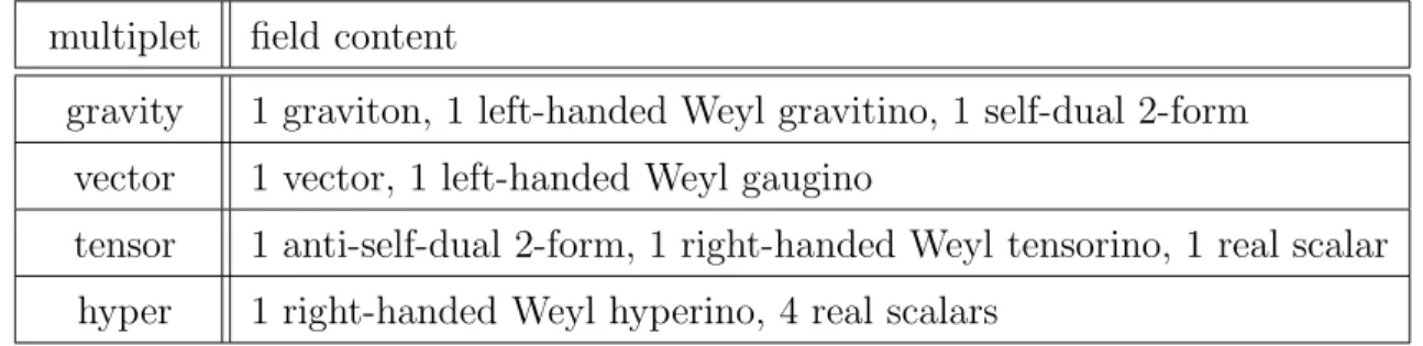
supermultiplets with their individual bosonic and fermionic constituents are listed in the Table 3.1. In the following, we denote the number of vector multiplets by V , the number of tensor multiplets by T , and the number of hypermultiplets by H.

multiplet field content

gravity 1 graviton, 1 left-handed Weyl gravitino, 1 self-dual 2-form vector 1 vector, 1 left-handed Weyl gaugino

tensor 1 anti-self-dual 2-form, 1 right-handed Weyl tensorino, 1 real scalar hyper 1 right-handed Weyl hyperino, 4 real scalars

Table 3.1: The spectrum of 6D (1, 0) supergravity. Note that one can substitute each Weyl spinor by two symplectic Majorana-Weyl spinors.

We allow for a non-Abelian gauge group G, which splits into a simple non-Abelian part G

and n

U (1)-factors as

G = G

× U(1)

. (3.1)

Our goal is to find the F-theory effective action of a (1, 0) theory with gauge group G.

Since the tensors in the spectrum obey (anti-)self-duality constraints, we can only give a pseudo-action for this theory for which the additional constraints have to be imposed manually at the level of the equations of motion. For the sake of simplicity we only display the bosonic part of this pseudo-action. The fermionic couplings can then be inferred by using the general supergravity actions found in [32, 33, 34, 35]. Our conventions are summarized in appendix A.1 and follow largely the ones used in [12].

Let us collectively denote the anti-self-dual tensors from the tensor multiplets and the self-dual tensor from the gravity multiplet by ˆ B

, α = 1 . . . T + 1. The real scalars in the tensor multiplets parametrize the manifold

SO(1, T )/SO(T ) . (3.2)

For a convenient description of this coset space we introduce T + 1 scalars j

and a constant metric Ω

with signature (+, −, . . . , −). Due to the constraint

Ω

j

j

= 1

(3.3)

one scalar degree of freedom is redundant. Furthermore, it is useful to define another non-constant positive metric

g

= 2j

j

− Ω

. (3.4)

Here and in the following indices are raised and lowered using Ω

.

The gauge connection for the simple non-Abelian group is denoted by ˆ A and the Abelian ones are denoted by ˆ A

, where m = 1 . . . n

. The field strength two-forms read

F ˆ = d A ˆ + ˆ A ∧ A , ˆ F ˆ

= d A ˆ

(3.5) and the Chern-Simons forms are defined as

ˆ

ω

= tr( ˆ A ∧ d A ˆ + 2

3 A ˆ ∧ A ˆ ∧ A) ˆ , ω ˆ

= ˆ A

∧ d A ˆ

. (3.6) In order to distinguish 6D and 5D fields, we use hats for fields of the 6D theory.

Let us now turn to the gravity sector, which is described by the spin connection ˆ ω on M

, the curvature two-form

R ˆ = d ω ˆ + ˆ ω ∧ ω ˆ (3.7)

and the Ricci-Scalar ˆ R. The gravitational Chern-Simons form is defined as ˆ

ω

= tr(ˆ ω ∧ dˆ ω + 2

3 ω ˆ ∧ ω ˆ ∧ ω) ˆ . (3.8) Moreover, there are four real scalars in each hypermultiplet, which we collectively denote by q

, U = 1 . . . 4H. These parametrize a quaternionic manifold with metric h

. Since the hypermultiplets may transform in some representation R of the simple non-Abelian gauge group and may also carry U (1)-charges, we introduce the covariant derivative

Dq ˆ

= dq

+ ˆ A

q

− iq

A ˆ

q

, (3.9) where ˆ A

denotes the Lie-algebra valued gauge connection of G

in the representation R.

Since the 6D (1, 0) spectrum is chiral, the theory is potentially anomalous. For some spectra, one can employ the Green-Schwarz mechanism [36, 37, 5] to cancel these anomalies. We therefore include the Green-Schwarz counterterm in the action, which reads

S ˆ

= − 1 2

Z

M6

Ω

B ˆ

∧ X ˆ

, (3.10) where

X ˆ

= 1

2 a

tr ˆ R ∧ R ˆ + 2 b

λ(g) tr ˆ F ∧ F ˆ + 2b

F ˆ

∧ F ˆ

. (3.11)

The constants a

, b

, b

will later be given in terms of geometrical data of the internal

Calabi-Yau space. We have furthermore inserted a group theoretical factor λ(g) defined

in (A.9) for later convenience. The Green-Schwarz term can be used to cancel those anomalies whose anomaly polynomial factorizes as

I ˆ

= − 1

2 Ω

X ˆ

∧ X ˆ

, (3.12) provided that we assign an appropriate transformation to the tensors under gauge and local Lorentz transformations, which turns out to be

δ B ˆ

= d Λ ˆ

− 1

2 a

tr ˆ ldˆ ω − 2b

tr ˆ λd A ˆ − 2b

λ ˆ

d A ˆ

, (3.13) where ˆ l, ˆ λ, ˆ λ

are the parameters of local Lorentz and gauge transformations respectively δ ω ˆ = d ˆ l + [ˆ ω, ˆ l] , δ A ˆ = d λ ˆ + [ ˆ A, λ] ˆ , δ A ˆ

= d ˆ λ

(3.14) and the one-forms ˆ Λ

encode the standard gauge transformations of two-forms. The precise conditions the matter spectrum has to satisfy in order for the factorization (3.12) to take place will be reviewed in subsection 4.1. The gauge invariant field strength for the tensors then takes the form

G ˆ

= d B ˆ

+ 1

2 a

ω ˆ

+ 2 b

λ(g) ω ˆ

+ 2b

ω ˆ

. (3.15) Note that the ˆ G

are subject to a duality constraint

g

ˆ ∗ G ˆ

= Ω

G ˆ

, (3.16) which has to be enforced in addition to the equations of motion derived from the pseudo- action. The bosonic part of the pseudo-action for 6D (1, 0) supergravity with gauge group G reads

S ˆ

= Z

M6

+ 1

2 Rˆ ˆ ∗1 − 1

4 g

G ˆ

∧ ˆ ∗ G ˆ

− 1

2 g

dj

∧ ˆ ∗dj

− h

Dq ˆ

∧ ˆ ∗ Dq ˆ

− 2Ω

j

b

λ(g) tr ˆ F ∧ ˆ ∗ F ˆ − 2Ω

j

b

F ˆ

∧ ˆ ∗ F ˆ

− Ω

b

λ(g) B ˆ

∧ tr ˆ F ∧ F ˆ − Ω

b

B ˆ

∧ F ˆ

∧ F ˆ

− 1

4 Ω

a

B ˆ

∧ tr ˆ R ∧ R − ˆ V ˆ ˆ ∗1 ,

(3.17)

where ˆ V is the scalar potential. In the following we do not need the precise form of ˆ V and refer for example to [32, 33, 38, 39, 13] for more details.

In a next step we compactify this theory on a circle of radius r and thus choose the

6D space-time to be of the form M

= S

× M

. Let us briefly summarize the results

of this reduction here and defer technical details and conventions to Appendix B. The

coordinate along the circle is denoted by y. We write A

for the Kaluza-Klein vector and call the corresponding field-strength F

= dA

. Let us also define Dy = dy − A

. Recall that expressions without hats are of 5D origin and are hence independent of y.

It is important to stress here that we only approach a two-derivative reduction for the moment. We therefore also neglect higher curvature contributions. This implies that we can omit the gravitational contribution in the Green-Schwarz terms (3.10) and all other gravitational contributions from the tensors proportional to a

. Later on, we revisit these terms and discuss them in more detail.

Hypermultiplets in six dimensions reduce trivially to 5D hypermultiplets. The 6D vectors ˆ A, ˆ A

reduce to 5D vectors A, A

and scalars ζ, ζ

. Tensors ˆ B

in the six–

dimensional theory reduce to 5D tensors B

with field-strength G

and vectors A

with field-strength F

= dA

. These reductions can be inserted into the 6D pseudo-action.

One then has to integrate over the circle direction to obtain a 5D pseudo-action. Reducing the (anti-)self-duality constraint (3.16) yields a relation between the tensor field-strength G

and the vector field-strength F

given by

F

= F

− 4 b

λ(g) tr(ζF ) + 2 b

λ(g) tr(ζζ )F

− 4b

ζ

F

+ 2b

ζ

ζ

F

. (3.18) This condition can be used to obtain a proper 5D supergravity action depending only on F

by eliminating the dependence of the 5D pseudo-action on the tensors B

in favor of the vectors A

. While this is always possible at the massless Kaluza-Klein level for the compactified tensors, doing so will no longer work at the massive level. Furthermore, we also perform a Weyl rescaling to arrive at the canonical form of the Einstein-Hilbert term.

The last step is to push the theory onto the 5D Coulomb branch by switching on vacuum expectation values for the scalars in the vector multiplets. This results in giving mass terms to the W-bosons (and by supersymmetry also to their fermionic partners) and the charged hypermultiplets. The massive W-bosons break the simple non-Abelian gauge group to its maximal torus U(1)

. Below the mass scale characteristic of the gauge group breaking, all massive states have to be integrated out from the 5D effective action. We discuss the induced corrections in section 4. On the massless level we are only left with the Cartan generators and the generators of the Abelian gauge symmetry, which generically stay massless. We thus find the residual gauge symmetry

U (1)

× U (1)

. (3.19)

In the following, the U (1)s originating from the non-Abelian Cartan generators are la- beled by I = 1, . . . , rank(G

).

Let us summarize the massless bosonic fields of the Coulomb branch effective theory and their completion into 5D N = 2 multiplets. We distinguish three types of 5D multiplets:

• The gravity multiplet consists of the 5D metric (graviton) and in general a linear

combination of A

and A

(graviphoton).

• We find rank(G

)+n

+T +1 vector multiplets. The vectors are A

, A

and T +1 linear combinations of A

and A

. The corresponding scalar degrees of freedom are provided by ζ

, ζ

, r and j

supplemented by the constraint Ω

j

j

= 1

from the 6D theory. Recall that α = 1, . . . , T + 1, m = 1, . . . , n

, and I = 1, . . . , rank(G

).

• The only massless 5D hypermultiplets arise from H

6D hypermultiplets that transform trivially under G.

To specify the Coulomb branch action, we first need to introduce some additional notation. The Cartan generators T

are chosen to be in the coroot basis, i.e. we have the following relation to the Cartan generators T

in the usual basis given around (A.10)

T

= α

· T . (3.20)

According to the convention (A.10), the trace normalization for the Cartan generators in the coroot basis reads

tr (T

T

) = λ(g)C

, (3.21)

where the coroot inner product matrix C

is defined in (A.8).

To simplify our expressions we introduce indices ˆ I = (I, m), ˆ J = (J, n), etc. running over all U (1)s in the Coulomb branch group (3.19). In particular, we define

b

=

b

C

0 0 b

, (3.22)

where ˆ I, J ˆ = 1, . . . , rank(G) + n

.

The 5D action on the Coulomb branch then reads S

=

Z

M5

+ 1

2 R ∗ 1 − 2

3 r

dr ∧ ∗dr − 1

2 g

dj

∧ ∗dj

− h

dq

∧ ∗dq

(3.23)

− 2r

Ω

j

b

IJˆ

dζ

∧ ∗dζ

− 1

4 r

F

∧ ∗F

− 1

2 r

g

F

∧ ∗F

− 2r

Ω

j

b

IJˆ

(F

− ζ

F

) ∧ ∗(F

− ζ

F

) + L

+ L

, where gauge-invariant Chern-Simons terms are given by

L

= − 1

2 Ω

A

∧ F

∧ F

+ 2Ω

b

A

∧ F

∧ F

, (3.24) and non-gauge-invariant Chern-Simons terms read

L

= − 2Ω

b

b

ζ

ζ

ζ

A

∧ F

∧ F

(3.25) + 2Ω

(b

b

+ 2b

b

)ζ

ζ

A

∧ F

∧ F

− 2Ω

(2b

b

KLˆ

+ b

b

JKˆ

)ζ

A

∧ F

∧ F

.

8

Note that all roots and weights appearing in this work are still associated to the Cartan generators

T

and not to T

.

Note that the 5D expression L

arises from the reduction of the 6D non-gauge-invariant Green-Schwarz term (3.10). In contrast to six dimensions, L

can be canceled by adding a one-loop counter-term in five-dimensions that renders the action gauge invariant [11, 12]. In the vector field sector, we have only kept Cartan and Abelian gauge fields (and their respective scalar partners) and, similarly, in the hyper sector also only the massless, i.e. uncharged scalars, denoted by q

, u = 1 . . . 4H

.

The information about the gravity and vector sector of 5D N = 2 supergravity is contained entirely in the real prepotential N . In the canonical form of the supergravity, N is a cubic polynomial in the scalar fields M

. The M

are so-called very special coordinates and encode the scalar degrees of freedom in the 5D N = 2 vector multiplets subjected to one normalization constraint

N = 1

, (3.26)

which reduces the degrees of freedom by one. Generally, the prepotential can be written as

N = 1

3! k

M

M

M

, (3.27)

where k

is constant and symmetric in all indices. The canonical form of the action then reads

S

= Z

M5

+ 1

2 R ∗ 1 − 1

2 G

dM

∧ ∗dM

− h

dq

∧ ∗dq

− 1

2 G

F

∧ ∗F

− 1

12 k

A

∧ F

∧ F

.

(3.28)

Note that the fields A

comprise the graviphoton and the vectors from the vector mul- tiplet. Here, we have also defined the metric

G

= − 1

2 ∂

∂

log N |

. (3.29) The effective action (3.23) of the circle reduced 6D (1, 0) supergravity is not yet in the canonical form (3.28) of 5D N = 2 supergravity and we therefore have to perform a field redefinition. It turns out that the fields

M

= r

M

= r

(j

+ 2r

b

ζ

ζ

) M

= r

ζ

(3.30)

yield the right structure, which is analogous to the redefinition found in [12]. Let us further define

N

= Ω

M

M

M

− 4Ω

b

M

M

M

, (3.31)

which is the polynomial part of the prepotential for our setting. As was already pointed out in [12], this has to be supplemented by a non-polynomial part N

, which is found by imposing the special geometry constraint

N

+ N

= Ω

j

j

= 1 (3.32) to be

N

= 4Ω

b

b

KLˆ

M

M

M

M

M

. (3.33)

Hence, the prepotential is not a cubic polynomial, but still a homogeneous function of degree three. The reason for deviating from the canonical case lies in the non-trivial transformation behavior of the six-dimensional tensors under gauge transformations.

This required introducing the redefined field strength (3.15), which, when reduced to five dimensions, yields the modified vector field strength (3.18). In this way, all non- gauge-invariance of the classical 6D action is contained in the Green-Schwarz terms, while all non-gauge-invariance of the 5D action is encoded in the Chern-Simons terms (3.25). Apart from the Chern-Simons terms (3.25), the action is therefore obtained in exactly the same way as the canonical supergravity action (3.28). The metric G

again has to be calculated using (3.29), this time taking into account both the polynomial and non-polynomial parts, i.e. the sum N

+ N

. More subtleties arise in the analysis of the Chern-Simons terms. In turns out that the two contributions (3.24) and (3.25) can be brought into the form

S

= − 1 12

Z

M5

(N

)

A

∧ F

∧ F

− 1 16

Z

M5

(N

)

A

∧ F

∧ F

, (3.34) where the indices on N

indicate that derivatives are taken with respect to the corre- sponding scalar fields. Note that the second part is not symmetric in the indices, since one cannot integrate by parts.

Finally, let us make a short remark on higher curvature terms. Their reduction proceeds along the same lines as in [12]. By including gravitational contributions in the Green-Schwarz terms and in the tensor transformations, one induces a 5D Chern-Simons term

S

= 1 2

Z

M5

Ω

a

A

∧ tr R ∧ R . (3.35) We note that there are additional higher curvature corrections to the circle reduced action when including higher curvature terms in six dimensions. However, the new Chern- Simons term (3.35) turns out to be sufficient to extract the geometrical interpretation of a

in F-theory when the matching with M-theory is performed.

3.2 M-theory on a Calabi-Yau threefold with U (1)s

After having discussed 6D F-theory with Abelian gauge factors on a circle, we turn to the

dual setting, M-theory on an elliptically fibered resolved Calabi-Yau threefold ˆ Y

with

rational sections. The geometry of these spaces was discussed in section 2. To perform the dimensional reduction one expands the M-theory three-form ˆ C

along the harmonic forms of ˆ Y

. Recall that the non-vanishing Hodge numbers are h

( ˆ Y

) = h

( ˆ Y

) = 1, h

( ˆ Y

) = h

( ˆ Y

), h

( ˆ Y

) = h

( ˆ Y

), and h

( ˆ Y

) = h

( ˆ Y

) = 1. The cohomology group H

( ˆ Y

) consists of the cohomology classes Poincar´e-dual to the divisors of the Calabi-Yau threefold introduced in section 2. For H

( ˆ Y

) we introduce a real symplectic basis (α

, β

), K = 1 . . . h

+ 1. The reduction then reads

C ˆ

= ξ

α

− ξ ˜

β

+ A

∧ ω

+ A

∧ ω

+ A

∧ ω

+ A

∧ ω

+ C

, (3.36) where we have introduced the vectors

(A

) = (A

, A

, A

, A

) , (3.37) a 5D three-form C

and real scalars (ξ

, ξ ˜

). Similarly, one can expand the K¨ahler form of ˆ Y

as

J ˆ = v

ω

+ v

ω

+ v

ω

+ v

ω

(3.38) to obtain the 5D scalars v

. One of the vectors from the ˆ C

-reduction belongs to the grav- ity multiplet and comprises the graviphoton, while the remaining vectors form h

( ˆ Y

)−1 vector multiplets. The corresponding scalars are the v

. Note that these h

( ˆ Y

) scalars are distributed among h

( ˆ Y

) − 1 vector multiplets and the universal hypermultiplet.

The vector multiplets contain normalized scalars

L

= V

v

, (L

) ≡ (R, L

, ξ

, ξ

) , (3.39) while the total volume, given by

V = 1

3! V

v

v

v

(3.40)

is part of the universal hypermultiplet. The 5D three-form C

is dualized into a real scalar Φ and also sits in the universal hypermultiplet. Concerning the scalars (ξ

, ξ ˜

), we note that 2h

( ˆ Y

) degrees of freedom together with the complex structure moduli form h

( ˆ Y

) hypermultiplets. The remaining two degrees of freedom from these scalars enter the universal hypermultiplet.

Having obtained the above data of the massless modes, we can easily derive the gravity and vector sector in the canonical form of 5D N = 2 supergravity. The prepotential is given by

N = 1

3! V

L

L

L

, (3.41)

where we have defined the intersection numbers

V

= D

· D

· D

. (3.42)

Recall that these intersections were discussed in section 2 and that they take the special form (2.17) in the case of an elliptic fibration. If the manifold admits a holomorphic zero section, then the additional relations in (2.21) hold. We are now in a position to write down the prepotential. As discussed in more detail in [40, 41, 12, 28], the prepotential of the resolved threefold contains both classical and one-loop terms when interpreted in the dual F-theory setup. To distinguish these contributions in M-theory, let us define an ǫ-scaling for the 5D M-theory fields. The limit ǫ → 0 corresponds to the F-theory limit and enforces that both the volume of the elliptic fiber and the blow-up divisors shrink to zero. For the scalar fields v

we set

v

7→ ǫv

, v

7→ ǫ

v

, v

7→ ǫ

v

, v

7→ ǫ

v

. (3.43) On the level of the redefined fields this reads

R 7→ ǫR, L

7→ ǫ

L

, ξ

7→ ǫ

ξ

, ξ

7→ ǫ

ξ

. (3.44) In this limit only classical terms are non-zero. Hence, we can divide the prepotential into a part surviving as ǫ → 0 and a part that vanishes in the limit. Accordingly, the classical part of the prepotential is given by

N

= 1

2 η

RL

L

− 1

2 C

η

S

L

ξ

ξ

+ 1

2 π(D

· D

)

η

L

ξ

ξ

.

(3.45)

The one-loop part of the prepotential cannot be given in such an explicit form. It reads N

= 1

6 V

RRR + 1

2 V

RRξ

+ 1

2 V

RRξ

+ 1

2 V

Rξ

ξ

(3.46) + 1

2 V

Rξ

ξ

+ V

Rξ

ξ

+ 1

6 V

ξ

ξ

ξ

+ 1

6 V

ξ

ξ

ξ

+ 1

2 V

ξ

ξ

ξ

+ 1

2 V

ξ

ξ

ξ

.

In case there is a holomorphic zero section, one can use (2.21) to simplify the above expression to

N

= 1

24 K

K

η

RRR + 1

4 C

K

S

η

Rξ

ξ

(3.47)

− 1

4 π(D

· D

)

K

η

Rξ

ξ

+ 1

6 V

ξ

ξ

ξ

+ 1

6 V

ξ

ξ

ξ

+ 1

2 V

ξ

ξ

ξ

+ 1

2 V

ξ

ξ

ξ

.

9

For consistency checks on these scaling relations we refer to [12].

In fact,by inserting the ǫ-rescaled fields one can check that N

vanishes in the limit ǫ → 0, while N

stays finite.

The above analysis leads to an effective action in which massive modes appearing in the M-theory reduction have been integrated out already. Let us remark on how these massive states arise in 5D M-theory. On the Coulomb branch of the dual circle reduced 6D (1, 0) theory, non-Cartan vector multiplets, charged hypermultiplets and KK-modes become massive. By taking the decompactification limit r → ∞ and by moving to the origin of the Coulomb branch all these modes therefore become massless again. In the dual M-theory setting they arise from M2-branes wrapping rational curves in the fiber that shrink to zero volume in the F-theory limit. These modes, which are massive on the Coulomb branch, wrap the P

s resolving the singularities in the fibration. In fact, as we move towards the origin of the Coulomb branch, the P

s shrink in size and the M2- brane states become light. Similarly, the KK-modes arise from M2-branes with volume contribution depending on the volume of the generic elliptic fiber. The KK-mass also becomes zero as r → ∞ in the decompactification limit and all such modes become massless.

Before we conclude this section, let us discuss the dimensional reduction of known higher curvature corrections in M-theory. Their lift to F-theory proceeds along the lines of [12, 42], but we focus here on the term quartic in the curvature two-form and linear in ˆ C

. Concretely, this term in the 11D action is given by

S ˆ

= − 1 96

Z

X11

C ˆ

∧ [tr ˆ R

− 1

4 (tr ˆ R

)

] . (3.48) Upon dimensional reduction on a general Calabi-Yau threefold, one finds, among other terms, the 5D Chern-Simons terms [27]

S

= 1 48 c

Z

M5

A

∧ tr R ∧ R , (3.49) where

c

= Z

Yˆ3

ω

∧ c

( ˆ Y

) . (3.50)

The comparison with F-theory will show that the c

-term is a classical Chern-Simons term, while the other terms involving c

, c

, c

are induced at one-loop. We discuss this matter in more detail in the next sections.

On the M-theory side, one can use the geometry of ˆ Y

to evaluate the various com- ponents (c

) = (c

, c

, c

, c

). In the case of c

, it is possible to perform this calculation without knowledge of the specific manifold. One finds that

c

= −12K

, (3.51)

where K

= η

K

and K

are the expansion coefficients of the canonical class in terms of vertical divisors. Notably, the result is independent of whether the zero section of ˆ Y

is holomorphic or not. For details on the calculation, we refer to appendix D.1.

If, on the other hand, we do have a holomorphic zero section, then we can explicitly evaluate another coefficient to find that

c

= 52 − 4h

(B) if D

is holomorphic. (3.52) Again, we defer details to appendix D.1.

3.3 Classical matching of F-theory and M-theory

In the last two subsections we have found the prepotentials for the 5D M-theory and F-theory reduction. The circle reduction of the general 6D (1, 0) theory results in a 5D action, which can be brought into standard form after dropping all massive Coulomb branch modes and Kaluza-Klein modes as well as the non-gauge invariant terms (3.25).

However, the resulting 5D theory can only be matched with the parts of the M-theory reduction obtained from N

and the gravitational Chern-Simons term proportional to c

. In the next section, we show that the remaining terms in the 5D M-theory vector sector are induced in the circle compactification of the 6D (1, 0) theory by integrating out certain massive modes.

Before doing so, let us first match the classical parts of the prepotentials. One obtains relations among the fields given by

M

= 2R M

= 1

2 L

(3.53)

M

= 1

2 ξ

M

= 1

2 ξ

.

In addition, the constant couplings specifying the 6D (1,0) action are identified as b

= S

b

= −π(D

· D

)

(3.54) Ω

= η

.

Furthermore, matching the classical higher curvature terms (3.35) and (3.49) gives

a

= K

, (3.55)

after identifying c

= −12η

K

as in (3.51). The identifications (3.53),(3.54),(3.55) and the discussion of the proceeding subsections imply that the Hodge numbers of the resolved Calabi-Yau threefold ˆ X and its base B are related to the spectrum as

h

( ˆ X) = 1 + h

(B) + rank g + n

(3.56)

h

(B) = T + 1 , (3.57)

h

( ˆ X) = H

− 1 . (3.58)

In particular, inverting (3.56) provides an easy way of calculating the rank n

of the

Mordell-Weil group of a given Calabi-Yau manifold. These identifications of geometrical

quantities with the characteristic data of the effective action are in accordance with the matchings found in [2, 3, 5, 6, 7, 8, 12].

Summing up, we have matched all classical Chern-Simons terms in M-theory and F-theory. In the next section we account for the one-loop induced terms by explicitly evaluating the corresponding amplitudes in the circle reduced (1,0) theory.

4 One-loop Chern-Simons terms and anomaly can- celation

In this section we first review in subsection 4.1 the anomaly conditions of 6D (1, 0) supergravity in the presence of U (1) gauge factors. Our presentation is adapted to conform with the later application to the 5D theories. Concretely, for the 5D effective theories obtained by circle compactification and M-theory reduction, we analyze the 5D gauge and gravitational Chern-Simons terms given by

S

= − 1 12

Z

M5

k

A

∧ F

∧ F

+ 1 48

Z

M5

k

A

∧ tr R ∧ R , (4.1) where k

and k

are the constant Chern-Simons coefficients of interest. Comparing the effective Chern-Simons terms in the circle reduced theory with the couplings from N

and c

, c

, c

in M-theory, two applications are possible: (1) Automatic anomaly cancelation in F-theory can be shown. (2) The 6D F-theory matter spectrum can be determined.

To derive the effective Chern-Simons terms of the form (4.1) in the circle compactified 5D theory, we integrate out massive fermionic modes and massive self-dual tensors to derive a 5D quantum effective action. We summarize the general formulas to perform this computation in subsection 4.2. In subsection 4.3 we consider the couplings k

, k

, k

, and k

, discuss their matching with the 6D anomaly contributions, and study F-theory anomaly cancelation by comparing with M-theory. We argue that this can be done generally when the elliptic fibration has a holomorphic zero section. In this case, the hierarchy (1.1) is satisfied and the matching reproduces the cancelation conditions for gravitational and all mixed anomalies exactly. On the other hand, when the hierarchy (1.1) is violated, the one-loop Chern-Simons terms get shifted and a direct match with 6D anomalies is no longer possible. In the examples of section 5 we nevertheless show that 6D anomaly conditions are satisfied even though in a more intricate way.

The one-loop Chern-Simons terms associated to pure gauge anomalies are discussed

in subsection 4.4. While their one-loop expressions can be given generally, a direct

match with 6D anomalies conditions is only possible on a case by case basis and we show

that these are satisfied for concrete examples in section 5. Finally, in 4.5 we show that

additional one-loop Chern-Simons terms are induced if condition (1.1) is violated. This

is in agreement with the fact that the intersection numbers of the Calabi-Yau threefold

are less restricted if the zero section is non-holomorphic.

4.1 Review of 6D anomalies with U (1)s

Anomalies in quantum field theory describe the breakdown of a classical symmetry of the Lagrangian under quantization. Even if the classical action is invariant under some symmetry, the path integral measure need not be. In those cases where it is not, the quantum effective action does not exhibit the classical symmetry anymore. For gauge symmetries, this spells a disaster, because certain current conservation laws are violated at the quantum level. For 2n-dimensional theories a useful method of capturing anomalies in a gauge invariant way proceeds via the anomaly polynomial, a formal polynomial of degree n + 1 in the curvature two-forms, where two auxiliary dimensions are introduced.

These polynomials were worked out in [43].

Before writing down the anomaly polynomial for our setting, it is important to fix our notation.

• We write R for some representation of the whole gauge group G, while representa- tions of G

are referred to as R. The U(1) charges are denoted by q

.

• For a representation R we denote the weights of the whole representation (including U (1)-factors) by w. The roots of the whole group G are referred to as α. Weights and roots of only G

will be called w and α

, respectively.

• H(R) is the number of hypermultiplets transforming in a representation R. The complete number of involved hypermultiplets is then dim(R)· H(R), where dim(R) is the dimension of the representation R. One similarly defines H(R). Let H(q

, q

) denote the total number of hypermultiplets with U (1)-charges (q

, q

) and proceed likewise for H(q

, q

, q

, q

). Furthermore, we write H(R, q

) for the number of hy- permultiplets transforming in the representation R and carrying U (1)-charge q

. An analogous statement holds for H(R, q

, q

). Note that when a hypermultiplet transforms in some representation R in our notation, this actually means that one complex scalar and one symplectic Majorana-Weyl fermion in the multiplet trans- form in R, while the other complex scalar and fermion transform in the conjugate representation R

.

• Traces with respect to the representation R are denoted by tr

and tr refers to the

trace in the fundamental representation.