Spin-Dependent Hadro- and Photoproduction of Heavy Quarks at Next-to-Leading Order of QCD

(1)

Spin-Dependent Hadro- and Photoproduction of Heavy Quarks at Next-to-Leading Order of QCD

DISSERTATION

ZUR ERLANGUNG DES DOKTORGRADES DER NATURWISSENSCHAFTEN (DR. RER. NAT.)

DER FAKULT ¨ AT F ¨ UR PHYSIK DER UNIVERSIT ¨ AT REGENSBURG

vorgelegt von Johann Riedl aus Winklarn

2013

(2)

Promotionskolloquium am: 17. April 2014

Die Arbeit wurde angeleitet von: Prof. Dr. Andreas Sch¨afer Pr¨ufungsausschuss: Prof. Dr. Karsten Rincke

Prof. Dr. Andreas Sch¨afer Prof. Dr. Vladimir Braun Prof. Dr. Thomas Niehaus

(3)

Introduction and motivation 1

The fundamental question of what the world is made of has interested mankind for millennia. Greek philosophers already suggested that the four elements air, water, fire, and soil are the indivisible building blocks of everything. Albeit their imagination turned out to be too simple, their basic idea of indivisible constituents of matter is still being pursued.

With the advent of sophisticated measurement techniques our view of the world has started to improve and ever more details about the structure of matter have been gathered. Since Mendeleev has introduced the table of elements in the 19th century, it has become obvious that the world consists of atoms. Rutherford deduced from the results of his scattering experiments [1] that atoms are not fundamental, but made of electrons and nuclei. After the discovery of the neutron in 1932 [2] it became clear that nuclei consist of protons and neutrons. Later on, starting in the 1960s [3, 4], measurements, where high-energetic leptons were scattered off nuclei [5], have revealed their partonic substructure, quarks and gluons, which are still believed to be point-like. These experiments have established the naive quark model proposed to classify the large amount of hadrons and paved the way to our current understanding of the theory of strong interactions, quantum chromodynamics (QCD). Quarks carry fractional electric charge of−¹₃ and ²₃,and each quark flavour is a colour triplet in the fundamental representation of QCD.

Quantum chromodynamics can be unified with the electro-weak theory of Glashow, Salam, and Weinberg in the standard model [6] of particle physics leading to an SU(3)×SU(2)×U(1) group structure. The spin-¹₂ fermions can be grouped into three families, each with two quark flavours, a charged lepton and a neutrino. The strong, electromagnetic, and weak forces between the elementary fermions are mediated by the exchange of spin-1 gluons, photons, and W andZ bosons, respectively.

Up to now there is no consistent quantum theory of gravity, which could be incorpo- rated into the standard model of particle physics. Some precision experiments, like the measurement of the anomalous magnetic momentg−2 of the muon [7], and conceptual theoretical problems give further hints that the standard model might be incomplete.

Therefore, several extensions have been proposed in the literature, among them string theory [8], supersymmetry [9], and the possibility of a forth family of fundamental fermions [10–16]. We have investigated the latter possibility in [12–14], which is, however, beyond the scope of this thesis. However, the newest results indicate that a forth family is nearly ruled out.

Instead, we focus on the production of heavy charm and bottom quarks belonging to the second and the third family, respectively, in the framework of QCD. A solid

(6)

understanding of the theoretical framework for heavy quark production is of utmost importance for several key measurements both ongoing or taking place in the very near future. At the Large Hadron Collider (LHC) at CERN, heavy flavour production by genuine QCD processes is an important background in searches for Higgs bosons within the standard model and beyond as well as for new physics. Moreover, several signatures have been proposed, how production and decay of heavy quarks are modified in the presence of a quark gluon plasma (QGP) [17], which is investigated, e.g., at the Relativistic Heavy Ion Collider (RHIC) at the Brookhaven National Laboratory (BNL) in Au+Au collisions. Furthermore, of topical interest is the production of heavy flavours in longitudinally polarised proton-proton and lepton-hadron collisions, which is the subject of this thesis. At present, it is experimentally studied at RHIC [18, 19] and COMPASS at CERN [20–22]. Together with the theoretical calculations provided here, these experiments should help to improve our understanding of QCD as the theory of strong interactions, and, in particular, how the spin of the proton is carried by quarks and gluons, which is one of the fundamental questions in nucleon physics. In addition, heavy flavour production is part of the physics case for new facilities like GSI-FAIR [23–25] in Germany, J-PARC [26] in Japan, and a possible electron-ion collider (EIC) in the US [27, 28].

In the naive quark-parton model one expects that the spin of the proton is carried en- tirely by its three constituent quarks. After taking relativistic corrections into account, their contribution is reduced to about 60 percent. This is in striking contrast to all measurements in the last 25 years which found that quark and antiquark spins summed over all flavours provide only about 20 to 30 percent of the proton spin [29–33].

This discrepancy between the parton model and experiments was first dubbed “proton spin crises”, but it was quickly realised that the result implies that sizable contributions to the nucleon spin should come from the polarisation of gluons and/or from orbital angular momentaL^q,g_z of quarks and gluons. This view is summarised in the proton spin sum rule [34]

S_z^p= 1 2 = 1

2∆Σ + ∆G+L^q_z+L^g_z, (1.1) where

∆Σ = Z 1

0

dx X

q=u,d,s

[∆q(x) + ∆¯q(x)] (1.2)

and

∆G= Z 1

0

dx∆g(x) (1.3)

denote the total intrinsic spin contribution of quarks and gluons, respectively [35].

The polarised parton density functions ∆q(x),∆¯q(x), and ∆g(x) in equations (1.2) and (1.3) are defined as

∆f(x) =f⁺(x)−f⁻(x) (1.4)

withf =q,q, g. f¯ ⁺(x) [f⁻(x)] is the probability to find a partonf carrying a fraction xof the momentum of the nucleon and having its spin [anti]aligned with the spin of the nucleon. For simplicity, the dependence of the parton distribution functions on the resolution scale is not explicitly indicated. It will be discussed in detail in chapter 2.

We note that in an interacting field theory the decomposition of the spin in equation (1.1) depends on the gauge and the choice of the reference frame. The sum rule in (1.1) is only valid in the infinite momentum frame and the light-cone gauge, where parton distribution functions are naturally defined [36].

(7)

A gauge-invariant decomposition was given in the Ji sum rule [37], where only the total angular momentumJ^genters, which cannot be decomposed any further. This version of the sum rule is, however, relevant for computations within lattice QCD. Only ∆Σ is common to both sum rules.

Currently, the best information on ∆Σ comes from polarised deep inelastic scattering (DIS) experiments performed at different laboratories [32, 33]. They constrain the sum of quark and antiquark densities through measurements of the polarised structure function

g1(x) =1 2

X

q

e²_q[∆q(x) + ∆¯q(x)] +O(αs). (1.5) Similar experiments with an identified hadron in the final state (semi-inclusive DIS) have provided crucial information on the difference between quarks and antiquarks and have tested different assumptions about the flavour structure of the polarised sea. Both inclusive and semi-inclusive DIS give only very limited information on the polarised gluon distribution function ∆g(x).The latter contributes only indirectly via scaling violations, which are not very pronounced in the kinematic regime covered by the experiments.

To learn about ∆g(x) one has to consider observables where it contributes dominantly already at the tree-level approximation of QCD. Here, first results on pion and jet production in polarisedppscattering at RHIC [38–46] have led to a significant constraint on the size of ∆gin the rangex∈[0.05,0.2].The best way to extract information about parton densities from experimental data is to analyse all available results from DIS, semi-inclusive DIS, and ppscattering simultaneously in a global QCD fit. A first such analysis with longitudinally polarised data was performed by the DSSV group [30, 31].

It turned out that uncertainties are still sizable, in particular for the gluon distribution ∆g(x) such that reliable results for its first moment ∆Gstill cannot be obtained.

Further experimental probes for ∆g(x) are urgently needed to reduce extrapolation uncertainties from the smallxregion.

Among the most promising channels are direct photon and heavy quark production at RHIC [47] and two-hadron and charm production in polarised lepton-nucleon scattering at HERMES [48, 49] and COMPASS [20, 21, 50, 51]. In the latter case data already exist, but could not be included in the DSSV analysis since a proper theoretical framework was not available. For two-hadron photoproduction, some theoretical progress was made, see, e.g. [52]. For polarised heavy quark hadro- and photoproduction flexible Monte Carlo codes up to the second non-trivial (next-to-leading) order in the strong coupling α_s of QCD are presented in this work. These are essential to include current and future data into upcoming global QCD analyses of polarised parton distribution functions.

Our theoretical calculations are performed perturbatively as a power expansion in the strong coupling constant up toO(α³_s) andO(αemα²_s) for hadro- and photoproduction, respectively. Perturbative calculations for the scattering of quarks and gluons are made possible by the property of asymptotic freedom, which states that the strong interaction becomes weak at short distances, i.e., high momentum transfers. This peculiar energy dependence of α_s is due to the self-interactions of the QCD gauge bosons, which carry a colour charge. Experimentally relevant hadronic cross sections are then obtained as a convolution of the computed hard scattering cross section and non-perturbative functions characterising the parton- and spin-content of hadrons, which is the essence of the factorisation theorem. At typical hadronic scales below 1 GeV, the strong coupling gets large and therefore momentum distributions of quarks

(8)

and gluons inside the nucleon can only be calculated with non-perturbative methods such as lattice QCD. This is also related to the phenomenon of confinement, stating that free quarks or gluons can only be observed under extreme conditions as they existed in the early universe and in heavy ion collisions.

Heavy quark production follows rather different underlying QCD hard scattering dynamics than pion and jet production currently used to determine ∆g.

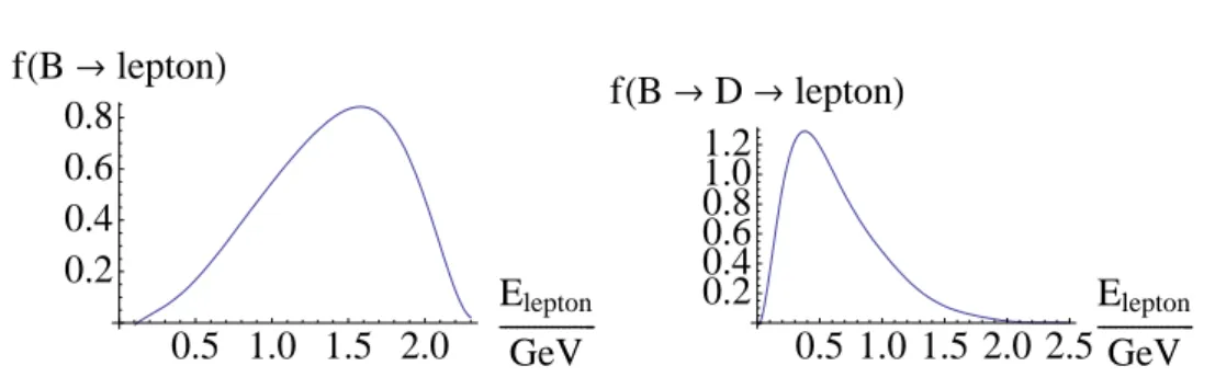
For instance, no collinear emission off a heavy quark is allowed due to its mass, in contrast to massless final state particles, where non-perturbative parton-to-hadron fragmentation functions or elaborated jet definitions have to be introduced to absorb divergences associated with particle splittings with zero angle. However, relating theory and experiment for heavy flavour production is not at all an easy task. Experiments usually detect heavy flavours by reconstructing heavy meson decays, e.g., semi-leptonic decay lepton spectra. To avoid unwanted bias from deconvoluting experimental results back to the heavy quark level, all theoretical calculations should be done as close as possible to the observational level. Therefore, we implement in our parton-level Monte Carlo codes also the hadronisation of the produced charm and bottom quarks into D and B mesons and their subsequent decays. Both can be modelled by additional non-perturbative functions extracted from experimental data [53–57].

In the spin-averaged case, next-to-leading order (NLO) calculations for single-inclusive heavy quark hadro- and photoproduction have been available for quite some time [58–

61], and partial results at the next-to-next-to-leading order level have been obtained recently [62–70]. In order to calculate also phenomenologically interesting heavy quark correlations, a parton-level Monte Carlo code, which integrates the phase space numer- ically, was developed in [71, 72]. Hadronisation into heavy mesons and their semilep- tonic decays were implemented later in [57]. In addition, our work allows the possibility of having longitudinally polarised initial states. This significantly extends previous, largely analytic calculations for spin-dependent heavy flavour production [73–76] which were limited to single-inclusive observables and could not include experimentally relevant acceptance cuts. We note that all order resummations of possibly large logarithms of the ratio of the transverse momentum and the mass of the heavy quark have been considered in the unpolarised case in references [77–82]. For the phenomenological applications in the polarised case studied in this work, resummation effects are expected to be small and hence ignored for the time being.

Another interesting observable related to heavy flavours is the so-called charge asymmetry which describes the difference of cross sections for producing a heavy quarkQor a heavy antiquark ¯Qat a certain point in phase space, respectively. This asymmetry probes a subset of NLO radiative corrections and vanishes in tree-level approximation.

It was studied in the context of top production in [83–85] in the unpolarised case. We study the corresponding polarised charge asymmetry [86, 87].

This thesis is organised as follows: In chapter 2 we start with briefly outlining the basic principles of QCD. We show how to derive the Feynman rules from the QCD Lagrangian and discuss the framework relevant for perturbative QCD calculations. We introduce the factorisation theorem, discuss the renormalisation procedure, and outline how to deal with collinear and infrared singularities at NLO accuracy. We review the current knowledge about unpolarised and longitudinally polarised parton density functions (PDFs) as well as the status of heavy quark production and hadronisation.

Chapter 3 is devoted to a detailed account of the theoretical framework. We discuss the ingredients of a perturbative QCD calculation at NLO accuracy. Special emphasis is put on the phase space integration where both largely analytical and numerical

(9)

methods are introduced. It is shown how experimentally relevant cross sections are obtained from the partonic hard scattering processes, which are presented in detail in chapter 4. Here, we also introduce the charge asymmetry.

In chapter 5 we present our phenomenological studies. We start with a comparison of the analytical and the numerical implementations of the phase space integration to validate our codes. Next, we present expectations for single-inclusive heavy quark distributions and the charge asymmetry for possible future experiments at GSI-FAIR and J-PARC. Then, we turn to hadroproduction at RHIC, where we give detailed results at the decay lepton level for both single-inclusive and correlation observables.

We study the sensitivity of the corresponding double spin asymmetries, defined as the ratio of polarised and unpolarised cross sections, to the polarised gluon distribution.

Currently available preliminary experimental results [18, 19, 88] are unfortunately not precise enough for a determination of ∆g(x).

We continue with presenting phenomenological results for photoproduction of charm and compare them to existing results from the COMPASS collaboration [20, 21, 51, 89].

We discuss a possible impact of our next-to-leading order results on the extraction of

∆g/g performed by COMPASS. We finish with expectations for photoproduction of charm and bottom quarks at a polarised lepton-proton collider currently considered and study the sensitivity of such measurements to the parton content of circularly polarised photons, which is completely unmeasured so far.

We summarise and conclude in chapter 6.

We note that some parts of this thesis, especially the phenomenological results in chapter 5, have already been published in peer-reviewed journals [87, 90, 91].

(10)

(11)

The basics of QCD 2

Quantum chromodynamics (QCD) describes the interaction caused by the strong force.

The particles subjected to it are quarks and gluons. Quarks are fermions of spin 1/2 and can be organised in different families. Three families have been experimentally detected up to now. It has been shown that the existence of more than three families has not been completely excluded; see, e.g., [12] for a review. However, the newest results show that this possibility is rather improbable [15, 16]. Each family contains up- and down-type quarks. Flavours belong to the fundamental representation and contain colour triplets.

The force between the quarks is mediated by gluons, the gauge particles of the strong interaction belonging to the adjoint representation. Gluons carry a colour charge and can interact with themselves due to non-Abelian parts in the Lagrange density.

Because of this non-Abelian structure, a closed solution of QCD has not been found yet, but several successful approximative methods have been developed.

In this chapter the basic ideas of QCD are introduced. As in many PhD theses, e.g., [52, 74, 92–94], we will only give a short account of the framework of QCD. Special emphasis is put on perturbative methods which will be used in the following chapters.

The literature treating this subject is very large. The interested reader is referred to more detailed textbooks; see, e.g, [95–98].

2.1 The Lagrangian of QCD

The Lagrange density

L_QCD=L_matter+L_{Y M}+L_gauge+L_ghost+Lθ¯ (2.1) contains all the rich phenomenology described by quantum chromodynamics. The first two terms are the classical part of the Lagrangian, which is invariant under local gauge transformations ofSU(3).

The “matter” part of QCD reads Lmatter =

nf

X

f=1

ψ¯f(iγ^µDµ−mf)ψf, (2.2)

where ψf is the Dirac field for a quark of massmf;γ^µ are the Dirac matrices, and

Dµ =∂µ−igsA^a_µT^a (2.3)

(12)

is the covariant derivative. The Einstein sum convention is implicitly understood for repeated indices. f is the summation index over the different flavours, which differ in their masses. The strong coupling is denoted byg_s, the vectorial gauge field for the gluons by A and the colour matrices by T. They satisfy the commutation relation defining the groupSU(3):

[Tâ, T^b] =ifâbcTc, (2.4) where fâbc, which is antisymmetric in its indices, is the structure constant of the group. The second term of the Lagrangian (2.1) is the Yang-Mills term. It describes the dynamics of the gluons and reads

LY M =−1

4F²=−1 4

8

X

a=1

F_µν^a F^µν,a. (2.5)

The last term of the field tensor

F_µνâ =∂_µAâ_ν−∂_νAâ_µ+g_sfâbcA^b_µA^c_ν (2.6) is necessary to assureSU(3) gauge invariance and accounts for the self-interaction of gluons in QCD.

The next step is to quantise the up to now classical Lagrangian. This is not unique and different methods exist for this purpose [99]. To this end, one adds gauge fixing and ghost terms [100] to the Lagrangian, which are for the transverse gauge

L_gauge=−1 2ξ

8

X

a=1

(∂_µA^µ,a)² (2.7)

and

L_ghost= (∂_µc¯_a)(δ^ac∂^µ−g_sf^acbA^µ,b)c_c. (2.8) Here ca is the scalar anti-commuting so-called Fadeev-Popov ghost field. Physical results do not depend on the details of gauge fixing. The ghost contribution, also called Fadeev-Popov term, assures unitarity and cancels effects by nonphysical polarisations of the gluons.

By fixing the gauge, one explicitly breaks the gauge symmetry of the Lagrangian. As a residual symmetry, the BRST symmetry remains.

We finally mention the term

Lθ¯= ¯θ g²

32π²F_µν^a F˜^aµν, (2.9)

where ˜Fâµν = ¹₂^µνλρF_λρâ with the Levi-Civita tensor ^µνλρ is the dual ofF_µνâ . This term arises from the topology of the vacuum. It does not affect perturbative calculations, because it can be written as the total derivative of a current, i.e., as a surface term in the action. It is important, however, for some non-perturbative observables.

For solving the QCD equations of motion, no completely analytical method has been found up to now due to its non-Abelian structure. Therefore, several approximative and numerical methods have been devised. The mostly used methods are Shifman- Vainshtein-Zakharov (SVZ) and light cone sum rules, the large NC limit, chiral perturbation theory, lattice QCD and perturbative QCD. Each of these methods has its advantages and shortcomings and is best suited for certain applications. The best approach for solving a certain problem in QCD depends on the nature of the problem.

(13)

2.1 The Lagrangian of QCD

As we focus in this thesis on scattering experiments characterised by large momentum transfers, we use the framework of perturbative QCD (pQCD). The presence of a hard scale keeps the expansion parameter, the coupling constantα_s,small, and, thus, allows for an expansion in α_s.One has noticed that α_s is not always small, but depends on the energy transfer of a regarded process. The observation that the coupling of QCD decreases at short distances is called asymptotic freedom.

The fact that QCD is a renormalisable quantum field theory has the consequence that gs has to be defined at a renormalisation scaleµr and varies with the 4-momentum transfer. Some details of renormalisation will be given in section 2.3 below. Nev- ertheless, we anticipate here the following important result of renormalisation: The scale evolution of the couplingαs(µ)≡^g²^s_4π^(µ) is predicted by the renormalisation group equation (RGE)

µdgs(µ)

dµ =β[gs(µ)] (2.10)

where the QCD beta function can be written as a power series β(gs) =−gs

∞

X

n=1

αs

4π n

βn. (2.11)

The first two terms have the form β1= 1

3(11NC−2nf) (2.12)

and

β2=1

3(102Nc−38nf) (2.13)

withN_c andn_f being the number of colours and flavours, respectively.

Up to NLO accuracy, one can use αs(µ) = 4π

β₁ln(µ²/Λ²)

1− β2

β²₁

ln[ln(µ²/Λ²)]

ln(µ²/Λ²)

(2.14) as an approximation. The fundamental parameter of QCD, Λ,has to be determined from experiment and is of the orderO(200 MeV) for dimensional regularisation.

As a result, perturbative QCD can only be applied for hard scales µΛ.

If the distance between two quarks increases, the momentum transfer decreases and as a consequence the coupling constant αs(µ) = ^g²^s_4π^(µ) will increase as shown in figure 2.1. Confinement is a consequence of this property: it is not possible to separate two quarks. If one tries to do so, due to the increasing coupling at large distances, a new quark-antiquark pair will be created from the vacuum, which will immediately form new hadrons with the separated quarks.

In the case thatα_sis small, i.e., at high momentum transfers and short distances, one can express any physical observable, e.g., a cross section [∆]σin a power series inα_s with coefficients [∆]Ai,

[∆]σ=

∞

X

i=0

αⁱ_s[∆]Ai, (2.15)

which in practise is truncated after a certain order due to the complexity of higher order corrections. We use the notation with the square bracket and the Delta to denote

(14)

unpolarised and longitudinally polarised quantities in one equation: without the ∆ one gets the equation for the unpolarised and with the ∆ for the longitudinally polarised observables.

Though unproven, it is generally assumed that the coefficients of QCD perturbative series are divergent, but the series expansion is asymptotic: A series is called asymptotic, if

Γ−

N

X

n=0

αⁿ_sΓ⁽ⁿ⁾

≤CN+1α^N+1_s (2.16)

for all integersN.

Even if summed to all orders, a series P∞

n=0αⁿ_sΓ⁽ⁿ⁾ does not necessarily define Γ in the limitαs →0. However, the generally good agreement of experimental results and theoretical calculations in the framework of perturbative QCD give evidence that pQCD is a helpful tool to describe experimental phenomena.

The qualitative behaviour of observables can often be estimated by leading order calculations. For precise, quantitative calculations, one has to account for higher order corrections, which are sizable. Theoretical calculations depend on unphysical scales if the series is cut off.

Therefore, consider a quantity Γ independent of the scaleµ:

0 =µ ∂

∂µΓ =µ ∂

∂µ

∞

X

n=0

αⁿ_sΓ⁽ⁿ⁾. (2.17)

If the perturbative series is truncated at order N, a scale dependence of the order α^N+1_s remains:

µ ∂

∂µ

N

X

n=0

αⁿ_sΓ⁽ⁿ⁾=−µ ∂

∂µ

∞

X

n=N+1

αⁿ_sΓ⁽ⁿ⁾. (2.18)

Generally, a reduction of the scale dependence and hence of the theoretical uncertainties is expected, when higher orders are included in the calculation.

2.2 Outline of the derivation of the Feynman rules

The starting point for the derivation of the so-called Feynman rules used in pQCD calculations is the action

SQCD=i Z

d⁴xLQCD. (2.19)

We want to calculate transitions from an initial state|iito a final state|fi.They are mediated by the operator

T{exp[−iS_int]},

where S_int is the interaction part of S_QCD. In the interaction picture, this operator can be expanded in a series in terms of the coupling and the resulting terms can be decomposed using Wick’s theorem. The results can be represented by Feynman diagrams.

The graphical representation of the Feynman diagrams is only a symbolic notation.

Each line and each vertex in a Feynman diagram can be translated into a mathematical

(15)

2.3 Divergences and renormalisation

QCD α (Μ ) = 0.1184 ± 0.0007s Z

0.1 0.2 0.3 0.4 0.5

α

_s

(Q)

1 10 100

Q [GeV]

Heavy Quarkonia e⁺e^–Annihilation

Deep Inelastic Scattering

July 2009

Figure 2.1: The running of the strong coupling constant. Taken from [101].

expression, as given in appendix A. The npoint functions can be used to determine Feynman rules. An n point function is the vacuum expectation value of the product ofnfield operators. The contributions from thesenpoint functions are after the Wick contraction sums and products of the propagators and vertex functions represented by Feynman rules.

2.3 Divergences and renormalisation

Calculations at the lowest order of the perturbative series, the tree level, are free of divergences, and relatively easy to perform, but in general not suitable for quantitative analyses. However, at higher orders, several types of divergences can be found:

ultraviolet ones, infrared or soft ones, and collinear ones.

First, one encounters divergences for loop graphs, which come from the behaviour of the integrals at large internal momenta. They are called ultraviolet (UV) divergences and can be eliminated by adding appropriate counterterms to the Lagrangian. A strong motivation for such a renormalisation is that the standard model can only be valid up to the Planck scale because there gravity gets important. At present there is no generally accepted method for the unification of the standard model and gravity. By redefining in an appropriate way the normalisation of the parameters of the Lagrangian, i.e., the mass and the coupling constants, the ultraviolet divergences can systematically be absorbed in each order of perturbation theory. This procedure is called renormalisation. ’t Hooft and Veltman have shown that QCD is a renormalisable quantum field theory [102].

(16)

From the behaviour of the loop integrals at low energies as well as from the phase space integration of particle momenta in the final state, infrared divergences can appear. Due to the Kinoshita-Lee-Nauenberg and the Bloch-Nordsieck [103] theorem, they cancel in the sum of all contributions up to the considered order. Collinear singularities are discussed below in detail and can be absorbed by the so-called mass factorisation.

In practise, the first step is to isolate the divergences or to make them manifest in a well- defined mathematical procedure. Different methods for this so-called regularisation exist. The most commonly adopted one is dimensional regularisation [102]. In this method, the number of the dimensions of space-time is – withε >0 – changed to 4+2ε for the infrared divergences and to 4−2εfor the ultraviolet ones. All these singularities manifest themselves as poles in 1/ε^pwithp∈ {1,2}in a NLO calculation. Although, in principle, one has to distinguish the ultraviolet and the infrared case, in practise, it is not explicitly necessary. It is sufficient to assumeε6= 0. After renormalisation and factorisation discussed in section 2.4, all 1/ε^p poles cancel. This property provides a valuable check for the correctness of practical calculations. A further great advantage of dimensional regularisation is that it respects the invariance of the theory under translation, boosts, and gauge transformations.

Let us now take a detailed look at the renormalisation of the Lagrange density. To work directly with the renormalised quantities, one employs a method to replace the existing bare parameters of the theory by their renormalised equivalents. This results in re-writing the Lagrangian as a part containing the renormalised parameters and a part containing the counterterms:

LQCD =L^R_QCD+Lcounterterms (2.20) with

Lcounterterms= (Z2−1)ψ_Ri /∂ψR−(Z2Zm−1)mRψ_RψR

+1

2(Z3−1)Aâ_µRδâb[g^µν∂^λ∂λ−∂^µ∂^ν]A^b_νR−( ˜Z3−1)câ_Rδâb∂^λ∂λc^b_R

−(Z1F −1)gsRψ_Rγ^µT^aψRA^a_µR−(Z1−1)1

2gsRfâbc(∂µAâ_νR−∂νAâ_µR)A^bµ_RA^cν_R

−(Z4−1)1

4g_sR² fâbcfâdeA^b_µRA^c_νRA^dµ_RAêν_R + ( ˜Z1−1)gsRfâbccâ_R∂µ(A^bµ_Rc^c_R). (2.21) The subscript R denotes the renormalised quantities. The Z are the multiplicative constants chosen to compensate the divergences. They obey

ψ=p

Z2ψR, A^µ=p

Z3A^µ_R, c= q

Z˜3cR, gs=ZggsR, ξ=Z₃ξ_R, m=Z_mm_R, Z₁=Z_gZ₃^3/2, Z_1F =Z_gZ₂Z₃^1/2,

Z˜₁=Z_gZ˜₃Z₃^1/2, Z₄=Z_g²Z₃². (2.22) From the conservation of the gauge invariance, one can derive the Slavnov-Taylor identities

Z1

Z3

= Z˜1

Z˜3

= Z1F

Z2

= Z4

Z1

. (2.23)

Apart from the divergences the renormalisation constants Zi can contain arbitrary finite pieces; the actual choice determines the renormalisation scheme. The most common one for QCD is the MS scheme [104], in which the 1/ε poles are subtracted

(17)

2.4 Factorisation theorem

along with certain finite terms which are characteristic for dimensional regularisation.

In practise, the renormalised Lagrange density leads to additional Feynman rules.

Adopting them, the UV singularities cancel.

Experimentally, neither free quarks nor free gluons have ever been observed. This phenomenon is called confinement. As the Lagrange density contains only quarks and not hadrons, one has to account for the complications originating from confinement. Due to the factorisation theorem discussed in the next section, the calculation of matrix elements can be split in pQCD in a non-perturbative part describing the long-range interactions, the parton distribution and fragmentation functions, and the perturbatively calculable cross sections on the partonic level. Another class of divergences appears in processes with identified hadrons: collinear singularities result, when the momentum of an emitted particle on an external line becomes parallel to the particle that emitted it. This leads to a diverging propagator. Note that collinear singularities have already been introduced and discussed in detail in [74, 86]. In the next section we will show how a redefinition of the non-perturbative functions can describe this phenomenon.

2.4 Factorisation theorem

We will start with setting the notation for the considered process:

H₁(K₁) +H₂(K₂)→h₁(P₁) +h₂(P₂) +X. (2.24) K1, K2andP1, P2denote here the four-momenta of the incoming and outgoing hadrons, respectively. As the subject of this work is heavy quark production, we can assume the h_i to be heavy quarks, as shown in figure 2.2, or mesons built from them. X contains all particles which are not observed. The reaction, as given in (2.24), corresponds to hadroproduction. In case of photoproduction, one has an incoming lepton or photon instead of one of the incoming hadrons H₁ or H₂. The factorisation theorem states that the hadronic cross section can be obtained through a convolution of the partonic cross sections calculated in perturbative QCD and the non-perturbative parton density functions [105–113]

d[∆]σ(µf) = [∆]f_a⁽¹⁾⊗[∆]f_b⁽²⁾⊗d[∆]σab(µf) +O Λ

pT

ⁿ

. (2.25)

In this equation the fragmentation functions of the heavy quarks are not included as they are fundamentally different from the ones of light (massless) quarks. The upper index corresponds to the number of the hadron or lepton or photon. The lower index denotes the parton in the parton density functionsf and the initially unrenormalised partonic cross section d[∆]σ_ab.Recall that the notation with the square bracket gives both the unpolarised (without the ∆) and the longitudinally polarised cross sections (with the ∆) in the same equation.

Here, using the symbols + and −for the two helicities and respecting parity conservation of QCD, dσ⁺⁺ =dσ⁻⁻ anddσ⁺⁻=dσ⁻⁺,the unpolarised and longitudinally polarised cross section can be defined by

dσ= 1

2[dσ⁺⁺+dσ⁺⁻] (2.26)

(18)

Figure 2.2: Cartoon illustrating factorisation for a generic single inclusive hadroproduction process. For simplicity, the notation is given here for the unpolarised case. The fragmentation functions of the heavy quarks are not shown as they are fundamentally different from the ones of light (massless) quarks.

and

d∆σ=1

2[dσ⁺⁺−dσ⁺⁻], (2.27)

respectively. Analogous definitions hold for the partonic cross sections, which will be denoted by d[∆]ˆσ. Defining f₊⁺ and f₊⁻ as the probability to find a parton with helicity + and−,respectively, in a hadron with helicity +,one definesf =f₊⁺+f₊⁻ and ∆f = f₊⁺−f₊⁻. In the notation adopted here, the +[−] sign denotes positive [negative] helicity.

The factorisation theorem is not exactly valid, but only up to so-called power correc- tionsO

Λ p_T

n

,which are not discussed further in this work as we consider high p_T processes.

In equation (2.25), the fragmentation (hadronisation) of the heavy quarks into mesons containing a heavy quark is not included because for heavy quarks in the final state, no collinear divergences arise due to their non-vanishing masses and therefore the cross sections with the heavy quark in the final state are finite – contrary to the light particle case. For the light particle case several sets of fragmentation functions have been determined by various groups [114–116]. They serve as an important ingredient in the extraction of polarised parton distribution functions which will be introduced below. In the heavy quark case, for a comparison with experimental observations, it is crucial to include a model for the fragmentation to heavy quark mesons and their subsequent decay. As this procedure is somewhat non-trivial, a detailed discussion of this problem will be given later in section 2.8.

The hadronic cross section has been separated into long and short range parts: The processes which take place at large length scales, i.e., at small momentum transfers, are described by the parton density functions discussed in the next section. The processes proceeding at small length scales, i.e, at large momentum transfers, can be calculated in perturbative QCD.

As it is not possible to control which partons with which momenta from the initial hadrons participate at the partonic process, one has to sum over all possible partons

(19)

2.4 Factorisation theorem

and to integrate over all kinematically allowed momentum fractions:

d[∆]σ(K₁, K₂) = X

i,j

Z 1 0

dy₁ Z 1

0

dy₂[∆]f_i⁽¹⁾(y₁, µ²_f)[∆]f_j⁽²⁾(y₂, µ²_f)d[∆]σ_ij(µ²_f, µ²_r, y₁K₁, y₂K₂). (2.28)

Recall that collinear divergences occur, when in a Feynman diagram the momentum of an internal particle gets parallel to an external massless one, because, in this case, the propagator of this internal particle is (quasi) on the mass shell and its denominator diverges. These divergences can be shifted by a redefinition of the bare parton densities into dressed ones, as will be described in detail in the following.

In the modified minimal subtraction (MS) scheme [104] used in this work the term γE−ln(4π),which always occurs in dimensional regularisation, is subtracted together with theεpoles.

Using the splitting functions [∆]P_ij(z),we define [∆]G_ij(z, µ²_f, µ²_r) = αs(µ²_r)

2π [∆]P_ij(z)

"

−1

ε+γE−ln(4π) + lnµ²_f µ²_r

#

. (2.29) The splitting functions [∆]P_ij(z) contribute here up toO(ε⁰),i.e., without theεparts.

For completeness, the [∆]P_ij(z) are listed in appendix B. Introducing

[∆]Γ_ij(z, µ²_f, µ²_r) =δ_ijδ(1−z) + [∆]G_ij(z, µ²_f, µ²_r), (2.30) the renormalised parton density functions are given by

[∆]f_l(xk, µ²_f) =X

i

Z 1 0

dyk

Z 1 0

dzkδ(xk−ykzk)[∆]f_i(yk, µ²_f)[∆]Γ_li(zk, µ²_f, µ²_r). (2.31) Using

d[∆]ˆσ⁽⁰⁾_ij =d[∆]σ⁽⁰⁾_ij (2.32) and

d[∆]ˆσ⁽¹⁾_ij (µ²_f, µ²_r) =d[∆]σ⁽¹⁾_ij (µ²_r)−d[∆]σ⁽¹⁾_M,ij(µ²_f, µ²_r), (2.33) where

d[∆]σ_M,ij=X

l,m

Z 1 0

dz1

Z 1 0

dz2[[∆]G_li(z1, µ²_f, µ²_r)δmjδ(1−z2)+

[∆]G_mj(z₂, µ²_f, µ²_r)δ_liδ(1−z₁)]d[∆]σ⁽⁰⁾_lm(z₁k₁, z₂k₂), (2.34) the result for the cross section is:

d[∆]σ(µ²_f, µ²_r) =X

a,b

[∆]f⁽¹⁾_a (µ²_f)⊗[∆]f⁽²⁾_b (µ²_f)⊗d[∆]ˆσ(µ²_f, µ²_r) (2.35) or more explicitly written

[∆]σ(K₁, K₂) = X

a,b

Z 1 0

dx1

Z 1 0

dx2[∆]f⁽¹⁾_a (x1, µ²_f)[∆]f_b⁽²⁾(x2, µ²_f)[∆]ˆσ_ab(µ²_f, µ²_r, x1K1, x2K2). (2.36) The symbol⊗is used as a shortcut to note a convolution. The [∆]ˆσabare finite.

(20)

2.5 The parton model and parton distribution functions

Deep-inelastic scattering has provided evidence for the existence of point-like constituents inside hadrons. These constituents are called partons. The term partons comprises both quarks and gluons.

The naive parton model was proposed before the advent of QCD. A fast moving hadron can be thought of as consisting of many collinear point-like constituents, the partons.

Later on, the separation of short- and long-distance physics as encoded in the factorisation theorem discussed above has provided the theoretical foundation of the parton model. In pQCD one can calculate partonic hard-scattering cross sections. However, only their hadronic counterparts are experimentally observable. The parton model and the factorisation theorem in particular relate them as stated, e.g., in equation (2.36).

The hadronic cross section can be expressed as a convolution of the non-perturbative parton distribution functions for each hadron with the calculable scattering cross sec- tionsd[∆]ˆσij of the two partonsiandj, as explained in the previous section.

As a consequence of the factorisation theorem, the parton densities fi(x, µ²_f), which describe physics at long distances, are universal, i.e., can be applied in calculations of different hadronic scattering cross sections.

The partonic cross sections that describe the physics at short distances, shall be calculated perturbatively. The scale, at which the separation of short- and long-distance phenomena is done, is set by the factorisation scale µf. The actual choice of µf is arbitrary and physical cross sections should not depend onµf.This leads to a powerful set of renormalisation group equations.

Perturbative QCD does not permit us to calculate size and form of the parton density functions, but their scale evolution is predicted by the DGLAP renormalisation group equations [117–119]. Hence, if one knows the parton density functions at one scale µ0, they can be predicted at any arbitrary scaleµ > µ0 with the help of the DGLAP equations.

In the lowest order, they read d[∆]g(x, µ²)

dlnµ² = αs(µ²) 2π

Z 1 x

dy y

"

X

q

[∆]Pgq(x/y)[∆]q(y, µ²) + [∆]Pgg(x/y)[∆]g(y, µ²)

#

(2.37) for the gluons and

d[∆]q(x, µ²)

dlnµ² =αs(µ²) 2π

Z 1 x

dy

y [[∆]Pqq(x/y)[∆]q(y, µ²) + [∆]Pqg(x/y)[∆]g(y, µ²)]

(2.38) for each quark flavour. It is also possible to write these coupled equations in compact matrix form. In the evolution of the quark parton density functions, the first term on the right hand side of equation (2.38) describes the possibility that a quark carrying a momentum fractionxcan have been produced by a quark with a larger momentum fraction y having emitted a gluon. Likewise, the second term results from the alter- native that a quark with momentum fraction x is produced by a gluon with larger momentum fraction. An analogous interpretation is valid for (2.37), which describes the possibilities to generate a gluon from a quark or a gluon.

The functions [∆]Pab(z) are the so-called splitting functions which are calculable in perturbative QCD [117, 120, 121]. They are listed in appendix B. In the case of

(21)

2.5 The parton model and parton distribution functions

x

10-4 10^-3 10^-2 10^-1 1

)2 xf(x,Q

0 0.2 0.4 0.6 0.8 1 1.2

g/10

d

d u

s u s, c c,

= 10 GeV2

Q2

x

10-4 10^-3 10^-2 10^-1 1

)2 xf(x,Q

0 0.2 0.4 0.6 0.8 1 1.2

x

10-4 10^-3 10^-2 10^-1 1

)2 xf(x,Q

0 0.2 0.4 0.6 0.8 1 1.2

g/10

d

d u

u s s, c c, b b,

GeV2

= 104

Q2

x

10-4 10^-3 10^-2 10^-1 1

)2 xf(x,Q

0 0.2 0.4 0.6 0.8 1 1.2

MSTW 2008 NLO PDFs (68% C.L.)

Figure 2.3: The unpolarised parton distributions of MSTW and their uncertainties. Figure taken from [128].

infrared corrections being absent, [∆]Pab(z) gives the probability to produce a parton of typeain a collinear splitting of a parton of typebwith a fractionzof its longitudinal momentum.

Taking into account also the helicity degree of freedom, unpolarised parton density functions are defined as the sum of the momentum distributions with parallel and antiparallel helicity of the hadron and parton, f₊⁺ andf₋⁺,respectively. The polarised ones, ∆f(x, µ²),are the difference between these two contributions, see equation (1.4).

Parton distribution functions need to be extracted from experiment. A functional form with several fit parameters is assumed. Using all relevant data, where factorisation applies and the partonic cross sections calculated in pQCD, a global fit can be performed.

In the unpolarised case, the most recent global fits have been done by the CTEQ and MSTW (former MRST) collaborations [122–127]. The results of the MSTW group are presented in figure 2.3. In the naive parton model, each valence quark carries one third of the total momentum of the proton. In the improved parton model, where it is not anymore assumed that each constituent quark has the same momentum and sea quarks come into play, one can nevertheless identify a peak in the u and d quark distributions around 1/3. The figure shows also the current uncertainty bands. In general, the uncertainty for the gluon distribution is larger than for the valence quarks.

Especially, in the limit x →1 the uncertainties grow for all parton distributions. It is a goal of further experiments, e.g., at the LHC, to pin down parton densities more precisely.

In leading order, the helicity dependent parton distribution functions are subject to the positivity constraint

|∆f(x, µ)|< f(x, µ).

Because the interpretation as a probability density is valid only at leading order, this

(22)

positivity constraint is – strictly speaking – not correct anymore at NLO. However, if the NLO corrections are not too large, it can be kept as an approximate constraint.

Positivity applies of course to physical cross sections, i.e.,|d∆σ| ≤dσ.

Earlier determinations of helicity dependent parton distribution functions only included DIS data and assumed a flavour symmetric sea [129]. The helicity dependent gluon distribution ∆g(x) was widely unconstrained, as in DIS processes the gluon does not enter at leading order.

A more recent work (DNS [130]) included semi-inclusive DIS data and resulted in two different sets of parton distribution functions related to different assumptions about fragmentation functions (Kretzer and KKP), which served as an additional non-perturbative input in the semi-inclusive DIS.

The state of the art is a first global fit including DIS, semi-inclusive DIS, and RHIC data [30, 31]. In particular, single-inclusive pion [131] and jet production [132], measured in spin-dependent proton-proton collisions at BNL-RHIC, have started to put significant limits on the amount of gluon polarisation in the nucleon [30]. New, preliminary single and di-jet data from the STAR collaboration [45] show for the first time tantalising hints for a non-zero ∆g(x, µ) [46, 133]. Due to the given kinematics, the current probes mainly constrain ∆g in the medium-to-largexregion, 0.05.x.0.2, which is not sufficient to determine its integral (the first moment) reliably.

It results in a rather small ∆gin the range of momentum fractions 0.05≤x≤0.2 as shown in figure 2.4. This region is mainly constrained by the RHIC data. Beyond this region, ∆g is still largely unconstrained. Therefore, the first moment ∆G, defined in equation (1.3), has still large uncertainties. Also improvements for the sea distributions have been achieved. Especially, a node in the ∆sdistribution and ∆¯u >0 and ∆ ¯d <0 have been found. In figure 2.4 the DSSV results and their error estimates are compared to older sets of parton distribution functions. Recall that all of them, except the DNS2005 sets, have a flavour symmetric sea. Note that from the asymmetry analysis collaboration the AAC03 parton density functions [134] are shown, as these ones will be used in chapter 5. The quark and antiquark distributions of the AAC08 analysis [135] are similar to AAC03. The AAC08 analysis provides two different sets, which, however, are very similar, except for the polarised gluon. One set has a gluon similar to AAC03, the other one – as DSSV – a gluon with a node. However, the absolute values of the AAC08 gluon are much larger than the DSSV gluon. For completeness, we note that also the PDFs of LSS2010 [136] show a moderate gluon, which is within the errors compatible with the analyses of DSSV and DSSV++ [46].

Some experiments have done their own analysis on ∆g/g. In this thesis, we will not discuss the methods used there. We only show the results in comparison to the DSSV values in figure 2.5. Most of the data points agree in the range of the errors with the DSSV fit.

We want to mention that another possible approach is that momenta of the parton density functions can be calculated on the lattice. But, only some low integer momenta are accessible on the lattice at the moment [138]. ∆g cannot be calculated in lattice QCD.

2.6 Photonic parton density functions

We will not only discuss heavy quark production in hadron-hadron scattering, but also in lepton-hadron scattering. The latter is measured by COMPASS at CERN and

(23)

2.6 Photonic parton density functions

0 0.1 0.2 0.3 0.4

-0.15 -0.1 -0.05 0 0.05

-0.04 -0.02 0 0.02

10^-2 10^-1

x( ∆ u + ∆ u

^–

)

DNS(KRE) DNS(KKP)

GRSV(std)

x( ∆ d + ∆ d

^–

)

DSSV AAC03

x∆u

^–

x∆d

^– ^GRSV(min)GRSV(max)

x∆s

^–

x

∆χ²=1 (Lagr. multiplier)

∆χ²=1 (Hessian)

x ∆ g

x Q

²

= 10 GeV

²

-0.2 -0.1 0 0.1 0.2 0.3

10^-2 10^-1

Figure 2.4: The polarised parton distributions from DSSV. The uncertainties are shown as resulting from two different methods applied by the DSSV group: the Lagrange multiplier and the Hessian method. More details about these two methods can be found in [31]. This figure has been adopted from a similar figure in [31].

Not shown are the very new DSSV++ [46] parton distribution functions. The function ∆g(x) from DSSV++ lies between the functions ∆g(x) from GRSV(std) and DSSV.

will be pursued in the future at an EIC. In this work, we are mainly concerned with photoproduction, where the photon is quasi-real. Its energy spectrum, i.e., the photons radiated off the lepton, can be described by the Weizs¨acker-Williams approximation.

This spectrum can be calculated in the framework of quantum electrodynamics (QED).

The results for the unpolarised and polarised cases are [139–143]

Pγl=αem

2π

1 + (1−y)²

y lnQ²_max(1−y)

m²_ly² + 2m²_ly 1

Q²_max −1−y m²_ly

(2.39) and

∆Pγl= αem

2π

1−(1−y)²

y lnQ²_max(1−y)

m²_ly² + 2m²_ly² 1

Q²_max −1−y m²_ly²

, (2.40)

(24)

COMPASS 2-had, Q²>1 GeV² COMPASS 2-had, Q²<1 GeV² COMPASS charm (prel) HERMES

SMC

DSSV Q²=1 GeV² DSSV Q²=10 GeV²

x

∆ g/g

-0.5 0 0.5

10^-1

Figure 2.5: Current experimental results on ∆g(x)/g(x).Some data points are taken from [22, 137].

respectively. The second terms in the square brackets give sizable contributions to the splitting functions for muons due to their large mass. These terms give important contributions to the calculations for COMPASS which has a muon beam.

In heavy quark production, the photon can interact with the hadron either directly by photon-gluon fusion or photon-(anti)quark-scattering in order to produce a heavy quark pair or fluctuate into quarks and gluons which enter the hard scattering process.

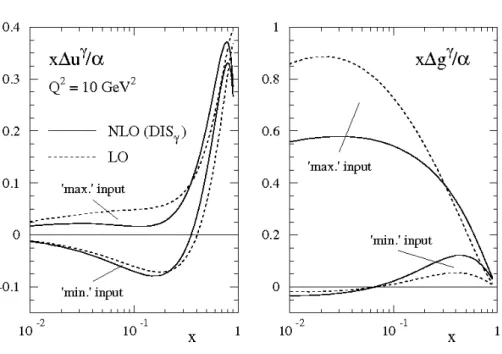
In the first case, one has [∆]fγ(x, µ) =δ(1−x). In the second – the resolved – one, the photon parton density functions have to be determined experimentally. In the unpolarised case most of the information on the non-perturbative hadronic structure of photons comes from γ^∗γ DIS in e⁺e⁻ annihilations. These unpolarised photon distribution functions are known as the GRVγ distributions [144]. As the circularly polarised parton distributions of the photon are completely unknown, only minimum and maximum scenarios as shown in figure 2.6 can be given.

Also for the photon parton density functions, evolution equations similar to the DGLAP equations exist; however, an additional inhomogeneity arises, since the photon can act as its own parton:

d[∆]qγ(x, µ) dlnµ = αs

2π([∆]kq(x, µ) +{[∆]Pqq⊗[∆]qγ+ [∆]Pqg⊗[∆]gγ}), (2.41) d[∆]gγ(x, µ)

dlnµ = αs

2π([∆]k_g(x, µ) +{[∆]P_gq⊗([∆]q_γ+ [∆]¯q_γ) + [∆]P_gg⊗[∆]g_γ}).

(2.42) Recall that the symbol⊗denotes (as usual) a convolution.

As a consequence, the solution of these inhomogeneous evolution equations has a point- like part [∆]fγ, pl,which can be calculated perturbatively, and a hadronic contribution

(25)

2.6 Photonic parton density functions

Figure 2.6: The minimum and maximum scenario for the polarised photon parton distribution functions for both LO and NLO at a scale of 10 GeV². The left and right panel show the photon parton density functions for the up quark and the gluon, respectively. Figure taken from [145].

[∆]fγ, had which follows from the solution of the according homogeneous equations, see, e.g., [52, 94]. The interested reader is referred to the literature for details.

It follows from the fact that the photonic parton density functions have a point-like and a hadronic component that cross sections with an incoming photon are composed of two parts: the direct and the resolved part:

∆σ= ∆σ_dir+ ∆σ_res. (2.43)

Experimentally measurable is only the sum of the direct and the resolved part of the cross section, but neither the direct part ∆σdir nor the resolved part ∆σres alone.

Indeed, for certain experimental constellations like charm production at COMPASS, the resolved contribution turns out to be small compared to the direct part, see our results in chapter 5.

Convoluting the photon content of the lepton as given by the Weizs¨acker-Williams spectrum, [∆]Pγl(y),and the photon parton distributionfγ functions, one gets for the parton density functions in a lepton the master formula

[∆]f(x_l, µ_f) = Z 1

x_l

dy

y [∆]P_γl(y)[∆]f_γ

x_γ =x_l y, µ_f

, (2.44)

which is valid both for the direct and the resolved case. The [∆]fγ are of the order of 1/αs. This has the consequence that the direct and the resolved contributions enter at the same perturbative order.